Momentum distributions and short-range correlations in the deuteron and ³He with modern chiral potentials

Abstract

We study momentum distributions and short-range correlation probabilities in $A$=2 and $A$=3 systems. First, we show results with phenomenological and meson-theoretic two- and three-nucleon forces to verify consistency with previous similar studies. We then apply most recent high-quality chiral nucleon-nucleon potentials up to fifth order in the chiral expansion together with the leading chiral three-nucleon force. Predictions are examined in the context of a broader discussion of short-range correlation probabilities extracted from analyses of inclusive electron scattering data, addressing the question of whether modern interactions can be reconciled with the latter.

I Introduction

The study of high-momentum distributions in nuclei is fundamentally important as it can reveal information about the short-range few-nucleon dynamics when the few-nucleon system under consideration is surrounded by the medium. In this work, we focus on short-range correlation (SRC) in the deuteron and, with particular emphasis, in ³He.

The lively discussion recently stimulated by inclusive electron scattering measurements at high momentum transfer on both light and heavy nuclei provides additional motivation for studying SRCs. In fact, those measurements have been analyzed with the purpose of extracting information on SRCs CLAS ; CLAS2 ; CLAS3 ; src ; Pia+ . In a suitable range of $Q^{2}$ (the four-momentum squared of the virtual photon) and of $x_{B}$ (the Bjorken variable), the cross section for the $A(e,e^{\prime})X$ process is factorized such that cross section ratios for nuclei $A_{1}$ and $A_{2}$ can be related to the respective probability of a nucleon to be involved in (either two-body or three-body) SRCs Egi06 . When extended to nuclear matter, this probability is equivalent to the “wound integral”, which measures the amount of correlations in the wave function and the $G$-matrix FS14 . We recall, in passing, that the wound integral is the integral of the amplitude squared of the “defect function”, defined as the difference between the correlated and the uncorrelated wave functions.

Information about two-body SRCs can also be obtained in coincidence experiments involving knock-out of a nucleon pair with protons Tang or electrons Korover ; Shneor ; Subedi ; Baghda .

The plateaus seen in the ratios of inclusive scattering cross section CLAS ; CLAS2 can be attributed to the dominance of SRCs for momenta above approximately 2 fm^-1. That is, when the electron scatters from a high-momentum nucleon in the nucleus, the scattering can be viewed as an electron-deuteron interaction, with the other $A-2$ nucleons essentially at rest. More specifically, in an appropriate range of $Q^{2}$ and $x_{B}$, the ratio

$$R(A_{1},A_{2})=\frac{\sigma(A_{1},Q^{2},x_{B})/A_{1}}{\sigma(A_{2},Q^{2},x_{B})/A_{2}}$$ (1)

is expected to display scaling behavior. Under those circumstances, the cross section ratio can be expressed as

$$\frac{\sigma(A_{1},Q^{2},x_{B})}{\sigma(A_{2},Q^{2},x_{B})}=\frac{A_{1}}{A_{2}}R(A_{1},A_{2})\;,$$ (2)

where $R$ is identified with the ratio of SRC probabilities in the two nuclei $A_{1}$ and $A_{2}$. Therefore, measurements of inclusive electron scattering cross section ratios in the appropriate kinematical region can be related to the ratio of SRC probabilities, and ultimately the absolute probability for a particular nucleus, given a suitable starting point, which, quite naturally, one would take to be the deuteron.

Deuteron momentum distributions in the context of SRCs were studied in Ref. src2015 using local and non-local realistic two-nucleon (2N) interactions. Those included: purely phenomenological local potentials, such as the Argonne $v_{18}$ av18 (AV18) or the Nijmegen II Nij models, non-local meson-theoretic models, such as the charge dependent Bonn (CDBonn) potential CD , and state-of-the-art non-local chiral potentials EM03 ; chinn5 ; ME11 . In the study of Ref. src2015 , it was concluded that predictions of high-momentum distributions in the deuteron with non-local meson-exchange forces or state-of-the-art chiral forces are systematically lower than those obtained with the local AV18 or Nijmegen II potentials. Note that the AV18 predictions were used in Refs. CLAS ; CLAS2 to extract empirical information for heavier nuclei based on Eqs. (1) and (2).

The analysis of Ref. src2015 highlights non-localities in the tensor force as the source of differences in SRC among the various predictions, and suggests that such model dependence should be taken into account, as it may impact SRC considerations for heavier nuclei, see comments just below Eq. (2). At this point, it is appropriate to recall that the presence of non-locality in the tensor force has been found since a long time to be a desirable feature in nuclear structure calculations. (For a discussion on the impact of non-locality in the one-pion exchange, see, for instance, Refs. MSS96 ; Polls98 ; MP99 .)

This paper contains updates and major extensions of the work of Ref. src2015 , presenting a simultaneous study of momentum distributions in the deuteron and in ³He. First, we calculate the deuteron momentum distribution using the most recent chiral 2N potentials from Ref. EMN , from leading to fifth chiral order. These interactions are better and more consistent than the ones of Refs. EM03 ; chinn5 ; ME11 used in Ref. src2015 , because the same power counting scheme and cutoff procedures are used at each order. In addition, the $\pi N$ low-energy constants (LECs) are the very accurate ones determined in the Roy-Steiner analysis of Ref. Hofe+ . The uncertainty associated with these LECs is sufficiently small that variations within their errors have negligible impact on the construction of the potentials, which are non-local and of soft nature. A point worth mentioning is that these 2N forces can predict a triton binding energy around 8.1 MeV, leaving only very small room for three-nucleon (3N) forces.

We then proceed to consider the single-nucleon (1N) and 2N momentum distributions in ³He using the phenomenological AV18 and the meson-theoretic CDBonn potentials, alone or augmented by 3N forces, namely the Urbana IX (UIX) model UIX in conjunction with AV18, and the Tucson-Merlbourne (TM) TM 3N force in conjunction with CDBonn. This will allow us to quantify the 3N force contributions within the framework of these older forces. To verify our calculations, results obtained with the AV18 and AV18/UIX potential models will be compared with the previous studies of Refs. Alv13 ; Alv16 ; Wir_web .

Having established a reliable baseline, we shift our focus to the more novel aspects of this work, namely the most recent high precision chiral 2N potentials EMN and corresponding chiral 3N force. The main motivation behind this calculation can be explained as follows. The presence of high-momentum components in the nuclear wave function is an indication of SRCs. At the two-body level, SRCs originate from the (repulsive) short-range central and tensor force, which, in the well-established and still popular meson-exchange phenomenology, are described by $\omega$- and $\rho$-meson exchange, respectively. Although realistic meson-theoretic or purely phenomenological interactions are frequently employed in contemporary calculations of nuclear structure and reactions, this approach has some intrinsic problems/limitations. First, the connection between the 2N and the applied 3N force does not rest on firm grounds. Second, no clear mechanism exists to quantify and control the theoretical uncertainty of a prediction. These problems are absent from the chiral effective field theory ($\chi$EFT) approach, which provides a well-defined prescription to develop nuclear forces in an internally consistent manner at each order of a systematic perturbative expansion. In fact, using effective degrees of freedom, namely hadrons (nucleons and pions), and maintaining a link with quantum chromodynamics (QCD) through the symmetries of low-energy QCD, $\chi$EFT has become a well-established and, in principle, model-independent framework to develop nuclear forces and quantify the theoretical uncertainty at each order of the expansion. Therefore, we find it both important and insightful to perform these calculations using state-of-the-art chiral interactions.

The paper is organized as follows: In Sec. II we set the stage with a brief discussion on the deuteron, while we address ³He in Sec. III. In the latter section, we will first present a brief review of the numerical techniques used to calculate the $A=3$ nuclear wave functions and the 1N and 2N momentum distributions. Then we will show and discuss results obtained with the older AV18 and CDBonn potential models, augmented or not by the UIX UIX and the TM TM 3N force, respectively, as well as the chiral 2N potentials of Ref. EMN , without or with the chiral 3N force. We will also discuss the procedure adopted to determine the two LECs entering the leading 3N force. Our conclusions and future plans are summarized in Sec. IV.

II High-momentum distribution and SRCs in the deuteron

Figure 1: Left panel: Momentum distributions in the deuteron predicted with the chiral potentials of Ref. EMN at LO (dotted), NLO (dash-double dot), N²LO (dash-dot), N³LO (dash), N⁴LO (solid). The cutoff is fixed at $\Lambda=500$ MeV. Right panel: Predictions taken from Ref. src2015 , and are obtained using the chiral potentials of Ref. EM03 ; chinn5 ; ME11 .

Table 1: Probabilities of SRCs as defined in Eq. (3) and deuteron $D$-state percentage for the chiral interactions considered on the left panel of Fig. 1. The values in parenthesis, given for comparison, are taken from Ref. src2015 and correspond to the distributions shown on the right panel of Fig. 1. The cutoff $\Lambda$ is equal to 500 MeV in all cases.

Model	$a_{2N}(d)$	$P_{D}$
LO	0.046 (0.047)	0.0729 (0.0757)
NLO	0.015 (0.015)	0.0340 (0.0313)
N2LO	0.026 (0.022)	0.0449 (0.0417)
N3LO	0.024 (0.030)	0.0415 (0.0451)
N4LO	0.024 (0.026)	0.0410 (0.0414)

To best put this study in context, we begin with a quick review of the 2N bound state. In particular, we present in Fig. 1 the deuteron momentum distributions $\rho(k)$, defined as the Fourier transform squared of the coordinate-space deuteron wave function. On the left side of the figure, we show the results, with focus on high-momentum components, obtained with the latest chiral interactions of Ref. EMN from leading to fifth order (N⁴LO). On the right side of the figure, we show for comparison the same quantities calculated as in Ref. src2015 with the older chiral potentials of Refs. EM03 ; chinn5 ; ME11 . From inspection of the figure, we can conclude that the convergence pattern has definitely improved with the new potentials.

We then define the probability of SRCs in the deuteron as in Ref. src2015 , i.e.

$$a_{2N}(d)=4\pi\int_{k^{-}}^{\infty}\rho(k)k^{2}\;dk\;,$$ (3)

where $k^{-}$ is taken to be 1.4 fm^-1 (276 MeV). This definition was adopted in Ref. CLAS , where the choice of the lower integration limit was suggested by the onset of scaling of the cross section, which should signal the dominance of scattering from a strongly correlated nucleon. In view of Eqs. (1)–(2), the absolute per-nucleon SRC probability in a nucleus $A$ can be deduced if the absolute per-nucleon probability in ³He and the deuteron are calculated or estimated. More precisely,

$$a_{2N}(A)=a_{2}(A/^{3}{\rm He})a_{2N}(^{3}{\rm He})\;\;\;\;\mbox{and}\;\;\;\;a_{2N}(^{3}{\rm He})=a_{2}(^{3}{\rm He}/d)a_{2N}(d)\;,$$ (4)

where $a_{2}(A_{1}/A_{2})$ is the SRC probability for nucleus $A_{1}$ relative to nucleus $A_{2}$. The probability in the deuteron was taken to be equal to $0.041\pm 0.008$ in Ref. CLAS2 . We list in Table 1 the integrated probabilities $a_{2N}(d)$ defined in Eq. (3), calculated integrating the curves of Fig. 1 (left panel). As an additional, related information, we also show the corresponding $D$-state percentage. In fact, deuteron $D$-state probabilities are larger with stronger short-range central and tensor components of the nuclear force which, for the non-local chiral interactions and, generally, for non-local interactions, are softer than for the local AV18 potential. The values in parenthesis correspond to the distributions displayed on the right of Fig. 1, i.e. obtained with the older chiral potentials of Refs. EM03 ; chinn5 ; ME11 . As the table shows, there are huge variations between the LO and the NLO cases, and still large differences between NLO and N²LO. Variations at higher orders indicate a clear convergence pattern, definitely improved by the use of the newest potentials. Finally we notice that the deuteron integrated probabilities $a_{2N}(d)$ display significant model-dependence, as the corresponding values obtained with the AV18 and the CDBonn potentials are 0.042 and 0.032, respectively. We will show below that similar considerations apply to ³He as well. This model dependence is likely to propagate in the analyses for heavier nuclei.

III High-momentum distribution and SRCs in the ³He nucleus

III.1 Theoretical formalism

We briefly review the method used to solve the $A=3$ quantum mechanical problem, i.e. the Hyperspherical Harmonics (HH) method. This method has the great advantage that we can work both in coordinate- and momentum-space, with no restriction on the choice of the nuclear potential model, either local or non-local. The starting point are the so-called Jacobi coordinates, which are defined in coordinate-space as Viv06 ; Kie08

$${\bf x}_{p} = \frac{1}{\sqrt{2}}({\bf{r}}_{j}-{\bf{r}}_{i})\ ,$$

$${\bf y}_{p} = \sqrt{\frac{2}{3}}\left({\bf{r}}_{k}-\frac{1}{2}({\bf{r}}_{i}+{\bf{r}}_{j})\right)\ ,$$ (5)

where $p$ represents an even permutation of $i,j,k=1,2,3$, with $p=1$ for $i,j,k=2,3,1$, and ${\bf r}_{i}$ is the position of the $i$-th particle. The conjugate Jacobi momenta (in unit of $\hbar=1$) are defined as

$${\bf q}_{p} = \frac{1}{\sqrt{2}}({\bf{p}}_{j}-{\bf{p}}_{i})\ ,$$

$${\bf k}_{p} = \sqrt{\frac{2}{3}}\left({\bf{p}}_{k}-\frac{1}{2}({\bf{p}}_{i}+{\bf{p}}_{j})\right)\ ,$$ (6)

${\bf{p}}_{i}$ being the momentum of the $i$-th particle. The next step is to introduce the so-called hyperradius $\rho$ and hypermomentum $Q$ as

$$\rho = \sqrt{{\bf x}_{p}^{2}+{\bf y}_{p}^{2}}\ ,$$

$$Q = \sqrt{{\bf k}_{p}^{2}+{\bf q}_{p}^{2}}\ ,$$ (7)

and the hyperangle $\phi_{p}^{(\rho/Q)}$, given by

$$\tan\phi_{p}^{(\rho)} = \frac{y_{p}}{x_{p}}\ ,$$

$$\tan\phi_{p}^{(Q)} = \frac{k_{p}}{q_{p}}\ .$$ (8)

We note that $\rho$ and $Q$ do not depend on the considered permutation, while $\phi_{p}^{(\rho)}$ or $\phi_{p}^{(Q)}$ do. Then, the HH functions for the $A=3$ system are given in coordinate space by

$${\cal Y}_{\alpha,n}(\Omega^{(\rho)}_{p})=[[Y_{l}({\hat{\bf x}}_{p})\otimes Y_{L}({\hat{\bf y}}_{p})]_{\Lambda\Lambda_{z}}\otimes[\chi_{S_{ij}}\otimes\frac{1}{2}]_{\Sigma\Sigma_{z}}]_{JJ_{z}}[\eta_{T_{ij}}\otimes\frac{1}{2}]_{TT_{z}}P_{n,l,L}(\phi_{p}^{(\rho)})\ ,$$ (9)

where $\Omega^{(\rho)}_{p}=(\phi_{p}^{(\rho)},{\hat{\bf x}}_{p},{\hat{\bf y}}_{p})$ and

$$P_{n,l,L}(\phi_{p}^{(\rho)})=N_{n,l,L}(\cos\phi_{p}^{(\rho)})^{l}(\sin\phi_{p}^{(\rho)})^{L}P_{n}^{L+1/2,l+1/2}(\cos 2\phi_{p}^{(\rho)})\ ,$$ (10)

$N_{n,l,L}$ being a normalization coefficient and $P_{n}^{L+1/2,l+1/2}(\cos 2\phi_{p}^{(\rho)})$ a Jacobi polynomial of degree $n$. In Eq. (9), $Y_{l}({\hat{\bf x}}_{p})$ and $Y_{L}({\hat{\bf y}}_{p})$ are spherical harmonics in the two Jacobi coordinates, coupled to the total orbital angular momentum $\Lambda,\Lambda_{z}$, $\chi_{S_{ij}}$ ($\eta_{T_{ij}}$) is the spin (isospin) function of the pair $ij$, where the spins (isospins) of the particles $i$ and $j$ are coupled to $S_{ij}$ ($T_{ij}$), which is itself coupled to the spin (isospin) 1/2 of particle $k$ to give the total spin (isospin) $\Sigma,\Sigma_{z}$ ($T,T_{z}$). The total orbital angular momentum $\Lambda$ and the total spin $\Sigma$ are coupled to the total angular momentum $J,J_{z}$. Finally, we remark that the grand-angular momentum is defined as $G=2n+l+L$, and we have labelled with the channel index $\alpha$ the set of quantum numbers $[l,L,\Lambda,S_{ij},\Sigma,T_{ij},T]$ which determine the spin-isospin-angular state. An expression similar to Eq. (9) holds in momentum-space, with appropriate changes.

Having introduced the HH functions, the $A=3$ nuclear wave function can be written as

$$\Psi=\sum_{\alpha,n}u_{\alpha,n}(\rho)\sum_{p}{\cal{Y}}_{\alpha,n}(\Omega_{p}^{(\rho)})\ ,$$ (11)

where $u_{\alpha,n}(\rho)$ is the hyperradial function to be determined. Similarly, in momentum-space we can write

$$\Psi=\sum_{\alpha,n}w_{\alpha,n}(Q)\sum_{p}{\cal{Y}}_{\alpha,n}(\Omega_{p}^{(Q)})\ ,$$ (12)

where $w_{\alpha,n}(Q)$ is the function of the hypermomentum $Q$, and it is related to $u_{\alpha,n}(\rho)$ via essentially a Fourier transform Viv06 , i.e.

$$w_{\alpha,n}(Q)=(-i)^{G}\int_{0}^{\infty}d\rho\,\frac{\rho^{5}}{{Q\rho}^{2}}\,{\cal J}_{G+2}(Q\rho)u_{\alpha,n}(\rho)\ ,$$ (13)

where ${\cal J}_{G+2}(Q\rho)$ is a Bessel function. Finally, the functions $u_{\alpha,n}(\rho)$ (or $w_{\alpha,n}(Q)$) are themselves expanded on a basis of Laguerre polynomials (or their Fourier transform) as

$$u_{\alpha,n}(\rho) = \sum_{k}c_{\alpha,n,k}\,\,\,^{(5)}L_{k}(\gamma\rho)\,{\rm e}^{-\gamma\rho/2}\ ,$$ (14)

where $c_{\alpha,n,k}$ are unknown coefficients and $\gamma$ is a non-linear parameter, chosen to be 4 fm^-1 for the local AV18 or AV18/UIX potentials, and 7 fm^-1 for the other non-local potentials. These values are the ones used in Refs. Viv06 ; Kie08 . Equations (11)–(14) can be cast in a compact form as

$$\Psi=\sum_{\mu}c_{\mu}\phi_{\mu}\ ,$$ (15)

where $\phi_{\mu}$ are given either in coordinate- or momentum-space. What is essential is that the $c_{\mu}$ coefficients of the expansion are the same in both cases. These coefficients are determined using the Rayleigh-Ritz variational principle, and the problem of determining $c_{\mu}$ and the energy $E$ is reduced to a generalized eigenvalue problem,

$$\sum_{\mu^{\prime}}c_{\mu^{\prime}}\langle\phi_{\mu}|H-E|\phi_{\mu^{\prime}}\rangle=0\ .$$ (16)

The advantage of having $\phi_{\mu}$ expressed either in coordinate- or in momentum-space is clear: the matrix elements of local operators will be calculated in coordinate-space, those of non-local operators in momentum-space. Furthermore, the 1N and 2N momentum-distributions can be written straightforward in momentum-space, without the need to perform any additional Fourier transform, unlike what was done in Refs. Alv13 ; Alv16 ; Wir_web . We will define and evaluate these momentum-distributions in the next sections.

We conclude this section by discussing the construction of the 3N force in the chiral approach. As is well known, the chiral 3N force appears for the first time at N2LO. It consists of three contributions: the two-pion exchange (2PE) term, the one-pion exchange (1PE) diagram, and a short-range contact term. The 1PE and the contact terms are multiplied by two LECs, $c_{D}$ and $c_{E}$, respectively. We determine them within a well established procedure (see Ref. Mar12 and references therein), repeated in Ref. nuclmatt18 for the new chiral potentials of Ref. EMN . In particular, the LECs $c_{D}$ and $c_{E}$ are constrained to reproduce the $A=3$ binding energies and the Gamow-Teller (GT) matrix element of tritium $\beta$-decay. For completeness, the values of $c_{D}$ and $c_{E}$ from Table I and II of Ref. nuclmatt18 are reported again here in Table 2 and 3, which include, in addition, the values obtained with $\Lambda=550$ MeV. In the first table, the $c_{D}$ and $c_{E}$ values are obtained using the 3N force up to N2LO. The complete 3N force beyond N2LO is very complex and often neglected in nuclear structure studies. However, the 2PE component of the 3N force can be calculated fully up to N4LO. In Ref. Kre12 it was shown that the 2PE 3N force has essentially the same analytical structure at N2LO, N3LO, and N4LO. Thus, one can add the three orders of this 3N force component and parametrize the result in terms of effective LECs. These effective LECs are taken from Table IX of Ref. EMN and shown here in Table 3. By using these $c_{1,3,4}$ in the mathematical expression of the N2LO 3N force, one can include the 2PE parts of the 3N force up to N3LO and N4LO in a simple way. Obviously, the LECs $c_{D}$ and $c_{E}$ are fitted again for each case and are listed in Table 3. The error arising from the fitting procedure, shown in parentheses, is quite large. On the other hand, we have observed that the impact of the 3N interaction on the momentum distributions and SRCs is weak (see below). Thus, we find it appropriate to use in our study the wave functions obtained adopting the central values of $c_{D}$ and $c_{E}$.

Table 2: Values for the LECs $c_{1,3,4}$, $c_{D}$ and $c_{E}$ at the chiral orders N2LO, N3LO and N4LO. The $c_{D}$ and $c_{E}$ LECs reproduce the $A=3$ binding energies and the GT matrix element in tritium $\beta$-decay, as explained in the text. The 2PE N3LO 3N interactions are not included, i.e. the $c_{1,3,4}$ LECs in the 3N force are those of Table II of Ref. EMN . The numbers in parentheses indicate the error arising from the fitting procedure.

	$\Lambda$ (MeV)	$c_{1}$	$c_{3}$	$c_{4}$	$c_{D}$	$c_{E}$
N2LO	450	–0.74	–3.61	2.44	0.935(0.215)	0.12(0.04)
	500	–0.74	–3.61	2.44	0.495(0.195)	–0.07(0.04)
	550	–0.74	–3.61	2.44	–0.140(0.190)	–0.44(0.03)
N3LO	450	–1.07	–5.32	3.56	0.675(0.205)	0.31(0.05)
	500	–1.07	–5.32	3.56	–0.945(0.215)	–0.68(0.04)
	550	–1.07	–5.32	3.56	–1.610(0.220)	–1.69(0.03)
N4LO	450	–1.10	–5.54	4.17	1.245(0.225)	0.28(0.05)
	500	–1.10	–5.54	4.17	–0.670(0.230)	–0.83(0.03)
	550	–1.10	–5.54	4.17	–1.245(0.175)	–1.91(0.02)

Table 3: Same as Table 2 but including the 2PE 3N interaction at N3LO and N4LO, i.e. the $c_{1,3,4}$ LECs in the 3N force are those of Table IX of Ref. EMN .

	$\Lambda$ (MeV)	$c_{1}$	$c_{3}$	$c_{4}$	$c_{D}$	$c_{E}$
N2LO	450	–0.74	–3.61	2.44	0.935(0.215)	0.12(0.04)
	500	–0.74	–3.61	2.44	0.495(0.195)	–0.07(0.04)
	550	–0.74	–3.61	2.44	–0.140(0.190)	–0.44(0.03)
N3LO	450	–1.20	–4.43	2.67	0.670(0.210)	0.41(0.05)
	500	–1.20	–4.43	2.67	–0.750(0.210)	–0.41(0.04)
	550	–1.20	–4.43	2.67	–1.350(0.200)	–1.14(0.03)
N4LO	450	–0.73	–3.38	1.69	0.560(0.220)	0.46(0.05)
	500	–0.73	–3.38	1.69	–0.745(0.225)	–0.15(0.04)
	550	–0.73	–3.38	1.69	–1.030(0.200)	–0.57(0.02)

III.2 Single-nucleon momentum distributions and corresponding integrated SRC probabilities

The 1N momentum distributions for a particular nucleon ($p$ or $n$) with momentum ${\bf k}$ in ³He are defined as

$$n^{p/n}(k)=\frac{1}{2}\int d{\hat{\bf k}}\;d{\bf q}\,\Psi^{\dagger}({\bf k},{\bf q})P_{p/n}\Psi({\bf k},{\bf q})\ ,$$ (17)

where we have fixed the permutation to be $p=1$, i.e. the particular nucleon is fixed to be particle $1$, and therefore ${\bf k}={\bf k}_{p=1}$ and ${\bf q}={\bf q}_{p=1}$, in the notation of Eq. (6). Furthermore, $P_{p/n}$ is the proton/neutron projection operator acting on particle 1. With this definition, the 1N momentum distributions are normalized as

$$4\pi\int k^{2}\,dk\,n^{n/p}(k)=1\ .$$ (18)

We have verified that Eqs. (17) and (18) are consistent with those of Ref. Alv13 .

We have first calculated the 1N momentum distributions using the AV18 av18 or CDBonn CD phenomenological potentials, with and without the 3N force (UIX UIX or TM TM for AV18 or CDBonn, respectively). The results are shown in Fig. 2. From those, we conclude that 3N force contributions are small, and only noticeable for $k\geq 2$ fm^-1. On the contrary, potential-model dependence is large in the range $k\geq 2$ fm^-1, an aspect which will be a recurrent theme throughout this paper. To avoid an excessively cumbersome presentation, we are not showing the results of Ref. Alv13 and Ref. Wir_web , obtained using AV18 HH and AV18/UIX Variational Monte Carlo (VMC) wave functions. However, we have verified that we are in agreement with Refs. Alv13 ; Wir_web , with small differences only in the high-$k$ tail of the distributions. Comparison between our results and those of Refs. Alv13 ; Alv16 ; Wir_web will be shown in the case of the back-to-back 2N momentum distribution (see below).

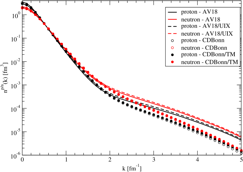
Figure 2: (Color online) The 1N momentum distributions $n^{p/n}(k)$, calculated using the AV18 and CDBonn 2N interaction, AV18/UIX and CDBonn/TM 2N and 3N interaction models.

We then move to study the 1N momentum distributions using chiral potentials EMN . In Figs. 3 and 4 we present the neutron and proton 1N momentum distribution obtained with only 2N forces at LO, NLO, N2LO, N3LO and N4LO on the left panel, and adding the 3N force, with LECs from Table 2 (model I) or 3 (model II). These 1N momentum distributions are calculated with cutoff value fixed at $\Lambda=500$ MeV. The figure shows that, for small values of $k$, all predictions at NLO and higher orders are quite similar. Overall, differences between the N3LO and N4LO curves are small enough to suggest a reasonable convergence pattern. The 3N force contributions are found again to be very small, and therefore the differences between the predictions from model I and model II for the 3N force are even smaller.

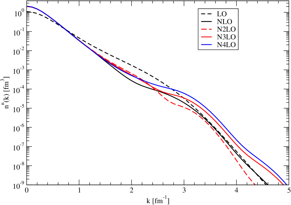
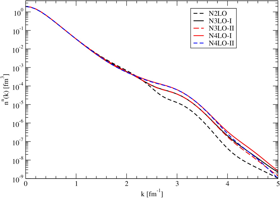
Figure 3: (Color online) The neutron momentum distributions $n^{n}(k)$, calculated using only 2N (left panel) and 2N+3N (right panel) chiral interactions, with $\Lambda=500$ MeV. The different chiral order are labelled as in the text. In particular, on the right panel, we have indicated with “I” and “II” the results obtained using the LECs of Table 2 and 3, respectively.

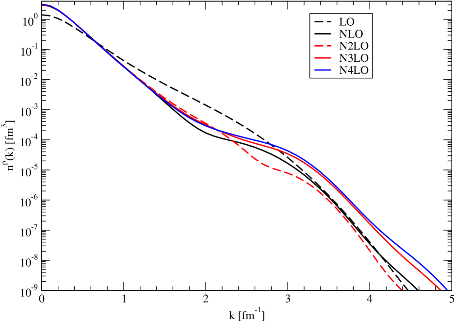
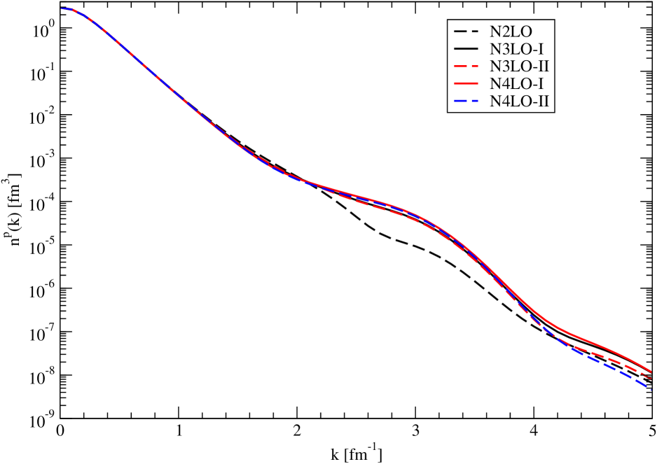
Figure 4: Same as Fig. 3 but for the proton momentum distributions $n^{p}(k)$.

The 1N momentum distributions $n^{n}(k)$ and $n^{p}(k)$ calculated with and without 3N interaction, at different chiral orders and for different values of the cutoff $\Lambda$, are shown in Figs. 5 and 6, respectively. By inspection of the figures, we can see that cutoff dependence appears comparable at all orders. Naturally, sensitivity is more pronounced in the high $k_{rel}$ region, where larger values of the cutoff produce “harder” distributions. Note, also, that cutoff-induced differences become noticeable where the distributions are reduced by about 5 or 6 orders of magnitude from their maximum values.

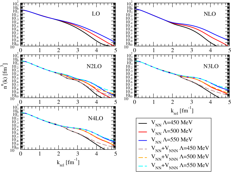
Figure 5: (Color online) The neutron momentum distributions $n^{n}(k)$, calculated using only 2N (solid lines) and 2N+3N (dashed lines) chiral interactions, at different chiral order and for three values of the cutoff $\Lambda=450,500,550$ MeV. The LECs of the 3N interaction are those of Table 3.

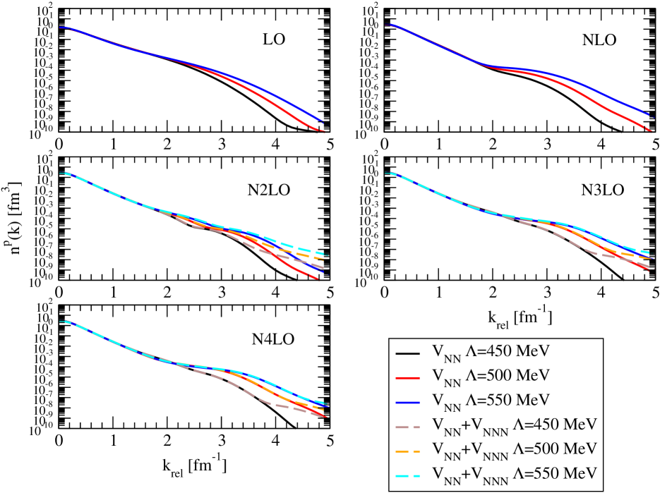
Figure 6: Same as Fig. 5 but for the proton momentum distributions $n^{p}(k)$.

Finally we consider the integrated probabilities, defined as

$${\cal{P}}^{p/n}(k^{-})=4\pi\int_{k^{-}}^{\infty}n^{p/n}(k)\,k^{2}\,dk$$ (19)

as in Table II of Ref. Alv13 . The results obtained with the 2N and 2N+3N phenomenological potentials are listed in Table 4. Those obtained using the chiral potentials are presented in Table 5. In both tables, we have first calculated ${\cal{P}}^{p/n}(k^{-}=0)$, in order to verify that the 1N momentum distributions are properly normalized. Note that in our integration, the upper limit of the integral is in fact 5 fm^-1. Therefore, the difference of ${\cal{P}}^{p/n}(k^{-}=0)$ from unity (see Eq. (18)) gives an indication of the importance of the tail of the momentum distribution. By inspection of the tables we can see that ${\cal{P}}^{p/n}(k^{-}=0)\simeq 1$ within 0.2–0.3%. A comparison of the results of Table 4 and 5 shows again a remarkable model dependence. The results of Table 5 show also a satisfactory order-by-order convergence.

Table 4: The integrated $p/n$ probabilities, as defined in Eq. (19), obtained with the various phenomenological potential models, i.e. AV18, CDBonn, AV18/UIX and CDBonn/TM, varying the integration lower bound $k^{-}$, given in fm^-1. We report also the values of Table II of Ref. Alv13 , obtained with the AV18 potential model.

	$P^{n}(k^{-})$		$P^{p}(k^{-})$
	$k^{-}=0.0$	$k^{-}=1.5$	$k^{-}=0.0$	$k^{-}=1.5$
AV18	0.997	0.068	0.997	0.041
AV18/UIX	0.997	0.077	0.998	0.048
CDBonn	0.998	0.052	0.998	0.031
CDBonn/TM	0.998	0.054	0.999	0.033
Ref. Alv13	0.999	0.067	1.000	0.041

Table 5: Same as Table 4 but obtained with chiral potentials, at different chiral orders, for different values of the cutoff $\Lambda$, 450, 500 and 550 MeV, also with the inclusion of the 3N force (lines labelled N2LO/N2LO at N2LO, N3LO/N3LO-I and N3LO/N3LO-II at N3LO, N4LO/N4LO-I and N4LO/N4LO-II at N4LO). The labels “I” and “II” refer to the LECs of Table 2 and 3, respectively.

	$P^{n}(k^{-}=0.0)$			$P^{p}(k^{-}=0.0)$			$P^{n}(k^{-}=1.5)$			$P^{p}(k^{-}=1.5)$
Model/$\Lambda$ [MeV]	450	500	550	450	500	550	450	500	550	450	500	550
LO	1.000	1.000	0.999	1.000	0.999	0.999	0.090	0.105	0.113	0.076	0.089	0.095
NLO	0.999	0.999	0.999	0.999	0.999	0.998	0.020	0.025	0.033	0.013	0.016	0.023
N2LO	0.999	0.999	0.999	0.999	0.999	0.999	0.033	0.040	0.046	0.020	0.024	0.027
N2LO/N2LO	0.999	0.999	0.999	0.999	0.999	0.999	0.033	0.040	0.046	0.020	0.024	0.027
N3LO	0.999	0.999	0.999	0.999	0.999	0.999	0.042	0.038	0.041	0.025	0.025	0.026
N3LO/N3LO-I	0.999	0.999	0.999	0.999	0.999	0.999	0.045	0.041	0.045	0.027	0.028	0.030
N3LO/N3LO-II	0.999	0.999	0.999	0.999	0.999	0.999	0.045	0.041	0.045	0.027	0.027	0.029
N4LO	0.999	0.999	0.999	0.999	0.999	0.999	0.041	0.039	0.043	0.024	0.025	0.026
N4LO/N4LO-I	0.999	0.999	0.999	0.999	0.999	0.999	0.043	0.043	0.048	0.026	0.028	0.030
N4LO/N4LO-II	0.999	0.999	0.999	0.999	0.999	0.999	0.043	0.042	0.046	0.026	0.027	0.028

A glance at Figs. 2 – 6, reveals characteristic differences between the qualitative features of the chiral predictions as compared to the phenomenological and meson-theoretic ones. This is due to the polynomial structure of the (short-range) contact terms used in the construction of the chiral potentials, combined with the exponential regulator function

$$f(p^{\prime},p)=\exp[-(p^{\prime}/\Lambda)^{2n}-(p/\Lambda)^{2n}]\;.$$ (20)

In the meson-theoretic potentials, the short range is described by heavy-meson exchanges represented by Yukawa functions of heavy-meson masses. On the other hand, the phenomenological AV18 potentials uses a Woods-Saxon function to provide the short-range core. (Heavy mesons, of course, have no place in chiral EFT.) Overall, the chiral predictions fall off at a faster rate as compared to the phenomenological ones. This is to be expected from the “softer” nature of the chiral potentials.

III.3 Two-nucleon momentum distributions and corresponding integrated SRC probabilities

The 2N momentum distribution of the $N_{1}N_{2}$ pair, with $N_{1}N_{2}=np$ or $pp$, as a function of their relative momentum $k_{rel}$, is defined as

$$n^{N_{1}N_{2}}(k_{rel},K_{c.m.})=\int d{\hat{\bf k}}_{rel}\int d{\hat{\bf k}}_{c.m.}\Psi^{\dagger}({\bf k}_{rel},{\bf K}_{c.m.})P_{N_{1}N_{2}}\Psi({\bf k}_{rel},{\bf K}_{c.m.})\ ,$$ (21)

where $P_{N_{1}N_{2}}$ is the projection operator on the $N_{1}N_{2}$ pair. Note that we have introduced the definitions

$${\bf k}_{rel} = -\frac{\sqrt{2}}{2}{\bf q}_{p=1}\ ,$$

$${\bf K}_{c.m.} = -\sqrt{\frac{2}{3}}{\bf k}_{p=1}\ ,$$ (22)

that is, we have chosen the pair $N_{1}N_{2}$ to contain particles $2,3$. In the following, we will focus on the so-called back-to-back (BB) 2N momentum distributions, i.e.  $n^{N_{1}N_{2}}(k_{rel},K_{c.m.}=0)$, and on the $K_{c.m.}$-integrated 2N momentum distributions, i.e.

$$n^{N_{1}N_{2}}(k_{rel})=4\pi\int_{0}^{K^{+}_{c.m.}}K^{2}_{cm}\,dK_{cm}n^{N_{1}N_{2}}(k_{rel},K_{c.m.})\ .$$ (23)

The upper limit of the $K_{c.m.}$-integration restricts the values of $K_{c.m.}$ to a limited range, approximately $K^{+}_{c.m.}\simeq 1.0-1.5$ fm^-1. This is because, in the SRC model (as opposed to the mean-field model), one considers highly correlated $N_{1}N_{2}$ pairs with small center-of-mass momentum Alv13 ; Alv16 . The integrations of Eqs. (21) and (23) have been performed numerically with the Van der Corput sequence VDC and we have verified that our results are stable with the increasing value of Van der Corput points of integrations. Typically, 50 000 points are enough for converged results.

First we calculate the 2N momentum distributions using the AV18 av18 phenomenological potential, with and without the UIX phenomenological 3N force UIX , in order to compare with results available in the literature Alv13 ; Alv16 ; Wir_web . The comparison presented in Fig. 7 shows that we are able to reproduce the results of previous investigations for $n^{N_{1}N_{2}}(k_{rel},K_{c.m.}=0)$, but we have verified a similar degree of agreement also for $n^{N_{1}N_{2}}(k_{rel})$. Furthermore, we see that the 3N force contribution is quite small, an observation which will be confirmed throughout the paper.

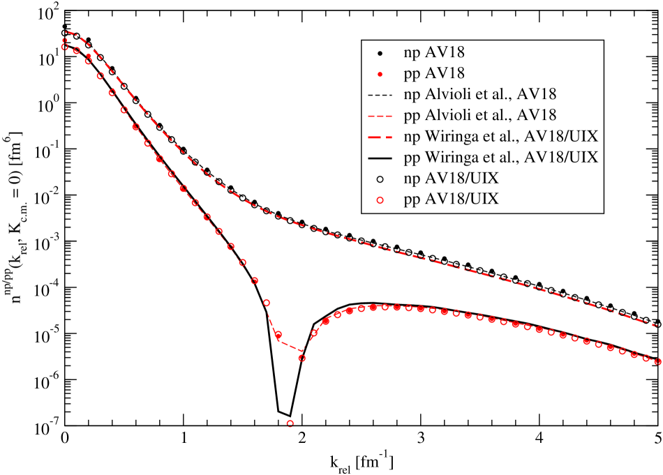
Figure 7: (Color online) The 2N momentum distributions $n^{np/pp}(k_{rel},K_{c.m.}=0)$, calculated using the AV18 and the AV18/UIX interaction models. The present results are shown as dots, while the previous studies of Refs. Alv13 ; Alv16 and Ref. Wir_web are shown as dashed or continuous lines.

We then move to the $n^{np/pp}(k_{rel})$ 2N momentum distribution as function of $K_{c.m.}^{+}$ (see Eq. (23)). The results for the AV18/UIX are shown in Fig. 8, from which we can conclude that contributions from $K_{c.m.}^{+}$ larger than approximately 5 fm^-1 are not significant. We also note, in passing, that for $K_{c.m.}^{+}=1.5$ fm^-1, the AV18 and AV18/UIX results are very close to each other.

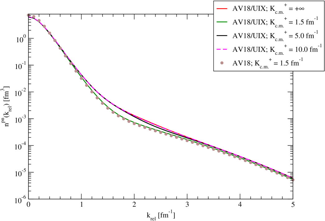
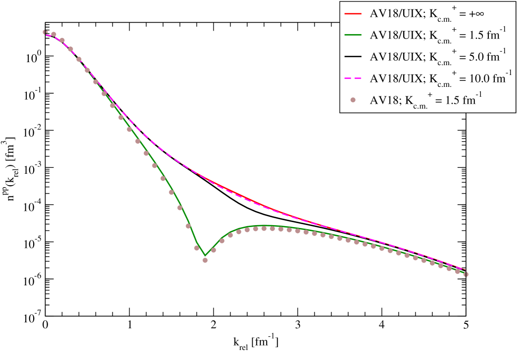
Figure 8: (Color online) The 2N momentum distributions $n^{np}(k_{rel})$ (left panel) and $n^{pp}(k_{rel})$ (right panel) as function of $K_{c.m.}^{+}$ (see Eq. (23)), calculated using the AV18/UIX potential. For $K_{c.m.}^{+}=1.5$ fm^-1 we show also the results obtained with the AV18 2N only potential.

Next we explore the model-dependence of the 2N momentum distributions, by repeating the calculations using the CDBonn potential without or with the TM 3N force. In Figs. 9 and 10 we show the results for the $n^{np/pp}(k_{rel},K_{c.m.}=0)$ and for the $n^{np/pp}(k_{rel})$ as function of $K_{c.m.}^{+}$, respectively. The figures reveal that: (i) the results with CDBonn/TM and those with AV18/UIX are substantially different from each other, especially in the high-$k_{rel}$ tails, confirming what we mentioned earlier while recalling the findings of Ref. src2015 ; (ii) the 3N force contributions are again barely appreciable on the plot (which are on a logarithmic scale); (iii) the $K_{c.m.}^{+}$-dependence in the CDBonn/TM case is very similar to the one seen in the AV18/UIX case.

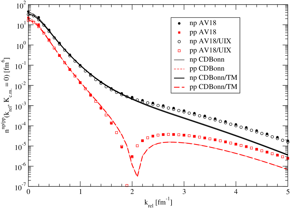
Figure 9: (Color online) The 2N momentum distributions $n^{np/pp}(k_{rel},K_{c.m.}=0)$, calculated using the AV18, AV18/UIX, CDBonn and CDBonn/TM 2N and 3N interaction models. The thin and think lines are on top of each other and can barely be distinguished.

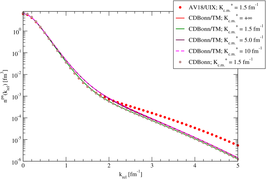
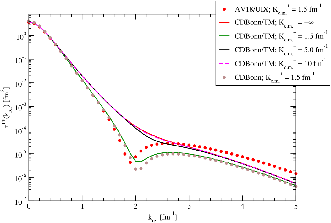
Figure 10: (Color online) The 2N momentum distributions $n^{np}(k_{rel})$ (left panel) and $n^{pp}(k_{rel})$ (right panel) as function of $K_{c.m.}^{+}$ (see Eq. (23)), calculated using the CDBonn/TM potential. For $K_{c.m.}^{+}=1.5$ fm^-1 we show also the results obtained with the CDBonn 2N only potential and the AV18/UIX potential, already presented in Fig. 8.

An important issue in the considerations of SRC is the behavior of $n^{np}(k_{rel})$ in nuclei as compared with the same quantity in the deuteron ($n^{np}_{d}(k_{rel})$). This is because a highly correlated $np$ pair in a nucleus is expected to exhibit a behavior similar to the pair in the deuteron. We proceed to calculate the integrated SRC-probabilities defined as

$$N_{N_{1}N_{2}}^{BB} = 4\pi\int_{0}^{\infty}n^{N_{1}N_{2}}(k_{rel},K_{c.m.}=0)k_{rel}^{2}\,dk_{rel}\ ,$$ (24)

$$N_{N_{1}N_{2}}^{SRC,BB} = 4\pi\int_{k_{rel}^{-}}^{\infty}n^{N_{1}N_{2}}(k_{rel},K_{c.m.}=0)k_{rel}^{2}\,dk_{rel}\ ,$$ (25)

$$N_{N_{1}N_{2}}^{SRC}(k_{rel}^{-}) = 4\pi\int_{k_{rel}^{-}}^{\infty}n^{N_{1}N_{2}}(k_{rel})k_{rel}^{2}\,dk_{rel}\ ,$$ (26)

$$N_{N_{1}N_{2}} = 4\pi\int_{0}^{\infty}n^{N_{1}N_{2}}(k_{rel})k_{rel}^{2}\,dk_{rel}\equiv N_{N_{1}N_{2}}^{SRC}(k_{rel}^{-}=0)\ ,$$ (27)

where we have used $k_{rel}^{-}=1.5$ fm^-1. These equations are the same as in Ref. Alv13 . For convenience, we will continue to refer to these integrated quantities as probabilities. A more accurate description of, for instance, $N_{N_{1}N_{2}}^{BB}$ would be the number of back-to-back $N_{1}N_{2}$ pairs after integration of the pair relative momentum.

The results for the different potential models used so far are shown in Table 6, from which we can conclude that the 3N force contributions are small also for the integrated quantities. However, model-dependence is strong, especially for $N^{SRC,BB}$ and $N^{SRC}(k_{rel}^{-})$. This large model-dependence might have impact on the extraction of SRC probabilities from $(e,e^{\prime}p)$ experiments, if not properly taken into account.

Table 6: The integrated $np$ and $pp$ SRC-probabilities, as defined in Eqs. (24)–(27), obtained with the various potential models, i.e. AV18, CDBonn, AV18/UIX and CDBonn/TM. For the $np$ case, we report in the last two lines labelled AV18 - d and CDBonn - d the deuteron results of Ref. src2015 .

	$N_{1}N_{2}=np$				$N_{1}N_{2}=pp$
	$N^{BB}$	$N^{SRC,BB}$	$N^{SRC}(k_{rel}^{-})$	$N$	$N^{BB}$	$N^{SRC,BB}$	$N^{SRC}(k_{rel}^{-})$	$N$
AV18	6.922	0.241	0.093	1.997	2.194	0.009	0.026	0.998
AV18/UIX	5.751	0.210	0.106	1.997	1.897	0.009	0.031	0.999
CDBonn	6.552	0.171	0.060	1.997	2.078	0.005	0.012	0.999
CDBonn/TM	5.931	0.157	0.063	1.998	1.924	0.005	0.014	0.998
AV18 - d			0.042
CDBonn - d			0.032

We now turn our attention to the 2N momentum distributions obtained with the 2N chiral potentials without or with the 3N forces, obtained as discussed in Sec. III.1. We begin with studying the order-by-order pattern, using the $\Lambda=500$ MeV cutoff as an example. The results obtained with the other values of $\Lambda$ display a similar behaviour. In the left panel of Fig. 11 we show the BB $np$ momentum distribution $n^{np}(k_{rel},K_{c.m.}=0)$ obtained using only the 2N force at LO, NLO, N2LO, N3LO and N4LO. In the right panel, we present the results for $n^{np}(k_{rel},K_{c.m.}=0)$ including the 3N force, with LECs obtained from Table 2 (model I) and 3 (model II), respectively. By inspection of the figures, we can conclude that the LO curve has a the distinct behavior at small $k_{rel}$ compared with the other curves, which suggests that the asymptotic part of the wave function at LO is significantly different than at the higher orders. Furthermore, the 3N force contribution is very small, and therefore the difference between the 3N force model is not visible. Finally, the N3LO and N4LO curves are very similar up to $k_{rel}\simeq 2.2$ fm^-1, indicating satisfactory order-by-order convergence at least in the region where the distributions still have non-negligible size. In Fig. 12 we show the corresponding BB $pp$ momentum distributions. As we can see, the same remarks apply in the $pp$ case as well.

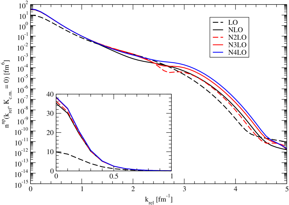
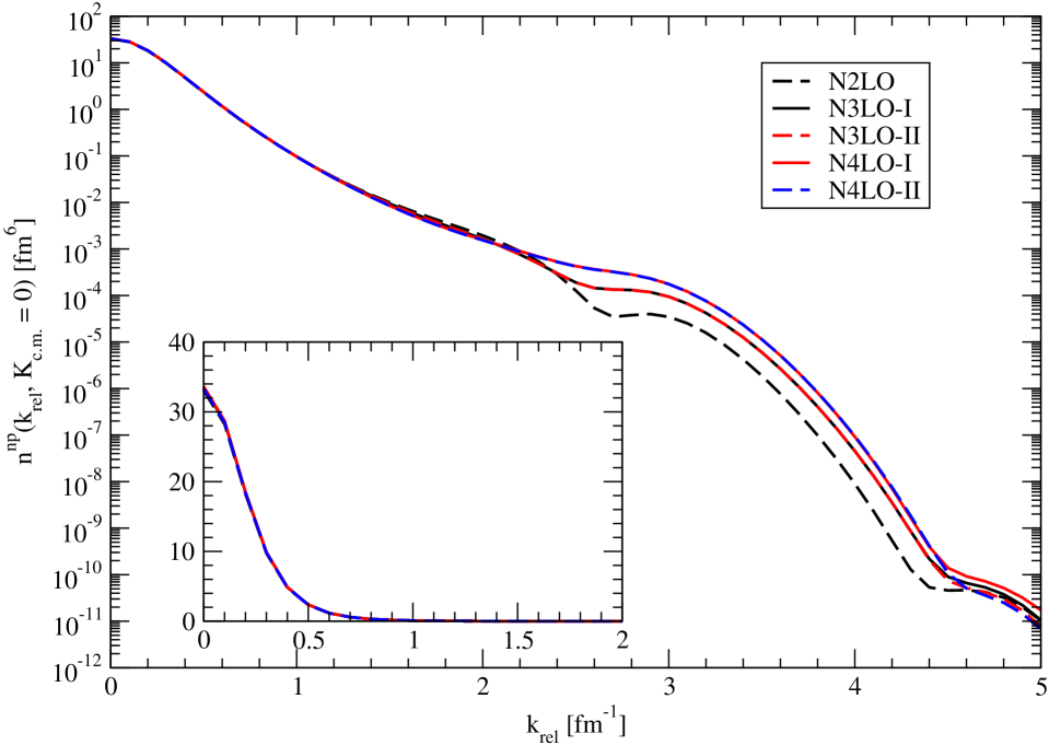
Figure 11: (Color online) The $np$ momentum distributions $n^{np}(k_{rel},K_{c.m.}=0)$, calculated using only 2N (left panel) and 2N+3N (right panel) chiral interactions, with $\Lambda=500$ MeV. The different chiral orders are labelled as in the text. On the right panel, we indicate with “I” and “II” the results obtained using the LECs of Table 2 and 3, respectively.

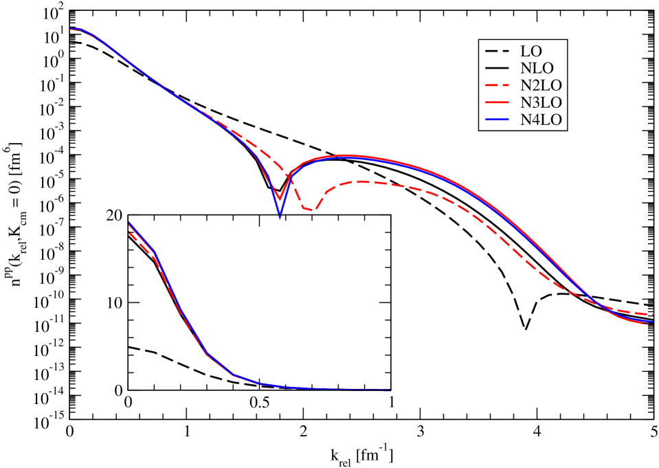
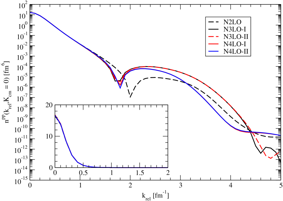
Figure 12: Same as Fig. 11 but for the $pp$ pair.

The BB 2N momentum distributions $n^{np}(k_{rel},K_{c.m.}=0)$ and $n^{pp}(k_{rel},K_{c.m.}=0)$ calculated with and without 3N interaction, at different chiral order and for different values of the cutoff $\Lambda$, are shown in Figs. 13 and 14, respectively. The results for the 2N momentum distributions $n^{np/pp}(k_{rel},K_{c.m.}^{+})$ for $K_{c.m.}^{+}=+1.5$ fm^-1 and $K_{c.m.}^{+}=+\infty$ are shown in Figs. 15, 16, 17 and 18. By inspection of all the figures we can conclude that we have essentially no cutoff dependence below $k_{rel}\simeq 2.2-2.5$ fm^-1, and increasingly strong cutoff dependence above it. Furthermore, the 3N force contributions are visible only for $k_{rel}\geq 3.0-3.5$ fm^-1. Note, however, that above $k_{rel}\simeq 2.5$ fm^-1 all momentum distributions are so small that the differences are of no practical relevance, see next.

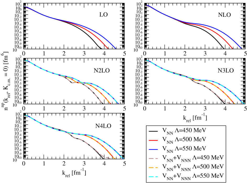
Figure 13: (Color online) The $np$ momentum distributions $n^{np}(k_{rel},K_{c.m.}=0)$, calculated using only 2N (solid lines) and 2N+3N (dashed lines) chiral interactions, at different chiral order and for three values of the cutoff $\Lambda=450,500,550$ MeV. The LECs of the 3N interaction are those of Table 3.

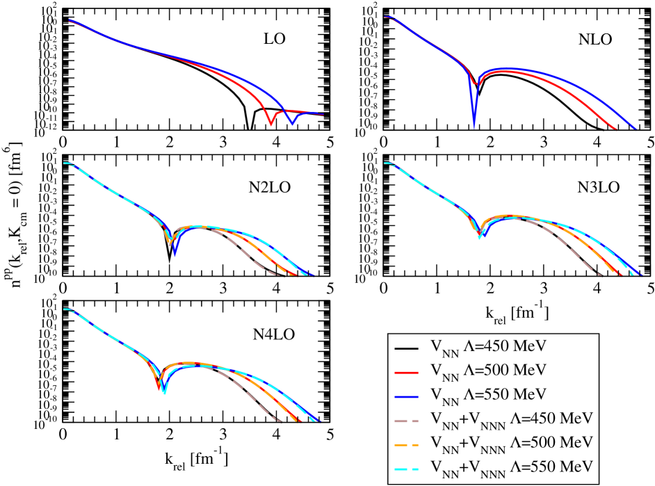
Figure 14: Same as Fig. 13 but for the $pp$ pair.

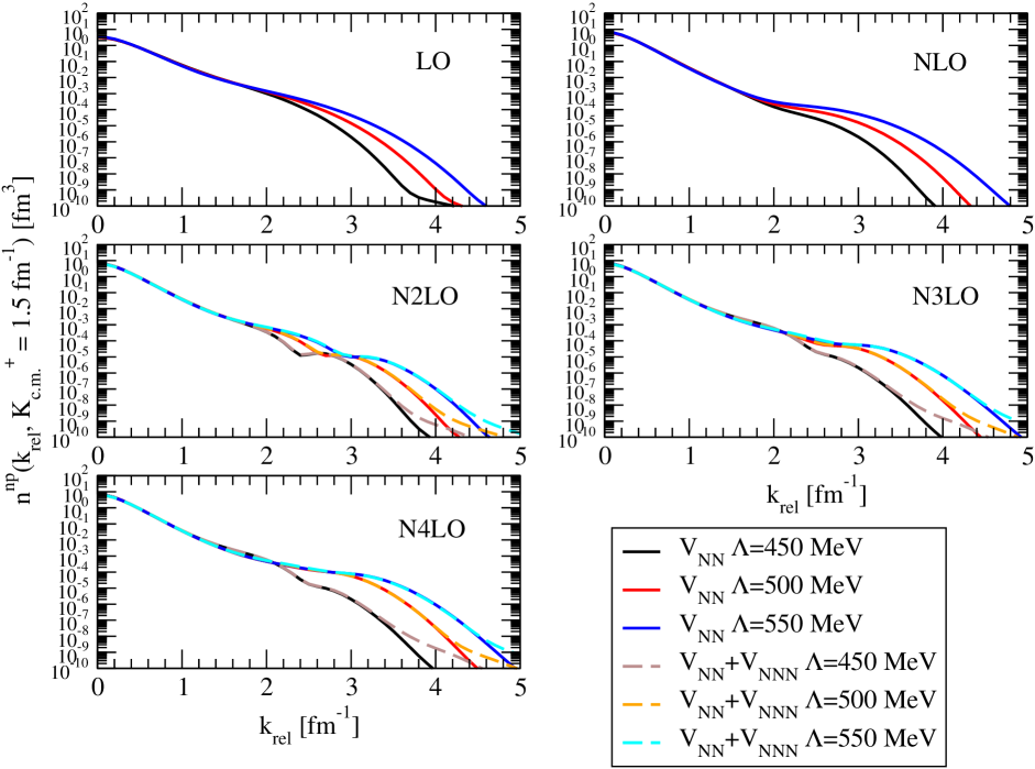
Figure 15: (Color online) The 2N momentum distributions $n^{np}(k_{rel},K_{c.m.}^{+})$ for $K_{c.m.}^{+}=+1.5$ fm^-1, calculated using only 2N (solid lines) and 2N+3N (dashed lines) chiral interactions, at different chiral order and for three values of the cutoff $\Lambda=450,500,550$ MeV. The LECs of the 3N interaction are those of Table 3.

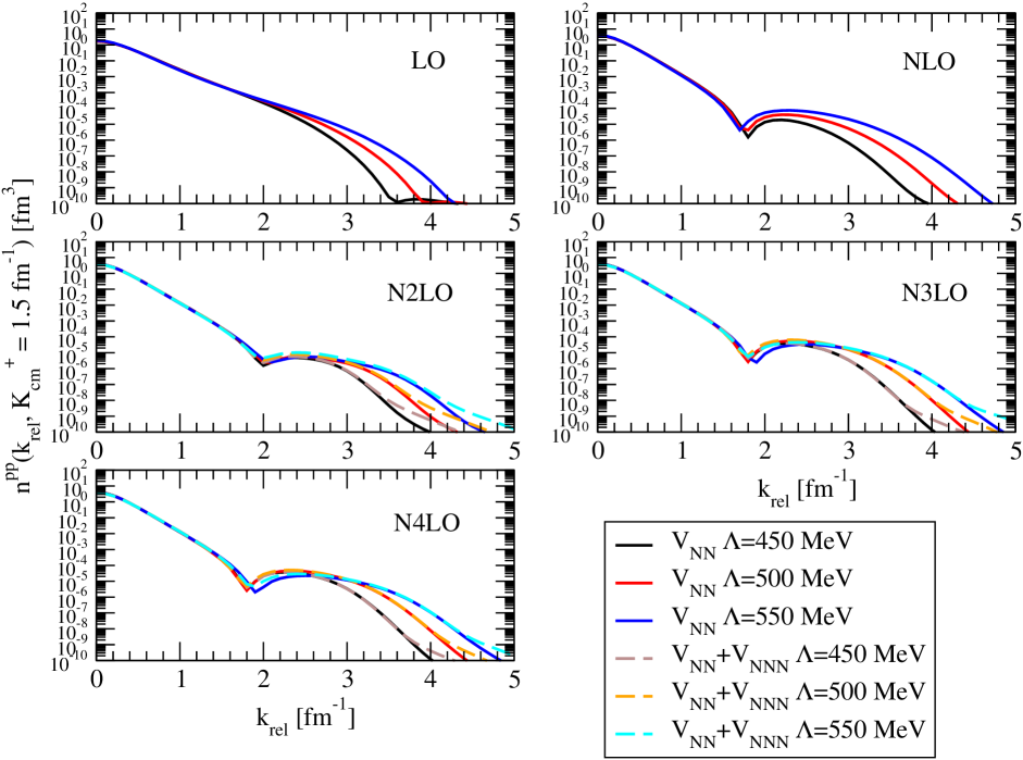
Figure 16: Same as Fig. 15 but for the $pp$ pair.

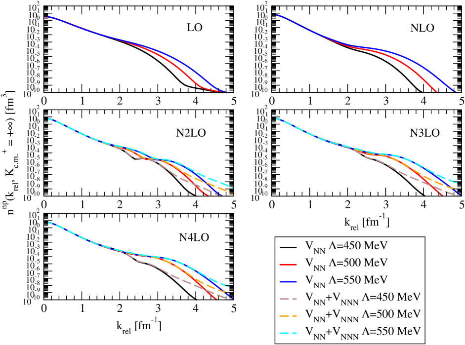
Figure 17: Same as Fig. 15 but for $K_{c.m.}^{+}=+\infty$.

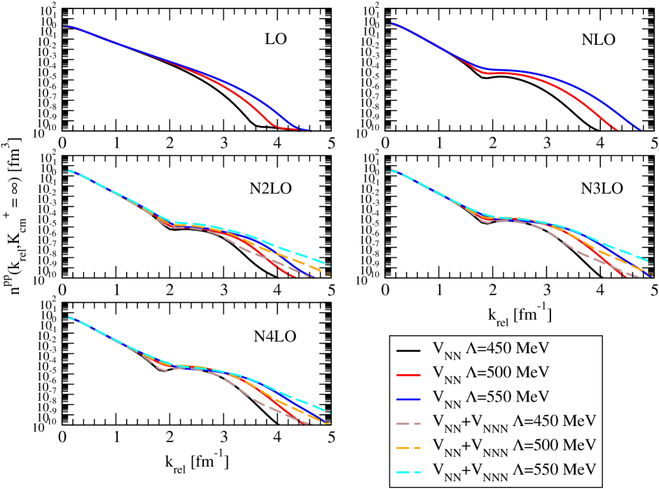
Figure 18: Same as Fig. 17 but for the $pp$ pair.

Calculating the integrated SRCs as defined in Eqs. (24)–(27), we obtain the values displayed in Tables 7 and 8 for $np$ and $pp$ SRCs, respectively. For these “observables”, as well, we find that order-by-order convergence is satisfactory and cutoff dependence is weak. This implies that the contributions from the region $k_{rel}\geq 2.2$ fm^-1 are essentially negligible.

Table 7: The integrated $np$ SRC-probabilities, as defined in Eqs. (24)–(27), obtained with chiral potentials, at different chiral orders, for different values of the cutoff $\Lambda$, 450, 500 and 550 MeV, also with the inclusion of the 3N force (lines labelled N2LO/N2LO at N2LO, N3LO/N3LO-I and N3LO/N3LO-I at N3LO, N4LO/N4LO-I and N4LO/N4LO-I at N4LO). The labels “I” and “II” refer to the LECs of Table 2 or 3, respectively.

	$N^{BB}$			$N^{SRC,BB}$			$N^{SRC}(k_{rel}^{-})$			$N$
Model/$\Lambda$ [MeV]	450	500	550	450	500	550	450	500	550	450	500	550
LO	2.731	2.829	3.051	0.094	0.120	0.144	0.089	0.112	0.126	1.999	1.999	1.998
NLO	5.896	6.054	6.458	0.047	0.066	0.096	0.016	0.024	0.037	1.998	1.998	1.997
N2LO	5.977	6.127	6.236	0.087	0.118	0.141	0.029	0.038	0.045	1.998	1.997	1.997
N2LO/N2LO	5.844	5.831	5.827	0.086	0.114	0.135	0.030	0.040	0.050	1.998	1.998	1.998
N3LO	6.443	6.314	6.317	0.131	0.112	0.122	0.039	0.039	0.044	1.997	1.997	1.997
N3LO/N3LO-I	5.823	5.884	5.907	0.121	0.107	0.117	0.042	0.043	0.051	1.998	1.998	1.998
N3LO/N3LO-II	5.817	5.865	5.890	0.121	0.107	0.117	0.042	0.043	0.050	1.998	1.998	1.998
N4LO	6.360	6.345	6.266	0.125	0.119	0.129	0.038	0.042	0.047	1.997	1.997	1.998
N4LO/N4LO-I	5.823	5.911	5.915	0.116	0.114	0.125	0.041	0.047	0.054	1.998	1.998	1.998
N4LO/N4LO-II	5.809	5.868	5.857	0.116	0.113	0.123	0.040	0.045	0.051	1.998	1.998	1.998

Table 8: Same as Table 7 but for the $pp$ pair.

	$N^{BB}$			$N^{SRC,BB}$			$N^{SRC}(k_{rel}^{-})$			$N$
Model/$\Lambda$ [MeV]	450	500	550	450	500	550	450	500	550	450	500	550
LO	1.049	1.087	1.165	0.016	0.020	0.023	0.030	0.040	0.045	0.999	0.999	0.999
NLO	1.976	2.014	2.109	0.002	0.004	0.009	0.002	0.004	0.010	0.999	0.999	0.998
N2LO	1.975	2.009	2.036	0.002	0.002	0.003	0.003	0.004	0.005	0.998	0.998	0.998
N2LO/N2LO	1.943	1.935	1.932	0.002	0.002	0.002	0.003	0.004	0.006	0.999	0.998	0.998
N3LO	2.083	2.061	2.060	0.004	0.007	0.006	0.003	0.007	0.009	0.998	0.998	0.998
N3LO/N3LO-I	1.928	1.952	1.958	0.004	0.007	0.006	0.004	0.009	0.011	0.998	0.999	0.999
N3LO/N3LO-II	1.927	1.948	1.953	0.004	0.007	0.006	0.004	0.008	0.011	0.998	0.999	0.999
N4LO	2.064	2.070	2.048	0.004	0.005	0.004	0.004	0.008	0.009	0.998	0.998	0.998
N4LO/N4LO-I	1.929	1.960	1.962	0.004	0.006	0.004	0.004	0.009	0.012	0.998	0.999	0.999
N4LO/N4LO-II	1.926	1.949	1.945	0.004	0.005	0.004	0.004	0.009	0.010	0.998	0.999	0.999

Earlier in the paper, we noted that the momentum distributions we calculated with chiral interactions die out at a faster rate than those obtained with phenomenological potentials. In Sect. III.2, we pointed out that such feature may be expected given the softer nature of chiral forces. While this is a correct observation within the spectrum of interactions considered here, it is important to note that the chiral nature of an interaction does not necessarily bring additional softness. To support this statement, we refer to Ref. loc_chi , where predictions for 1N and 2N momentum distributions in $A\leq$16 are shown. In that work it is concluded that, when local chiral interactions are employed, the resulting momentum distributions are consistent with those obtained from local phenomenological potentials. In fact, the local 2N chiral interactions (at N2LO) applied in Ref. loc_chi and developed in Refs. Gez+13 ; Gez+14 predict a $D$-state probability for the deuteron ranging between 5.5 and 6.1%, values which are typical for the “hardest” local potentials.

Therefore, once again, the local vs. non-local nature of the 2N force (by far the largest contribution to the 1N and 2N momentum distributions, as we have observed on several occasions), is a major factor in determining the characteristics of momentum distributions in nuclei and, particularly, their short-range part.

IV Conclusions and outlook

We have presented predictions for 1N and 2N momentum distributions in the deuteron and in ³He. We have employed state-of-the-art chiral 2N potentials (with or without the leading chiral 3N force) and also, for the purpose of comparison and validation of our tools, older potentials plus 3N force, either fully phenomenological or based on meson theory. A main motivation was to explore the short-range few-nucleon dynamics as predicted by these diverse interactions. One of our findings is that, regardless the 2N force model, the contribution from 3N forces is always very weak.

We have also quantified and pointed out, as appropriate, any significant model dependence of SRCs. We noted that SRCs in the lightest few-nucleon systems may impact the extraction of (semi-)empirical information for heavier nuclei, all the way to extrapolations in nuclear matter. In fact, for heavier systems, integrated SRC probabilities have been extracted from empirical information together with some model-dependent assumptions CLAS ; CLAS2 .

Although potentials based on chiral EFT may be expected to produce weaker SRC than purely phenomenological or meson-exchange ones, on several occasions the discussion of model dependence led back to considerations of locality vs. non-locality of the underlying 2N force, rather than “chiral” vs. “non-chiral”. We find this to be an important issue, extensively debated in the literature of the 1990’s MSS96 ; Polls98 ; MP99 and now re-emerging in the light of new stimulating discussions.

The 2N potentials considered here have an established success record with low-energy predictions, such as the structure of light and medium-mass nuclei as well as the properties of nuclear matter. But, as shown above, they differ considerably in their high-momentum components. Thus, one may raise the question of whether the predictions of these potentials in the high-momentum regions probed by the JLab measurements are reliable or, to a certain extent, arbitrary. Note that there is no physical reason why the off-shell behavior of, say, AV18, should be preferable as compared to other potentials. In fact, on fundamental grounds off-shell behavior is not observable and, therefore, “empirical” information related to the (as we have shown, very diverse) off-shell nature of the potentials is highly model dependent. To stress this point even more: 2N potentials which are known as $V_{low-k}$ BKS03 are typically cut off between 1.5 and 2 fm^-1 and, thus, produce essentially zero SRC. However, these low-momentum interactions are highly successful in ab initio nuclear structure calculations and, thus, are valid 2N potentials.

Considering all of the above, our investigation prompts us to conclude the following: since SRC “empirical” information is in part based on the high-momentum behavior of a specific 2N interaction CLAS ; CLAS2 , the reported information should be understood as carrying very large uncertainty, and such uncertainty should be quantified and stated.

In the near future, we plan to extend our study to triton and ⁴He. In both the $A=3$ nuclei, we will look into other interesting quantities which are related to momentum distributions and SRC, such as the ratio of $pp$ to $pn$ 2N momentum distributions vs. $k_{rel}$, and the ration of $pp$ to $np$ pairs in the back-to-back case. For ⁴He, the ratio of $pp$ to $np$ pairs is also of interest, as information on this ratio as extracted from high momentum-transfer triple-coincidence measurements of ⁴He($e,e^{\prime}\;p\;N$) is reported in Ref. Korover . Similar measurements are present in Ref. Sub+2008 for ²⁷Al, and in Ref. Hen+2014 for ²⁰⁸Pb.

References

- (1) K.S. Egiyan et al., Phys. Rev. Lett. 96, 082501 (2006), and references therein.
- (2) K.S. Egiyan et al., CLAS-NOTE 2005-004, 2005, www1.jlab.org/ul/Physics/Hall-B/clas.
- (3) K.S. Egiyan et al., Phys. Rev. C 68, 014313 (2003).
- (4) Michael McGauley and Misak M. Sargsian, arXiv:1102.3973v3 (2012).
- (5) E. Piasetzky et al., Phys. Rev. Lett. 97, 162504 (2006).
- (6) K.S. Egiyan et al., Phys. Rev. Lett. 96, 082501 (2006).
- (7) F. Sammarruca, Phys. Rev. C 90 , 064312 (2014); and references therein.
- (8) A. Tang et al., Phys. Rev. Lett. 90, 042301 (2003).
- (9) I. Korover et al. (Jefferson Lab Hall A Collaboration), Phys. Rev. Lett. 113, 022501 (2014).
- (10) R. Shneor et al. (Jefferson Lab Hall A Collaboration), Phys. Rev. Lett. 99, 072501 (2007).
- (11) R. Subedi et al., Science 320, 1476 (2008).
- (12) H. Baghdasaryan et al. (CLAS Collaboration), Phys. Rev. Lett. 105, 222501 (2010).
- (13) F. Sammarruca, Phys. Rev. C 92, 044003 (2015).
- (14) R.B. Wiringa, V.G.J. Stoks, and R. Schiavilla, Phys. Rev. C 51, 38 (1995).
- (15) V.G.J. Stoks, R.A.M. Klomp, C.P.F. Terheggen, and J.J. de Swart, Phys. Rev. C 49, 2950 (1994).
- (16) R. Machleidt, Phys. Rev. C 63, 024001 (2001).
- (17) D.R. Entem and R. Machleidt, Phys. Rev. C 68, 041001, (2003).
- (18) E. Marji, A. Canul, Q. MacPherson, R. Winzer, Ch. Zeoli, D.R. Entem, and R. Machleidt, Phys. Rev. C 88, 054002 (2013).
- (19) R. Machleidt and D.R. Entem, Phys. Rep. 503, 1 (2011).
- (20) R. Machleidt, F. Sammarruca, and Y. Song, Phys. Rev. C 53, 1483 (1996).
- (21) A. Polls, H. Müther, R. Machleidt, and M. Hjorth-Jensen, Phys. Lett. B 432, 1 (1998).
- (22) H. Müther and A.Polls, Phys. Rev. C 61, 014304 (1999).
- (23) D.R. Entem, R. Machleidt, and Y. Nosyk, Phys. Rev. C 96, 024004 (2017).
- (24) M. Hoferichter, J. Ruiz, de Elvira, B. Kubis, and U.-G. Meissner, Phys. Rev. Lett. 115, 192301 (2015); Phys. Rep. 625, 1 (2016).
- (25) B.S. Pudliner, V.R. Pandharipande, J. Carlson, and R.B. Wiringa, Phys. Rev. Lett. 74, 4396 (1995).
- (26) S.A. Coon and H.K. Han, Few-Body Systems 30, 131 (2001).
- (27) M. Alvioli, C. Ciofi degli Atti, L.P. Kaptari, C.B. Mezzetti, and H. Morita, Phys. Rev. C 87, 034603 (2013).
- (28) M. Alvioli, C. Ciofi degli Atti, and H. Morita, Phys. Rev. C 94, 044309 (2016).
- (29) R.B. Wiringa, R. Schiavilla, S. Pieper, and J. Carlson, Phys. Rev. C 89, 024305 (2014); R.B. Wiringa, https://www.phy.anl.gov/theory/research/momenta2/
- (30) M. Viviani et al., Few-Body Syst. 39, 159 (2006)
- (31) A. Kievsky et al., J. Phys. G 35, 063101 (2008)
- (32) L.E. Marcucci, A. Kievsky, S. Rosati, R. Schiavilla, and M. Viviani, Phys. Rev. Lett. 108, 052502, (2012); Erratum: Phys. Rev. Lett. 121, 049901 (2018).
- (33) F. Sammarruca, L.E. Marcucci, L. Coraggio, J.W. Holt, N. Itaco, and R. Machleidt, arXiv:1807.06640.
- (34) H. Krebs, A. Gasparyan, and E. Epelbaum, Phys. Rev. C 85, 054006 (2012).
- (35) J.G. Van der Corput, Akademie van Wetenschappen 38, 813 (1935).
- (36) L. L. Frankfurt, M.I. Strikman, D.B. Day, and M. Sargsyan, Phys. Rev. C 48, 2451 (1993).
- (37) C. Ciofi degli Atti and S. Simula, Phys. Rev. C 53, 1689 (1996).
- (38) A. Nogga et al., Phys. Rev. C 67, 034004 (2003).
- (39) V. Bernard, E. Epelbaum, H. Krebs, and Ulf-G. Meissner, Phys. Rev. C 77, 064004 (2008); Phys. Rev. C 84, 054001 (2011).
- (40) H. Krebs, A. Gasparyan, and E. Epelbaum, Phys. Rev. C 85, 054006 (2012); Phys. Rev. C 87, 054007 (2013).
- (41) L. Girlanda, A. Kievsky, and M. Viviani, Phys. Rev. C 84, 014001 (2011).
- (42) E. Piasetzky, O. Hen, and L.B. Weinstein, AIP Conf. Proc. 1560, 355 (2013).
- (43) D. Lonardoni, S. Gandolfi, X.B. Wang, and J. Carlson, arXiv:1804.08027.
- (44) A. Gezerlis, I. Tews, E. Epelbaum, S. Gandolfi, K. Hebeler, A. Nogga, and A. Schwenk, Phys. Rev. Lett 111, 032501 (2013).
- (45) A. Gezerlis, I. Tews, E. Epelbaum, M. Freunek, S. Gandolfi, K. Hebeler, A. Nogga, and A. Schwenk, Phys. Rev. C 90, 054323 (2014).
- (46) S.K. Bogner, T.T.S. Kuo, and A. Schwenk, Phys. Rep. 386, 1 (2003).
- (47) R. Subedi et al., Science 320, 1476 (2008).
- (48) O. Hen et al., Science 346, 614 (2014).