Violation of generalized Bell inequality and its optimal measurement settings

Abstract

We provide a method to describe quantum nonlocality for $n$-qubit systems. By treating the correlation function as an $n$-index tensor, we derive a generalized Bell inequality. Taking generalized Greenberger-Horne-Zeilinger (GHZ) state for example, we calculate quantum prediction under a series of measurement settings involving various angle parameters. We reveal the exact relationship between quantum prediction and the angle parameters. We show that there exists a set of optimal measurement settings and find the corresponding maximal quantum prediction for $n$-qubit generalized GHZ states. As an example, we consider an interesting situation involving only two angle parameters. Finally, we obtain a criterion for the violation of the generalized Bell inequality.

I Introduction

To demonstrate the nonlocal quantum correlation of quantum system, in 1964, Bell Bell1964 proved that quantum predictions are incompatible with the local hidden variable (LHV) model by a simple logical contradiction. Inspired by this seminal paper, Clauser et al. CHSH1969 derived a correlation inequality, namely Clauser-Horne-Shimony-Holt (CHSH) inequality, which provides a way of experimentally testing the LHV theory. Then, a series of multipartite Bell-type inequalities have been proposed Mermin1990 ; Ardehali1992 ; BK1993 ; WW2001 ; ZB2002 ; WYKO2007PRA75-032332 ; GSDRS2009 ; LF2012 ; WZCG2013 ; DHYG2015CPB ; HDYG2015EPL , where Werner-Wolf-Żukowski-Brukner (WWZB) inequalities WW2001 ; ZB2002 are the most important because of the properties of investigating the possible connections between quantum nonlocality and entanglement for $n$-qubit systems. For two-qubit systems, the theorem of Gisin G91 ; GP92 states that all pure entangled states violate the CHSH inequality. Then, Chen et al. CWKO2004 generalized Gisin’s theorem to three-qubit system and showed that all three-qubit generalized Greenberger-Horne-Zeilinger (GHZ) states violate a Bell inequality for probabilities. On the other hand, given a set of standard Bell experiment settings involving two dichotomic observables for each position, there exist pure $n$-qubit entangled states that do not violate any Bell inequality ZBLW2002 . By now it is an open question whether Gisin’s theorem can be generalized to an arbitrary $n$-qubit system BCPSW2014 . In any event, the key to investigating Bell inequalities with multipartite correlation functions is to find a set of optimal measurement settings.

Optical quantum systems DDI2006 ; Kok2007 ; Pan2012 ; LDJW2007 ; AGACVMC2012 ; CM2014 ; LDQ2015 ; KNM2017 are prominent candidates for testing nonlocal quantum correlations, since multiphoton entanglement, interferometry and measurement are relatively easy to perform in experiments, as long as the number of photons is not very large. In 2001, Weinfurter and Żukowski WZ2001 proposed a scheme to produce a superposition of four-photon GHZ state with a product state of two Bell states and investigated the features of this state by constructing a Bell-type inequality. By introducing a set of polarization correlation measurements, it has been shown that with a given set of measurement settings the maximal violation of the Bell-type inequality is $4\sqrt{2}/3$. Later, with this method, Li and Kobayashi LK2004 investigated another four-photon superposition state, and more recently, Ding et al. DHYG2017-4-photon discussed a class of generic superposition of four-photon entangled states with a tunable angle parameter. Of course, a natural question is whether or not the given settings WZ2001 ; LK2004 ; DHYG2017-4-photon are optimal or unique.

In this paper, we investigate quantum nonlocality for $n$-qubit entangled states. We first describe a method of treating correlation function as an $n$-index tensor and then derive a generalized Bell inequality. Under a set of measurement settings involving various angle parameters, we calculate quantum prediction of generalized GHZ states and show the exact relationship between quantum prediction and the angle parameters. We demonstrate that there is a set of optimal measurement settings and obtain the corresponding maximal quantum prediction for $n$-qubit generalized GHZ states. We analyze the interesting situation involving only two angle parameters in details. Finally, as an important application, a criterion for the violation of the generalized Bell inequality is provided.

II A generalized Bell inequality for $n$-qubit system

In LHV theory BCPSW2014 , a correlation function represents an average over many runs of experiment. An $n$-partite correlation function for two alternative dichotomic measurements is generally given by

$$E_{\textrm{LHV}}(\phi_{1}^{k_{1}},\phi_{2}^{k_{2}},\cdots,\phi_{n}^{k_{n}})=\int d\lambda\rho(\lambda)I_{1}(\phi_{1}^{k_{1}},\lambda)I_{2}(\phi_{2}^{k_{2}},\lambda)\cdots I_{n}(\phi_{n}^{k_{n}},\lambda),$$ (1)

where $\lambda$ is a hidden variable and $\rho(\lambda)$ is the probability distribution function, $\phi_{i}^{k_{i}}$, $(k_{i}=0,1)$ indicates the local phase angle at site $i$, and $I_{i}(\phi_{i}^{k_{i}},\lambda)=\pm 1$, $i=1,2,\cdots,n$, represents the predetermined binary outcomes of the measurements. As described by Weinfurter and Żukowski WZ2001 , one can treat the four-photon correlation function as a four-index tensor. Here we consider an $n$-index tensor which is obtained by taking the form of a tensor product of $n$ two-dimensional real vectors $\textbf{v}_{i}^{\lambda}=(I_{i}(\phi_{i}^{0},\lambda),I_{i}(\phi_{i}^{1},\lambda))$, $i=1,2,\cdots,n$. That is, we define a tensor for $n$-partite system as

$$\hat{E}_{\textrm{LHV}}=\int d\lambda\rho(\lambda)\textbf{v}_{1}^{\lambda}\otimes\textbf{v}_{2}^{\lambda}\otimes\cdots\otimes\textbf{v}_{n}^{\lambda}.$$ (2)

Choose two orthogonal unit vectors

$$\textbf{v}_{i}^{0}=(1,0),~{}~{}~{}~{}\textbf{v}_{i}^{1}=(0,1).$$ (3)

Since each of the vectors $\textbf{v}_{i}^{\lambda}$ can be written as $\sum_{k_{i}=0,1}I_{i}(\phi_{i}^{k_{i}},\lambda)\textbf{v}_{i}^{k_{i}}$, one can simplify the correlation function as

$$\hat{E}_{\textrm{LHV}} = \sum_{k_{1},k_{2},\cdots,k_{n}=0,1}E_{\textrm{LHV}}(\phi_{1}^{k_{1}},\phi_{2}^{k_{2}},\cdots,\phi_{n}^{k_{n}})\textbf{v}_{1}^{k_{1}}\otimes\textbf{v}_{2}^{k_{2}}\otimes\cdots\otimes\textbf{v}_{n}^{k_{n}}.$$ (4)

Let $\textbf{A}_{i}^{0}=(1,1)$ and $\textbf{A}_{i}^{1}=(1,-1)$. Obviously,

$$\textbf{v}_{i}^{k_{i}}=\frac{1}{2}[\textbf{A}_{i}^{0}+(-1)^{k_{i}}\textbf{A}_{i}^{1}],~{}~{}~{}k_{i}=0,1,~{}~{}~{}i=1,2,\cdots,n.$$ (5)

The correlation function can be expressed as

$$\hat{E}_{\textrm{LHV}} = \frac{1}{2^{n}}\sum_{j_{1},j_{2},\cdots,j_{n}=0,1}\sum_{k_{1},k_{2},\cdots,k_{n}=0,1}(-1)^{\textbf{k}\centerdot\textbf{j}}$$ (6)

$$\times E_{\textrm{LHV}}(\phi_{1}^{k_{1}},\phi_{2}^{k_{2}},\cdots,\phi_{n}^{k_{n}})\textbf{A}_{1}^{j_{1}}\otimes\textbf{A}_{2}^{j_{2}}\otimes\cdots\otimes\textbf{A}_{n}^{j_{n}},$$

where $\textbf{k}=(k_{1},k_{2},\cdots,k_{n})$ and $\textbf{j}=(j_{1},j_{2},\cdots,j_{n})$. Let

$$c_{j_{1},j_{2},\cdots,j_{n}}=\frac{1}{2^{n}}\sum_{k_{1},k_{2},\cdots,k_{n}=0,1}(-1)^{\textbf{k}\centerdot\textbf{j}}E_{\textrm{LHV}}(\phi_{1}^{k_{1}},\phi_{2}^{k_{2}},\cdots,\phi_{n}^{k_{n}})$$ (7)

be the LHV correlation coefficients. Then we have

$$\hat{E}_{\textrm{LHV}} = \sum_{j_{1},j_{2},\cdots,j_{n}=0,1}c_{j_{1},j_{2},\cdots,j_{n}}\textbf{A}_{1}^{j_{1}}\otimes\textbf{A}_{2}^{j_{2}}\otimes\cdots\otimes\textbf{A}_{n}^{j_{n}}.$$ (8)

Let $\textbf{A}_{i}^{2}=(-1,-1)$ and $\textbf{A}_{i}^{3}=(-1,1)$, then we can use the probability to describe $n$-partite correlation function (2) as

$$\hat{E}_{\textrm{LHV}}=\sum_{j_{1},j_{2},\cdots,j_{n}=0,1,2,3}p_{j_{1},j_{2},\cdots,j_{n}}\textbf{A}_{1}^{j_{1}}\otimes\textbf{A}_{2}^{j_{2}}\otimes\cdots\otimes\textbf{A}_{n}^{j_{n}},$$ (9)

where $p_{j_{1},j_{2},\cdots,j_{n}}$ is the probability of $\textbf{v}_{i}^{\lambda}$ being $\textbf{A}_{i}^{j_{i}},i=1,2,\cdots,n,j_{i}=0,1,2,3$, i.e., $p_{j_{1},j_{2},\cdots,j_{n}}$ is the probability of obtaining measurement outcomes $\textbf{A}_{1}^{j_{1}},\textbf{A}_{2}^{j_{2}},\cdots,\textbf{A}_{n}^{j_{n}}$. Obviously,

$$\sum_{j_{1},j_{2},\cdots,j_{n}=0,1,2,3}p_{j_{1},j_{2},\cdots,j_{n}}=1.$$

Note that $\textbf{A}_{i}^{j_{i}+2}=-\textbf{A}_{i}^{j_{i}}$ with $j_{i}=0,1$, we obtain

$$\hat{E}_{\textrm{LHV}} = \sum_{j_{1},j_{2},\cdots,j_{n}=0,1}(p_{j_{1},j_{2},\cdots,j_{n}}-p_{j_{1}+2,j_{2},\cdots,j_{n}}-\cdots-p_{j_{1},j_{2},\cdots,j_{n-1},j_{n}+2}$$ (10)

$$+p_{j_{1}+2,j_{2}+2,j_{3},\cdots,j_{n}}+\cdots-p_{j_{1}+2,j_{2}+2,j_{3}+2,j_{4},\cdots,j_{n}}-\cdots)\textbf{A}_{1}^{j_{1}}\otimes\textbf{A}_{2}^{j_{2}}\otimes\cdots\otimes\textbf{A}_{n}^{j_{n}}.$$

Compared with Eq.(8), one gets

$$c_{j_{1},j_{2},\cdots,j_{n}}= p_{j_{1},j_{2},\cdots,j_{n}}-p_{j_{1}+2,j_{2},\cdots,j_{n}}-\cdots-p_{j_{1},j_{2},\cdots,j_{n-1},j_{n}+2}+p_{j_{1}+2,j_{2}+2,j_{3},\cdots,j_{n}}+\cdots$$ (11)

$$-p_{j_{1}+2,j_{2}+2,j_{3}+2,j_{4},\cdots,j_{n}}-\cdots.$$

Then

$$\sum_{j_{1},j_{2},\cdots,j_{n}=0,1}|c_{j_{1},j_{2},\cdots,j_{n}}|\leq 1.$$ (12)

This inequality is derived from the natural generalization of the four-qubit correlation inequality WZ2001 to $n$-qubit systems. It is conventionally referred to as generalized Bell inequality, and can be used to test the LHV theory. It may be equivalent to WWZB inequality WW2001 ; ZB2002 and limits the total amount of correlation allowed for the LHV theory.

On the other hand, quantum mechanically, suppose a measurement, described by measurement operator

$$\{M_{x}=|m_{x},\phi_{x}\rangle\langle m_{x},\phi_{x}|,m_{x}=\pm 1\}$$ (13)

is performed upon $x$-port with a detector placed at the corresponding output station, where

$$|m_{x},\phi_{x}\rangle=\frac{1}{\sqrt{2}}(|0\rangle_{x}+m_{x}\text{e}^{-\text{i}\phi_{x}}|1\rangle_{x}),~{}~{}~{}x=1,2,\cdots,n,$$ (14)

$\phi_{x}$ is a local phase setting chosen by each of the observers and $m_{x}$ represents the possible measurement result.

Consider a standard quantum correlation test, in which each observer chooses between two dichotomic measurements; that is, for each site one can label phase angle $\phi_{x}^{k_{x}}$, $k_{x}=0,1$ and take $m_{x}=\pm 1$. For an $n$-qubit entangled state $|\psi_{n}\rangle$, the probability of outcomes $m_{1},m_{2},\cdots,m_{n}$ with the phase settings $\phi_{1}^{k_{1}},\phi_{2}^{k_{2}},\cdots,\phi_{n}^{k_{n}}$ labels $p(m_{1},m_{2},\cdots,m_{n}|\phi_{1}^{k_{1}},\phi_{2}^{k_{2}},\cdots,\phi_{n}^{k_{n}})$ and then the correlation function can be represented by

$$E_{\textrm{QM}}(\phi_{1}^{k_{1}},\phi_{2}^{k_{2}},\cdots,\phi_{n}^{k_{n}}) = \sum_{m_{1},m_{2},\cdots,m_{n}=\pm 1}p(m_{1},m_{2},\cdots,m_{n}|\phi_{1}^{k_{1}},\phi_{2}^{k_{2}},\cdots,\phi_{n}^{k_{n}})m_{1}m_{2}\cdots m_{n},$$ (15)

where the sum is over all possible runs of experiment. This set of operators is sufficient to describe the quantum correlation in contrast to the LHV case.

Similarly, the quantum correlation function can also be described by the $n$-fold tensor

$$\hat{E}_{\textrm{QM}} = \sum_{j_{1},j_{2},\cdots,j_{n}=0,1}q_{j_{1},j_{2},\cdots,j_{n}}\textbf{A}_{1}^{j_{1}}\otimes\textbf{A}_{2}^{j_{2}}\otimes\cdots\otimes\textbf{A}_{n}^{j_{n}},$$ (16)

where

$$q_{j_{1},j_{2},\cdots,j_{n}}=\frac{1}{2^{n}}\sum_{k_{1},k_{2},\cdots,k_{n}=0,1}(-1)^{\textbf{k}\centerdot\textbf{j}}E_{\textrm{QM}}(\phi_{1}^{k_{1}},\phi_{2}^{k_{2}},\cdots,\phi_{n}^{k_{n}})$$ (17)

are quantum correlation coefficients. Compared with the inequality (12) derived from the LHV correlation, once quantum prediction

$$\sum_{j_{1},j_{2},\cdots,j_{n}=0,1}|q_{j_{1},j_{2},\cdots,j_{n}}|$$ (18)

is greater than the classical limit value 1, which means that Bell inequality is violated and quantum nonlocal correlations of quantum system occurs.

III Quantum prediction for $n$-qubit generalized GHZ states

In a finite-dimensional Hilbert space, consider an $n$-qubit generalized GHZ state

$$|\psi_{n}\rangle = \alpha|00\cdots 0\rangle_{12\cdots n}+\beta|11\cdots 1\rangle_{12\cdots n},$$ (19)

where $\alpha$ and $\beta$ are respectively the complex parameters satisfying the normalization condition $|\alpha|^{2}+|\beta|^{2}=1$. A computation reveals that the quantum correlation function determined by the dichotomic measurement parameter settings $\{\phi_{1}^{k_{1}},\phi_{2}^{k_{2}},\cdots,\phi_{n}^{k_{n}}\}$ for the generalized GHZ state (19) is

$$E_{\textrm{QM}}(\phi_{1}^{k_{1}},\phi_{2}^{k_{2}},\cdots,\phi_{n}^{k_{n}}) = 2\text{Re}[\alpha\beta^{*}\text{e}^{-\text{i}(\phi_{1}^{k_{1}}+\phi_{2}^{k_{2}}+\cdots+\phi_{n}^{k_{n}})}].$$ (20)

Without loss of generality we suppose that $\alpha$ and $\beta$ are real. Then the quantum prediction is

$$\sum_{j_{1},j_{2},\cdots,j_{n}=0,1}|q_{j_{1},j_{2},\cdots,j_{n}}|=\frac{|\alpha\beta|}{2^{n-1}}\sum_{j_{1},j_{2},\cdots,j_{n}=0,1}|\sum_{k_{1},k_{2},\cdots,k_{n}=0,1}(-1)^{\textbf{k}\centerdot\textbf{j}}\text{Re}[\text{e}^{-\text{i}(\phi_{1}^{k_{1}}+\phi_{2}^{k_{2}}+\cdots+\phi_{n}^{k_{n}})}]|.$$ (21)

Let

$$\alpha_{l}=\frac{(\phi_{l}^{1}+\phi_{l}^{0})}{2},~{}~{}~{}~{}~{}\beta_{l}=\frac{(\phi_{l}^{1}-\phi_{l}^{0})}{2},~{}~{}~{}~{}~{}l=1,2,\cdots,n.$$ (22)

We obtain the the quantum prediction

$$\sum_{j_{1},j_{2},\cdots,j_{n}=0,1}|q_{j_{1},j_{2},\cdots,j_{n}}|$$ (23)

$$= |\alpha\beta|\{[|\cos(\sum_{l=1,2,\cdots,n}\alpha_{l})|+|\sin(\sum_{l=1,2,\cdots,n}\alpha_{l})|]\prod_{l=1,2,\cdots,n}(|\cos\beta_{l}|+|\sin\beta_{l}|)$$

$$+[|\cos(\sum_{l=1,2,\cdots,n}\alpha_{l})|-|\sin(\sum_{l=1,2,\cdots,n}\alpha_{l})|]\prod_{l=1,2,\cdots,n}(|\cos\beta_{l}|-|\sin\beta_{l}|)\}.$$

The details of derivation can be found in Appendix A. Eq. (23) is the exact quantum prediction under a series of measurement settings involving various angle parameters.

Let $\sum_{l=1,2,\cdots,n}\alpha_{l}=\beta_{0}$. In Appendix B, we prove that the maximum value of the quantum prediction for $n$-qubit generalized GHZ state is

$$\textrm{max}\sum_{j_{1},j_{2},\cdots,j_{n}=0,1}|q_{j_{1},j_{2},\cdots,j_{n}}|=|\alpha\beta|2^{\frac{n+1}{2}},$$ (24)

which occurs at $\beta_{l}=(2k+1)\pi/4$, $k=0,\pm 1,\pm 2,\cdots,$ $l=0,1,2,\cdots,n$.

Up to now we have described the method to investigate the generalized Bell inequality. One of the attractive aspects of this result is that it provides a convenient way to choose the optimal measurement settings for testing Bell-type inequalities. In fact, according to this result it turns out that the previous settings WZ2001 ; LK2004 ; DHYG2017-4-photon are optimal, but not unique.

IV An example

As an example, we here discuss an interesting situation involving only two angle parameters. Choose a set of measurement settings satisfying

$$\phi_{i}^{0}=0,~{}~{}~{}\phi_{i}^{1}=\theta_{1},~{}~{}~{}i=1,2,\cdots,l,$$ (25)

$$\phi_{i}^{0}=\theta_{2},~{}~{}~{}\phi_{i}^{1}=-\theta_{2},~{}~{}~{}i=l+1,l+2,\cdots,n.$$ (26)

In this architecture, obviously

$$\sum_{i=1,2,\cdots,n}\alpha_{i}=\frac{l\theta_{1}}{2},~{}~{}~{}\beta_{i=1,2,\cdots,l}=\frac{\theta_{1}}{2},~{}~{}~{}\beta_{i=l+1,l+2,\cdots,n}=-\theta_{2}.$$ (27)

It is easily seen that for the generalized GHZ state, the quantum prediction

$$\sum_{j_{1},j_{2},\cdots,j_{n}=0,1}|q_{j_{1},j_{2},\cdots,j_{n}}| = |\alpha\beta|[(|\text{cos}{\frac{l\theta_{1}}{2}}|+|\text{sin}{\frac{l\theta_{1}}{2}}|)(|\text{cos}{\frac{\theta_{1}}{2}}|+|\text{sin}{\frac{\theta_{1}}{2}}|)^{l}(|\text{cos}{\theta_{2}}|+|\text{sin}{\theta_{2}}|)^{n-l}$$ (28)

$$+(|\text{cos}{\frac{l\theta_{1}}{2}}|-|\text{sin}{\frac{l\theta_{1}}{2}}|)(|\text{cos}{\frac{\theta_{1}}{2}}|-|\text{sin}{\frac{\theta_{1}}{2}}|)^{l}(|\text{cos}{\theta_{2}}|-|\text{sin}{\theta_{2}}|)^{n-l}].$$

This implies that the quantum prediction of the given $n$-qubit system varies as two angle parameters $\theta_{1}$, $\theta_{2}$ and the value $l$.

Here we analyze the quantum prediction for the expression (28). For the sake of simplicity, we take $\alpha=\beta=1/\sqrt{2}$. As shown in Fig. 1, taking $n=4$ and $l=1$ for example, it is straightforward to show that in the range $0$ to $\pi/2$ the value of quantum prediction varies continuously as angle parameters $\theta_{1}$ and $\theta_{2}$, and the peak $2\sqrt{2}$ occurs at $\theta_{1}=\pi/2$ and $\theta_{2}=\pi/4$. Indeed, similar results can be found for any value of $n$ and $l$. This allows a further simplification in which one of two angle parameters is fixed, and then one can plot quantum prediction as a function of the remaining phase angle. In this way, one may, therefore, optimize the measurement settings. We also take $n=4$ for example. Setting $\theta_{1}=\pi/2$ and taking $\theta=\theta_{2}$, as shown in Fig. 2, this plot shows the quantum prediction varies as the angle parameter $\theta$ over a range from $0$ to $\pi/2$. By comparing the curves with different values of $l$, one sees immediately that the maximum value $2\sqrt{2}$ occurs at $\theta_{2}=\pi/4$ for $l=1$ and $l=3$, respectively.

To sum up, there are three experimentally significant points in our architecture. (i) The optimal measurement settings are $\theta_{1}=\pi/2$ and $\theta_{2}=\pi/4$ with all odd $l$, and the maximum of quantum prediction is $2^{(n-1)/2}$. (ii) For $l=0$, it is not the optimal measurement settings and its maximal violation is $2^{(n-2)/2}$ with $\theta_{2}=\pi/4$. (iii) For $l=n$, with odd $l$ the maximum of quantum prediction occurs at the optimal measurement settings $\theta_{1}=\pi/2$, while for even $l$ it is not the optimal settings. In fact, this result is easy to check directly by inserting $\theta_{1}=\pi/2$ and $\theta_{2}=\pi/4$ into measurement settings (27). Obviously, with an odd $l$, we have $\sum_{i=1,2,\cdots,n}\alpha_{i}={(2k+1)\pi}/{4}$, $\beta_{i=1,2,\cdots,l}={\pi}/{4}$ and $\beta_{i=l+1,l+2,\cdots,n}=-{\pi}/{4}$, then the maximum of quantum prediction occurs.

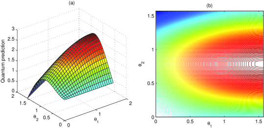
Figure 1: (color online). (a) Numerically calculated quantum prediction as a function of $\theta_{1}$ and $\theta_{2}$ for four-qubit GHZ state with $l=1$. (b) The contour lines of (a) show that the maximum occurs at $\theta_{1}=\pi/2$ and $\theta_{2}=\pi/4$.

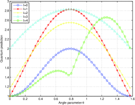
Figure 2: (color online). Numerical results of the relationship between quantum prediction and phase angle $\theta$ for the four-qubit GHZ state.

V Generalization and application

We now consider the generalized GHZ states with complex coefficients $\alpha$ and $\beta$. Let $\alpha\beta^{*}=|\alpha\beta^{*}|\text{e}^{-\text{i}\phi}$. Then, quantum correlation function can be rewritten as

$$E_{\textrm{QM}}(\phi_{1}^{k_{1}},\phi_{2}^{k_{2}},\cdots,\phi_{n}^{k_{n}}) = 2|\alpha\beta^{*}|\text{cos}(\phi+\phi_{1}^{k_{1}}+\phi_{2}^{k_{2}}+\cdots+\phi_{n}^{k_{n}}).$$ (29)

A similar calculation yields the quantum prediction

$$\sum_{j_{1},j_{2},\cdots,j_{n}=0,1}|q_{j_{1},j_{2},\cdots,j_{n}}| = |\alpha\beta^{*}|[(|\cos(\phi+\sum_{l=1,2,\cdots,n}\alpha_{l})|+|\sin(\phi+\sum_{l=1,2,\cdots,n}\alpha_{l})|)\prod_{l=1,2,\cdots,n}(|\cos\beta_{l}|+|\sin\beta_{l}|)$$ (30)

$$+(|\cos(\phi+\sum_{l=1,2,\cdots,n}\alpha_{l})|-|\sin(\phi+\sum_{l=1,2,\cdots,n}\alpha_{l})|)\prod_{l=1,2,\cdots,n}(|\cos\beta_{l}|-|\sin\beta_{l}|)].$$

When $\phi+\sum_{l=1,2,\cdots,n}\alpha_{l}$ and $\beta_{l}$ are $(2k+1)\pi/4$ $(k=0,\pm 1,\pm 2,\cdots)$, the maximum value $|\alpha\beta^{*}|2^{{(n+1)}/{2}}$ occurs. According to this result, the generalized Bell inequality will be violated conditioned on

$$|\alpha\beta^{*}|>2^{-\frac{n+1}{2}}.$$ (31)

As an important application, this provides a criterion for the violation of the generalized Bell inequality derived from the LHV theory; that is, under the present optimal measurement settings, for $|\alpha\beta^{*}|\leq 2^{-(n+1)/2}$ this inequality can not be violated. Especially, for real $\alpha$ and $\beta$, if we assume that $\alpha=\text{cos}\xi$ and $\beta=\text{sin}\xi$, then, consequently, for $\text{sin}2\xi\leq 2^{-(n-1)/2}$ the inequality can not be violated, which is consistent with the result in ZBLW2002 with an arbitrary odd $n$.

VI Discussion and summary

Having investigated the generalized Bell inequality and its maximal violation, we now discuss the possible experimental realization using optical quantum technologies DDI2006 ; Kok2007 ; Pan2012 . One aspect of this framework is the preparation of multiphoton entangled states. With linear optics and multiphoton interferometry, more recently, Pan et al. Pan-8-photon-GHZ-2012 ; Pan-10-photon-GHZ-2016 successively reported two schemes of observing eight-photon and ten-photon entanglement in experiment. By combining pairs of photons emitting from the parametric down-conversion processes SPDC1970 ; PDC1995 , eight-photon or ten-photon GHZ state can be engineered step by step. So, with currently available techniques, here one may produce the generalized GHZ state by considering a tunable angle parameter, which is settled by the orientation of a wave plate WSKPGW2008 ; LL-NJP2009 ; DHYG2017-4-photon . Another way of preparing multiphoton entangled states is to utilize cross-Kerr nonlinearities Imoto1985 ; SI1996 ; LI2000 ; NM2004 ; RV2005 ; Barrett2005 ; MNBS2005 ; Kok2008 ; HDYG2015OE ; HDYG2016SR . For example, we may consider an entangler of multiphoton GHZ states proposed by Ding et al. DYG2014 . By resetting an input state $(\alpha|H\rangle_{1}+\beta|V\rangle_{1})\otimes(|H\rangle_{2}+|V\rangle_{2})\otimes\cdots\otimes(|H\rangle_{n}+|V\rangle_{n})/2^{(n-1)/2}$, after the homodyne measurement on the probe beam the entangler is capable of preparing an $n$-photon generalized GHZ state. The other aspect of the present architecture is concerned with performing polarization analysis. Similar to the four-photon entanglement experiment EGBKZW2003 ; GBEKW2003 ; BEKGWGHBLS2004 ; XLG2006 , polarization analysis in various bases can be performed in each of the $n$ outputs via quarter- and half-wave plates in front of polarizing beam splitters. Taking the settings (27) (with $l=1$, $\theta_{1}=\pi/2$ and $\theta_{2}=\pi/4$) for example, the observer at site 1 switches analysis angle between 0 and $\pi/2$, and the other observers at sites $2,3,\cdots,n$ switch analysis angles between $\pm\pi/4$. When the $n$ photons are detected by single photon avalanche detectors, an $n$-fold coincidence detection can be registered. With these registrations one can investigate the violation of the generalized Bell inequality.

In summary, we have shown a method to deal with quantum nonlocality for $n$-qubit systems. Calculating the correlation function as an $n$-index tensor leads to a generalized Bell inequality. In this architecture, for an arbitrary $n$-qubit generalized GHZ state, under a set of experimental settings with various angle parameters, we have obtained the exact relationship between the amount of violation of the generalized Bell inequality and the variable angle parameters. By calculating the value of quantum prediction, as a result, we find a set of optimal measurement settings. Furthermore, as an example, we have shown a simplified description of $n$-qubit system involving two angle parameters. The main result is that when $l$ is odd there exists a set of optimal measurement settings, $\theta_{1}=\pi/2$ and $\theta_{2}=\pi/4$, and otherwise it does not exist. Finally, we calculate the quantum prediction for the generalized GHZ state with complex coefficients $\alpha$ and $\beta$. With the modified optimal measurement settings, an important criterion for the violation of the generalized Bell inequality have been demonstrated. Indeed, it is an interesting and useful fact in experimental tests of multipartite Bell-type inequalities.

Appendix A

In order to compute the quantum prediction

$$\sum_{j_{1},j_{2},\cdots,j_{n}=0,1}|q_{j_{1},j_{2},\cdots,j_{n}}|=\frac{|\alpha\beta|}{2^{n-1}}\sum_{j_{1},j_{2},\cdots,j_{n}=0,1}|\sum_{k_{1},k_{2},\cdots,k_{n}=0,1}(-1)^{\textbf{k}\centerdot\textbf{j}}\text{Re}[\text{e}^{-\text{i}(\phi_{1}^{k_{1}}+\phi_{2}^{k_{2}}+\cdots+\phi_{n}^{k_{n}})}]|,$$ (32)

we first let

$$A(\textbf{j})=\sum_{k_{1},k_{2},\cdots,k_{n}=0,1}(-1)^{\textbf{k}{}\centerdot\textbf{j}}\text{e}^{-\text{i}(\phi_{1}^{k_{1}}+\phi_{2}^{k_{2}}+\cdots+\phi_{n}^{k_{n}})}.$$ (33)

A simple calculation shows that

$$A(\textbf{j}) = \sum_{k_{1},k_{2},\cdots,k_{n}=0,1}(-1)^{k_{1}j_{1}}\text{e}^{-\text{i}\phi_{1}^{k_{1}}}(-1)^{k_{2}j_{2}}\text{e}^{-\text{i}\phi_{2}^{k_{2}}}\cdots(-1)^{k_{n}j_{n}}\text{e}^{-\text{i}\phi_{n}^{k_{n}}}$$ (34)

$$= \prod_{l=1,2,\cdots,n}[\text{e}^{-\text{i}\phi_{l}^{0}}+(-1)^{j_{l}}\text{e}^{-\text{i}\phi_{l}^{1}}]$$

$$= \prod_{l=1,2,\cdots,n}\text{e}^{-\text{i}\frac{(\phi_{l}^{1}+\phi_{l}^{0})}{2}}[\text{e}^{\text{i}\frac{(\phi_{l}^{1}-\phi_{l}^{0})}{2}}+(-1)^{j_{l}}\text{e}^{-\text{i}\frac{(\phi_{l}^{1}-\phi_{l}^{0})}{2}}]$$

$$= \prod_{l=1,2,\cdots,n}\text{e}^{-\text{i}\frac{(\phi_{l}^{1}+\phi_{l}^{0})}{2}}2[\text{cos}\frac{(\phi_{l}^{1}-\phi_{l}^{0})}{2}]^{1-j_{l}}[\text{i}\text{sin}\frac{(\phi_{l}^{1}-\phi_{l}^{0})}{2}]^{j_{l}}.$$

It follows immediately the definition of $\alpha_{l}$, $\beta_{l}$ in Eq.(22) that

$$A(\textbf{j})=2^{n}\text{e}^{\text{i}\sum_{l=1,2,\cdots,n}(-\alpha_{l}+{\frac{\pi}{2}}j_{l})}\prod_{l=1,2,\cdots,n}[\text{cos}\beta_{l}]^{1-j_{l}}[\text{sin}\beta_{l}]^{j_{l}}.$$ (35)

Taking the real part of $A(\textbf{j})$, there is

$$\text{Re}[A(\textbf{j})]=2^{n}\text{cos}[\sum_{l=1,2,\cdots,n}(-\alpha_{l}+{\frac{\pi}{2}}j_{l})]\prod_{l=1,2,\cdots,n}[\text{cos}\beta_{l}]^{1-j_{l}}[\text{sin}\beta_{l}]^{j_{l}}.$$ (36)

By calculation, one derive

$$\sum_{\textbf{j}}|\text{Re}[A(\textbf{j})]|$$ (37)

$$= 2^{n}\sum_{\textbf{j}}|\text{cos}[\sum_{l=1,2,\cdots,n}(-\alpha_{l}+{\frac{\pi}{2}}j_{l})]|\prod_{l=1,2,\cdots,n}|\text{cos}\beta_{l}|^{1-j_{l}}|\text{sin}\beta_{l}|^{j_{l}}$$

$$= 2^{n}\sum_{\textbf{j}}|\cos(\sum_{l=1,2,\cdots,n}\alpha_{l})\cos(\frac{\pi}{2}\sum_{l=1,2,\cdots,n}j_{l})+\sin(\sum_{l=1,2,\cdots,n}\alpha_{l})\sin(\frac{\pi}{2}\sum_{l=1,2,\cdots,n}j_{l})|\prod_{l=1,2,\cdots,n}|\text{cos}\beta_{l}|^{1-j_{l}}|\text{sin}\beta_{l}|^{j_{l}}$$

$$= 2^{n}|\sin(\sum_{l=1,2,\cdots,n}\alpha_{l})|\sum_{\textbf{j},\sum_{l=1,2,\cdots,n}j_{l}=\text{odd}}\prod_{l=1,2,\cdots,n}|\text{cos}\beta_{l}|^{1-j_{l}}|\text{sin}\beta_{l}|^{j_{l}}$$

$$+2^{n}|\cos(\sum_{l=1,2,\cdots,n}\alpha_{l})|\sum_{\textbf{j},\sum_{l=1,2,\cdots,n}j_{l}=\text{even}}\prod_{l=1,2,\cdots,n}|\text{cos}\beta_{l}|^{1-j_{l}}|\text{sin}\beta_{l}|^{j_{l}},$$

where the following identities

$$\sum_{l=1,2,\cdots,n}j_{l}=\text{odd},~{}~{}~{}~{}~{}\sin(\frac{\pi}{2}\sum_{l=1,2,\cdots,n}j_{l})=\pm 1,~{}~{}~{}~{}~{}~{}\cos(\frac{\pi}{2}\sum_{l=1,2,\cdots,n}j_{l})=0,\\$$ (38)

$$\sum_{l=1,2,\cdots,n}j_{l}=\text{even},~{}~{}~{}~{}~{}\sin(\frac{\pi}{2}\sum_{l=1,2,\cdots,n}j_{l})=0,~{}~{}~{}~{}~{}~{}\cos(\frac{\pi}{2}\sum_{l=1,2,\cdots,n}j_{l})=\pm 1\\$$ (39)

are used in the last equality.

Then we obtain

$$\sum_{\textbf{j}}|\text{Re}[A(\textbf{j})]|$$ (40)

$$= 2^{n-1}(|\cos(\sum_{l=1,2,\cdots,n}\alpha_{l})|+|\sin(\sum_{l=1,2,\cdots,n}\alpha_{l})|)\prod_{l=1,2,\cdots,n}(|\cos\beta_{l}|+|\sin\beta_{l}|)$$

$$+2^{n-1}(|\cos(\sum_{l=1,2,\cdots,n}\alpha_{l})|-|\sin(\sum_{l=1,2,\cdots,n}\alpha_{l})|)\prod_{l=1,2,\cdots,n}(|\cos\beta_{l}|-|\sin\beta_{l}|).$$

Therefore, the quantum prediction is given by

$$\sum_{j_{1},j_{2},\cdots,j_{n}=0,1}|q_{j_{1},j_{2},\cdots,j_{n}}|$$ (41)

$$= |\alpha\beta|\{[|\cos(\sum_{l=1,2,\cdots,n}\alpha_{l})|+|\sin(\sum_{l=1,2,\cdots,n}\alpha_{l})|]\prod_{l=1,2,\cdots,n}(|\cos\beta_{l}|+|\sin\beta_{l}|)$$

$$+[|\cos(\sum_{l=1,2,\cdots,n}\alpha_{l})|-|\sin(\sum_{l=1,2,\cdots,n}\alpha_{l})|]\prod_{l=1,2,\cdots,n}(|\cos\beta_{l}|-|\sin\beta_{l}|)\},$$

as desired.

Appendix B

By the definition $\sum_{l=1,2,\cdots,n}\alpha_{l}=\beta_{0}$, the quantum prediction

$$\sum_{j_{1},j_{2},\cdots,j_{n}=0,1}|q_{j_{1},j_{2},\cdots,j_{n}}|=|\alpha\beta|\{\prod_{l=0,1,2,\cdots,n}(|\cos\beta_{l}|+|\sin\beta_{l}|)+\prod_{l=0,1,2,\cdots,n}(|\cos\beta_{l}|-|\sin\beta_{l}|)\}.$$

Obviously, the quantum prediction is the function of $n+1$ independent variables $\beta_{0},\beta_{1},\cdots,\beta_{n}\in[0,\pi]$ by virtue of the periodic nature of the absolute values of sine and cosine functions. Furthermore, one can divide each of variables $\beta_{0},\beta_{1},\cdots,\beta_{n}\in[0,\pi]$ into two sections $[0,{\pi}/{2}]$ and $[{\pi}/{2},\pi]$.

Note that for $\beta_{l}\in[0,{\pi}/{2}]$,

$$|\cos\beta_{l}|+|\sin\beta_{l}|=\sqrt{2}\sin(\beta_{l}+\frac{\pi}{4}),$$ (42)

$$|\cos\beta_{l}|-|\sin\beta_{l}|=\sqrt{2}\cos(\beta_{l}+\frac{\pi}{4}).$$ (43)

While for $\beta_{l}\in[{\pi}/{2},\pi]$,

$$|\cos\beta_{l}|+|\sin\beta_{l}|=\sqrt{2}\sin(\beta_{l}-\frac{\pi}{4})=\sqrt{2}\sin[(\beta_{l}-\pi/2)+\frac{\pi}{4}],$$ (44)

$$|\cos\beta_{l}|-|\sin\beta_{l}|=-\sqrt{2}\cos(\beta_{l}-\frac{\pi}{4})=-\sqrt{2}\cos[(\beta_{l}-\pi/2)+\frac{\pi}{4}].$$ (45)

We use $\beta_{l}^{0}$, $\beta_{l}^{1}$ to denote $\beta_{l}\in[0,{\pi}/{2}]$, $\beta_{l}\in[{\pi}/{2},\pi]$, respectively. Thus, the $n+1$ intervals $\beta_{l}$ in $[0,{\pi}]$, can be divided into $2^{n+1}$ sections with $\beta_{l}^{0}$ in $[0,{\pi}/2]$ and $\beta_{l}^{1}$ in $[{\pi}/2,\pi]$. Therefore, in the section where the number of $\beta_{l}^{0}$ in $[0,{\pi}/2]$ is $(n+1-m)$, while the number of $\beta_{l}^{1}$ in $[0,{\pi}/2]$ is $m$, the quantum prediction should be

$$\sum_{j_{1},j_{2},\cdots,j_{n}=0,1}|q_{j_{1},j_{2},\cdots,j_{n}}|$$ (46)

$$= |\alpha\beta|2^{\frac{n+1}{2}}\{\prod_{l=0}^{m-1}\sin[(\beta_{l}^{1}-\pi/2)+\frac{\pi}{4}]\prod_{l=m}^{n}\sin(\beta_{l}^{0}+\frac{\pi}{4})$$

$$+(-1)^{m}\prod_{l=0}^{m-1}\cos[(\beta_{l}^{1}-\pi/2)+\frac{\pi}{4}]\prod_{l=m}^{n}\cos(\beta_{l}^{0}+\frac{\pi}{4})\}.$$

Obviously, in this section Eq. (46) is equivalent to

$$\sum_{j_{1},j_{2},\cdots,j_{n}=0,1}|q_{j_{1},j_{2},\cdots,j_{n}}|=|\alpha\beta|2^{\frac{n+1}{2}}[\prod_{l=0}^{n}\sin(\delta_{l}+\frac{\pi}{4})+(-1)^{m}\prod_{l=0}^{n}\cos(\delta_{l}+\frac{\pi}{4})],~{}~{}~{}\delta_{l}\in[0,{\pi}/2].$$ (47)

Let

$$F=|\alpha\beta|2^{\frac{n+1}{2}}[\prod_{l=0}^{n}\sin(\delta_{l}+\frac{\pi}{4})+\prod_{l=0}^{n}\cos(\delta_{l}+\frac{\pi}{4})],~{}~{}~{}\delta_{l}\in[0,{\pi}/2];$$ (48)

$$G=|\alpha\beta|2^{\frac{n+1}{2}}[\prod_{l=0}^{n}\sin(\delta_{l}+\frac{\pi}{4})-\prod_{l=0}^{n}\cos(\delta_{l}+\frac{\pi}{4})],~{}~{}~{}\delta_{l}\in[0,{\pi}/2].$$ (49)

Then, maximum value of the quantum prediction

$$\textrm{max}\sum_{j_{1},j_{2},\cdots,j_{n}=0,1}|q_{j_{1},j_{2},\cdots,j_{n}}|=\textrm{max}\{\textrm{max}F,\textrm{max}G\}.$$ (50)

Solving sets of differential equations $\partial F/\partial\delta_{l}=0$ produces $\delta_{l}=\pi/4$, $l=0,1,2,\cdots,n$. With these values it is obvious that the $(n+1)\times(n+1)$ matrix $(\partial^{2}F/{\partial{\delta_{i}}{\partial\delta_{j}}})$ is negative. So we have

$$\textrm{max}F=|\alpha\beta|2^{\frac{n+1}{2}}.$$

Similarly, there is

$$\textrm{max}G=|\alpha\beta|2^{\frac{n+1}{2}},$$

while also occurs at $\delta_{l}=\pi/4$, $l=0,1,2,\cdots,n$, that means $\beta_{l}^{0}=\pi/4,\beta_{l}^{1}=\pi/4+\pi/2$.

Together with the periodicity condition, we arrive at the conclusion that the maximum value of the quantum prediction is

$$\textrm{max}\sum_{j_{1},j_{2},\cdots,j_{n}=0,1}|q_{j_{1},j_{2},\cdots,j_{n}}|=|\alpha\beta|2^{\frac{n+1}{2}},$$ (51)

which occurs at $\beta_{l}=(2k+1)\pi/4$, $k=0,\pm 1,\pm 2,\cdots,$ $l=0,1,2,\cdots,n$.

References

• (1) J. S. Bell, On the Einstein-Podolsy-Rosen paradox, Physics (Long Island City, N.Y.) 1, 195–200 (1964).
• (2) J. F. Clauser, M. A. Horne, A. Shimony, and R. A. Holt, Proposed experiment to test local hidden-variable theories, Phys. Rev. Lett. 23, 880–884 (1969).
• (3) N. D. Mermin, Extreme quantum entanglement in a superposition of macroscopically distinct states, Phys. Rev. Lett. 65, 1838–1840 (1990).
• (4) M. Ardehali, Bell inequalities with a magnitude of violation that grows exponentially with the number of particles, Phys. Rev. A 46, 5375–5378 (1992).
• (5) A. V. Belinskiĭ and D. N. Klyshko, Interference of light and Bell’s theorem, Phys. Usp. 36, 653–693 (1993).
• (6) R. F. Werner and M. M. Wolf, All-multipartite Bell-correlation inequalities for two dichotomic observables per site, Phys. Rev. A 64, 032112 (2001).
• (7) M. Żukowski and Č. Brukner, Bell’s theorem for general N-qubit states, Phys. Rev. Lett. 88, 210401 (2002).
• (8) C. F. Wu, Y. Yeo, L. C. Kwek, and C. H. Oh, Quantum nonlocality of four-qubit entangled states, Phys. Rev. A 75, 032332 (2007).
• (9) S. Ghose, N. Sinclair, S. Debnath, P. Rungta, and R. Stock, Tripartite entanglement versus tripartite nonlocality in three-qubit Greenberger-Horne-Zeilinger-class states, Phys. Rev. Lett. 102, 250404 (2009).
• (10) M. Li and S. M. Fei, Bell inequalities for multipartite qubit quantum systems and their maximal violation, Phys. Rev. A 86, 052119 (2012).
• (11) Y. C. Wu, M. Żukowski, J. L. Chen, and G. C. Guo, Compact Bell inequalities for multipartite experiments, Phys. Rev. A 88, 022126 (2013).
• (12) D. Ding, Y. Q. He, F. L. Yan, and T. Gao, Quantum nonlocality of generic family of four-qubit entangled pure states, Chin. Phys. B 24, 070301 (2015).
• (13) Y. Q. He, D. Ding, F. L. Yan, and T. Gao, Scalable Bell inequalities for multiqubit systems, Europhys. Lett. 111, 40001 (2015).
• (14) N. Gisin, Bell’s inequality holds for all non-product states, Phys. Lett. A 154, 201 (1991).
• (15) N. Gisin and A. Peres, Maximal violation of Bell’s inequality for arbitrarily large spin, Phys. Lett. A 162, 15 (1992).
• (16) J. L. Chen, C. F. Wu, L. C. Kwek, and C. H. Oh, Gisin’s theorem for three qubits, Phys. Rev. Lett. 93, 140407 (2004).
• (17) M. Żukowski, Č. Brukner, W. Laskowski, and M. Wieśniak, Do all pure entangled states violate Bell’s inequalities for correlation functions, Phys. Rev. Lett. 88, 210402 (2002).
• (18) N. Brunner, D. Cavalcanti, S. Pironio, V, Scarani, and S. Wehner, Bell nonlocality, Rev. Mod. Phys. 86, 419–478 (2014).
• (19) F. Dell’Anno, S. De Siena, and F. Illuminati, Multiphoton quantum optics and quantum state engineering, Phys. Rep. 428, 53–168 (2006).
• (20) P. Kok, W. J. Munro, K. Nemoto, T. C. Ralph, J. P. Dowling, and G. J. Milburn, Linear optical quantum computing with photonic qubits, Rev. Mod. Phys. 79, 135–174 (2007).
• (21) J. W. Pan, Z. B. Chen, C. Y. Lu, H. Weinfurter, A. Zeilinger, and M. Żukowski, Multiphoton entanglement and interferometry, Rev. Mod. Phys. 84, 777–838 (2012).
• (22) M. Lassen, V. Delaubert, J. Janousek, K. Wagner, H. A. Bachor, P. K. Lam, N. Treps, P. Buchhave, C. Fabre, and C. C. Harb, Tools for multimode quantum information: modulation, detection, and spatial quantum correlations, Phys. Rev. Lett. 98, 083602 (2007).
• (23) L. Aolita, R. Gallego, A. Acín, A. Chiuri, G. Vallone, P. Mataloni, and A. Cabello, Fully nonlocal quantum correlations, Phys. Rev. A 85, 032107 (2012).
• (24) S. Carlig and M. A. Macovei, Quantum correlations among optical and vibrational quanta, Phys. Rev. A 89, 053803 (2014).
• (25) J. L. Li, K. Du, and C. F. Qiao, Connection between measurement disturbance relation and multipartite quantum correlation, Phys. Rev. A 91, 012110 (2015).
• (26) A. Kumar, H. Nunley, and A. M. Marino, Observation of spatial quantum correlations in the macroscopic regime, Phys. Rev. A 95, 053849 (2017).
• (27) H. Weinfurter and M. Żukowski, Four-photon entanglement from down-conversion, Phys. Rev. A 64, 010102 (2001).
• (28) Y. Li and T. Kobayashi, Four-photon entanglement from two-crystal geometry, Phys. Rev. A 69, 020302 (2004); Y. Li and T. Kobayashi, Phys. Rev. A 72, 059905(E) (2005).
• (29) D. Ding, Y. Q. He, F. L. Yan, and T. Gao, On four-photon entanglement from parametric down-conversion process, Quantum Informatiom Processing 17, 243 (2018).
• (30) X. C. Yao, T. X. Wang, P. Xu, H. Lu, G. S. Pan, X. H. Bao, C. Z. Peng, C. Y. Lu, Y. A. Chen, and J. W. Pan, Observation of eight-photon entanglement, Nat. Photonics 6, 225–228 (2012).
• (31) X. L. Wang, L. K. Chen, W. Li, H. L. Huang, C. Liu, C. Chen, Y. H. Luo, Z. E. Su, D. Wu, Z. D. Li, H. Lu, Y. Hu, X. Jiang, C. Z. Peng, L. Li, N. L. Liu, Y. A. Chen, C. Y. Lu, and J. W. Pan, Experimental ten-photon entanglement, Phys. Rev. Lett. 117, 210502 (2016).
• (32) D. C. Burnham and D. L. Weinberg, Observation of simultaneity in parametric production of optical photon pairs, Phys. Rev. Lett. 25, 84–87 (1970).
• (33) P. G. Kwiat, K. Mattle, H. Weinfurter, A. Zeilinger, A. V. Sergienko, and Y. Shih, New high-intensity source of polarization-entangled photon pairs, Phys. Rev. Lett. 75, 4337–4341 (1995).
• (34) W. Wieczorek, C. Schmid, N. Kiesel, R. Pohlner, O. Gühne, and H. Weinfurter, Experimental observation of an entire family of four-photon entangled states, Phys. Rev. Lett. 101, 010503 (2008).
• (35) B. P. Lanyon and N. K. Langford, Experimentally generating and tuning robust entanglement between photonic qubits, New J. Phys. 11, 013008 (2009).
• (36) N. Imoto, H. A. Haus, and Y. Yamamoto, Quantum nondemolition measurement of the photon number via the optical Kerr effect, Phys. Rev. A 32, 2287–2292 (1985).
• (37) H. Schmidt and A. Imamoğlu, Giant Kerr nonlinearities obtained by electromagnetically induced transparency, Opt. Lett. 21, 1936–1938 (1996).
• (38) M. D. Lukin and A. Imamoğlu, Nonlinear optics and quantum entanglement of ultraslow single photons, Phys. Rev. Lett. 84, 1419–1422 (2000).
• (39) K. Nemoto and W. J. Munro, Nearly deterministic linear optical controlled-NOT gate, Phys. Rev. Lett. 93, 250502 (2004).
• (40) H. Rokhsari and K. J. Vahala, Observation of Kerr nonlinearity in microcavities at room temperature, Opt. Lett. 30, 427–429 (2005).
• (41) S. D. Barrett, P. Kok, K. Nemoto, R. G. Beausoleil, W. J. Munro, and T. P. Spiller, Symmetry analyzer for nondestructive Bell-state detection using weak nonlinearities, Phys. Rev. A 71, 060302 (2005).
• (42) W. J. Munro, K. Nemoto, R. G. Beausoleil, and T. P. Spiller, High-efficiency quantum-nondemolition single-photon-number-resolving detector, Phys. Rev. A 71, 033819 (2005).
• (43) P. Kok, Effects of self-phase-modulation on weak nonlinear optical quantum gates, Phys. Rev. A 77, 013808 (2008).
• (44) Y. Q. He, D. Ding, F. L. Yan, and T. Gao, Exploration of photon-number entangled states using weak nonlinearities, Opt. Express 23, 21671–21677 (2015).
• (45) Y. Q. He, D. Ding, F. L. Yan, and T. Gao, Exploration of multiphoton entangled states by using weak nonlinearities, Sci. Rep. 6, 19116 (2016).
• (46) D. Ding, F. L. Yan, and T. Gao, Entangler and analyzer for multiphoton Greenberger-Horne-Zeilinger states using weak nonlinearities, Sci. China-Phys. Mech. Astron. 57, 2098–2103 (2014).
• (47) M. Eibl, S. Gaertner, M. Bourennane, C. Kurtsiefer, M. Żukowski, and H. Weinfurter, Experimental observation of four-photon entanglement from parametric down-conversion, Phys. Rev. Lett. 90, 200403 (2003).
• (48) S. Gaertner, M. Bourennane, M. Eibl, C. Kurtsiefer, and H. Weinfurter, High-fidelity source of four-photon entanglement, Appl. Phys. B 77, 803-807 (2003).
• (49) M. Bourennane, M. Eibl, C. Kurtsiefer, S. Gaertner, H. Weinfurter, O. Gühne, P. Hyllus, D. Bruß, M. Lewenstein, and A. Sanpera, Experimental detection of multipartite entanglement using witness operators, Phys. Rev. Lett. 92, 087902 (2004).
• (50) J. S. Xu, C. F. Li, and G. C. Guo, Generation of a high-visibility four-photon entangled state and realization of a four-party quantum communication complexity scenario, Phys. Rev. A 74, 052311 (2006).