Discovering Influential Factors in Variational Autoencoder

Abstract

In the field of machine learning, it is still a critical issue to identify and supervise the learned representation without manually intervening or intuition assistance to extract useful knowledge or serve for the downstream tasks. In this work, we focus on supervising the influential factors extracted by the variational autoencoder(VAE). The VAE is proposed to learn independent low dimension representation while facing the problem that sometimes pre-set factors are ignored. We argue that the mutual information of the input and each learned factor of the representation plays a necessary indicator of discovering the influential factors. We find the VAE objective inclines to induce mutual information sparsity in factor dimension over the data intrinsic dimension and results in some non-influential factors whose function on data reconstruction could be ignored. We show mutual information also influences the lower bound of VAE’s reconstruction error and downstream classification task. To make such indicator applicable, we design an algorithm for calculating the mutual information for VAE and prove its consistency. Experimental results on MNIST, CelebA and DEAP datasets show that mutual information can help determine influential factors, of which some are interpretable and can be used to further generation and classification tasks, and help discover the variant that connects with emotion on DEAP dataset.

Introduction

Learning efficient low dimension representation of data is important in machine learning and related applications. Efficient and intrinsic low dimension representation is helpful to exploit the underlying knowledge of data and serves for downstream tasks including generation, classification and association. Early linear dimension reduction (Principle Component Analysis) has been widely used in primary data analysis and its variant has been applied in face identification (Yang et al. (2004)) and classical linear independent representation (Independent Component Analysis (Hyvärinen, Karhunen, and Oja (2004)) have been used in blind source separation (Jung et al. (2000)) and EEG signal processing (Makeig et al. (1996)). Nonlinear dimension reduction (e.g. Autoencoder (Goodfellow, Bengio, and Courville (2016))) begins to further learn abstract representation and has been used in semantic hashing (Salakhutdinov and Hinton (2009) and many other tasks. Recently, a new technique, called variational autoencoder (Kingma and Welling (2013); Rezende, Mohamed, and Wierstra (2014)) has attracted much attention of researchers, due to its capability in extracting nonlinear independent representation. The method can further model causal relationship, represent disentangled visual variants (Mathieu et al. (2016)) and interpretable time series variants (Hsu, Zhang, and Glass (2017)) and this method can serve for generating signals with abundant diversities in a “factor-controllable” way (Suzuki, Nakayama, and Matsuo (2016); Higgins et al. (2017b)). The related techniques enable the knowledge transferring through shared factors among different tasks (Higgins et al. (2017a)).

However, the usage of VAE on extracting factors are unclear and we lack efficient methodologies to quantify the influence of each learned factor on data representation. In application, sometimes some pre-set factors remain unused (Goodfellow, Bengio, and Courville (2016)), and the relation between the learned factors and original data has to be discovered by manually intervention (visual or aural observation). This leads to the waste on extra factors and hinders the factor selection for the subsequent tasks such as generating meaningful image/audio. Besides, some classical influence determination methods including estimating the variance of each factor lose its utility on the VAE. Therefore, identifying and monitoring the influential factor of VAE becomes a critical issue along this line of research.

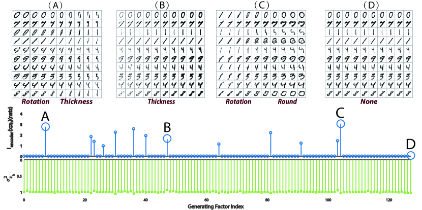
Figure 1: Estimated $I(\mathbf{x};{z_{\mathbf{enc}}}_{h})$ determines the influential factors; $I(\mathbf{x};{z_{\mathbf{enc}}}_{h})$, $\sigma^{2}_{z_{h}}$ and qualitatively influential factor traversals of $\beta(=10)$-VAE on MNIST. The top pulse subgraph: $I(\mathbf{x};{z_{\mathbf{enc}}}_{h})$ of each factor. The bottom reverse pulse subgraph: the estimated variance $\sigma^{2}_{z_{h}}$ of each factor. The A,B,C montages: influential factor traversals corresponding to factor A,B,C noted in the pulse graph and the whole influential factor traversals are listed in Fig.(7) in Appendix B. The montages D is the traversal of ignored factors with little estimated mutual information. According to the four montages, the variance can’t determine the influential factors as mutual information indicator does.

In order to efficiently determine and supervise the learned factors, this paper has made the following efforts.

• We first adopt mutual information as the quantitative indicator of assessing the influence of each factor on data representation in the VAE model. Besides, in order to analyze the rationality of this indicator, we theoretically prove that how mutual information influence the lower bound of VAE’s reconstruction error and subsequent classification task.

• We propose an estimation algorithms to calculate the mutual information for all the factors of VAE, and then we prove its consistency.

• We substantiate the effectiveness of the proposed indicator by experiments on MNIST (Lécun et al. (1998)), CelebA (Liu et al. (2015)) and DEAP (Koelstra et al. (2012)). Especially, some discovered factors by the proposed indicator are found meaningful and interpretable for data representation and other left ones are generally ignorable for the task. The capability of the selected factors on generalization and classification tasks are also verified.

This paper is organized as the following. We introduce the VAE model for generation and classification in Section 2. We argue the necessity of mutual information as a indicator in Section 3. Specifically, we introduce the mutual information of input data and factors, analyze the cause through the perspective of mutual information and data intrinsic dimension, discuss the relationship of mutual information and recover as well as the classification and propose the estimator and prove its consistency. We review the related work on supervising the factors of VAE in Section 4. The experiments are in Section 5.

VAE model

VAE (Kingma and Welling (2013), Rezende, Mohamed, and Wierstra (2014)) is a scalable unsupervised representation learning model (Higgins et al. (2016)): VAE assumes that input $\mathbf{x}$ is generated by several independent Gaussian random variables $\mathbf{z}$, that is $p_{\mathbf{dec}}(\mathbf{z})=\mathcal{N}(\mathbf{z}|\textbf{0},I_{H})$. Since Gaussian distribution can be continuously and reversibly mapping to many other distributions, the theoretical analysis on it might be also instructive for other continuous-latent VAEs. The generating/decoding process is modeled as $p_{\mathbf{dec}}(\mathbf{x}|\mathbf{z})$ and the inference/encoding process $q_{\mathbf{enc}}(\mathbf{z}|\mathbf{x})=\mathcal{N}(\mathbf{z}|$$\mu$$(\mathbf{x}),diag(\sigma_{1}(\mathbf{x}),\cdots,\sigma_{H}(\mathbf{x})))$ is treated as the approximate posterior distribution. Note that it yields that $q_{\mathbf{enc}}(\mathbf{z}|\mathbf{x})=q_{\mathbf{enc}}(z_{1}|\mathbf{x})\cdots q_{\mathbf{enc}}(z_{H}|\mathbf{x})$. We assume both of them are parameterized by the neural network with parameter $\mathbf{enc}$ and $\mathbf{dec}$.

Factor: Let $\mathbf{z}_{\mathbf{enc}}$ denote random variables determined by $q_{\mathbf{enc}}(\mathbf{z})=\int q_{\mathbf{enc}}(\mathbf{z}|\mathbf{x})p_{data}(\mathbf{x})d\mathbf{x}$ and a factor in the latter literature refers to a dimension of $\mathbf{z}_{\mathbf{enc}}$.

Generation

In VAE setting, the approximate inference method is applied to maximizing the variational lower bound of $\log p_{\mathbf{dec}}(\mathbf{x})=\log\int p_{\mathbf{dec}}(\mathbf{x}|\mathbf{z})p_{\mathbf{dec}}(\mathbf{z})d\mathbf{z}$,

$$\mathcal{L}_{rec} = \mathop{{\mathbb{E}}}\limits\limits_{\mathbf{z}\sim q_{\mathbf{enc}}(\mathbf{z}|\mathbf{x})}\log p_{\mathbf{dec}}(\mathbf{z}|\mathbf{x})-D_{KL}(q_{\mathbf{enc}}(\mathbf{z}|\mathbf{x})||p_{\mathbf{dec}}(\mathbf{z}))$$ (1)

$$\leq \log p_{\mathbf{dec}}(\mathbf{x}),$$

with the equality holds iff

$$D_{KL}(q_{\mathbf{enc}}(\mathbf{z}|\mathbf{x})||p_{\mathbf{dec}}(\mathbf{z}|\mathbf{x}))=0.$$ (2)

In order to limit the information channel capacity (Higgins et al. (2016)), $\beta$-VAE introduces $\beta>1$ to the second term of the objective,

$$\mathcal{L}_{rec-\beta} = \mathop{{\mathbb{E}}}\limits\limits_{\mathbf{z}\sim q_{\mathbf{enc}}(\mathbf{z}|\mathbf{x})}\log p_{\mathbf{dec}}(\mathbf{z}|\mathbf{x})-$$ (3)

$$\ \ \ \ \ \ \ \ \ \ \beta D_{KL}(q_{\mathbf{enc}}(\mathbf{z}|\mathbf{x})||p_{\mathbf{dec}}(\mathbf{z}))$$

$$< \log p_{\mathbf{dec}}(\mathbf{x}).$$

After training the objective, by sampling from the $p_{\mathbf{dec}}(\mathbf{z})=\mathcal{N}(\mathbf{z}|\textbf{0},I_{H})$ or setting $\mathbf{z}$ with purpose, the learned $p_{\mathbf{dec}}(\mathbf{x}|\mathbf{z})$ can generate new samples.

Classification

The $q_{\mathbf{enc}}(\mathbf{z}|\mathbf{x})$ can further support latter tasks such as classification. Let $p_{\mathbf{pre}}(\mathbf{y}|\mathbf{z})$ denote the predicting process, and the classification objective is the following,

$$\mathcal{L}_{pre}=\mathop{{\mathbb{E}}}\limits\limits_{\mathbf{z}\sim q_{\mathbf{enc}}(\mathbf{z}|\mathbf{x})}\log p_{\mathbf{pre}}(\mathbf{y}|\mathbf{z}).$$ (4)

In real implementation the above objectives should further take expectation on the data distribution. However, sometimes only part factors are manually found useful for the generation (Goodfellow, Bengio, and Courville (2016)), and the factor which is irrelevant to $\mathbf{x}$ can not support classification either. Therefore, some approaches to automatically find the influential factor beneficial to the latter tasks are demanded.

Mutual Information as A Necessary Indicator

By exploring why factors are ignored, we argue that mutual information is a necessary indicator to find the influential factor.

Ignored Factor Analysis

Low Intrinsic Dimension of Data

One aim of the VAE is to learn the data intrinsic factors but intrinsic dimension keeps the same under the continuous reversible mapping suggested by Theorem 1.

Theorem 1 (Information Conservation).

Suppose that $\mathbf{z}=(z_{1},\cdots,z_{H})$ and $\mathbf{y}=(y_{1},\cdots,y_{P})$ are sets of $H$ and $P$ ($H\neq P$) independent unit Gaussian random variables, respectively, then these two sets of random variables can not be the generating factor of each other. That is, there are no continuous functions $f:\mathbb{R}^{H}\rightarrow\mathbb{R}^{P}$ and $g:\mathbb{R}^{P}\rightarrow\mathbb{R}^{H}$ such that

$$\mathbf{z}=g(\mathbf{y})\quad and\quad\mathbf{y}=f(\mathbf{z}).$$

Proof is listed in Appendix A. Suppose the oracle data, denoted by random variable $\mathbf{x}$, is generated by $\mathbf{y}$ (with $P$ independent unit Gaussian random variables) with a homeomorphism mapping $\mathbf{x}=\phi(\mathbf{y})$. Factors $\mathbf{z}$ (with $H$ independent unit Gaussian random variables) generates the $\mathbf{x}$ with a homeomorphism mapping $\mathbf{x}=\psi(\mathbf{z})$. It yields $\mathbf{z}=\psi^{-1}\circ\phi(\mathbf{y})$ and $\mathbf{y}=\phi^{-1}\circ\psi(\mathbf{z})$. Then according to the information conservation theorem, it must hold that $H=P$.

For example, 10 Gaussian factors and 128 Gaussian factors can not generate each other. Analogically, if the data are generated by 10 intrinsic Gaussian factors, it intuitively would not be inferred to 128 Gaussian factors by VAE and some factors would be independent with data although we may pre-set in this way.

Mutual Information Reflexes the Absolute Statistic Dependence

In order to quantify the dependence and estimate which factor influences the generating process or has no effect at all, the mutual information of $\mathbf{z}_{\mathbf{enc}}$ and $\mathbf{x}$, $I(\mathbf{x};{z_{\mathbf{enc}}}_{h})$ can be taken as a rational indicator(Peng, Long, and Ding (2005)) . That is,

$$I(\mathbf{x};{z_{\mathbf{enc}}}_{h})=\mathop{{\mathbb{E}}}\limits_{\mathbf{x}\sim p_{data}(\mathbf{x})}D_{KL}(q_{\mathbf{enc}}(z_{h}|\mathbf{x})||q_{\mathbf{enc}}(z_{h})).$$ (5)

The mutual information can reflect the absolute statistic dependence: $I(\mathbf{x};{z_{\mathbf{enc}}}_{h})=0$ if and only if $\mathbf{x}$ and ${z_{\mathbf{enc}}}_{h}$ are independent. The larger $I(\mathbf{x};{z_{\mathbf{enc}}}_{h})$ is, the more information $z_{h}$ conveys regarding $\mathbf{x}$, and the more influential factor it should be to represent the data.

Sparsity in Mutual Information

Actually, mutual information is implicitly involved in the VAE objective. The following theorem further suggests the VAE objective induces the sparsity in mutual information. It then explains why factors are ignored from the perspective of mutual information.

Theorem 2 (Objective Decomposition).

If $q_{\mathbf{enc}}(\mathbf{z}|\mathbf{x})\ll p_{\mathbf{dec}}(\mathbf{z})$, for any $\mathbf{x}$, $q_{\mathbf{enc}}(\mathbf{z}|\mathbf{x})=q_{\mathbf{enc}}(z_{1}|\mathbf{x})\cdots q_{\mathbf{enc}}(z_{H}|\mathbf{x})$ and $p_{\mathbf{dec}}(\mathbf{z})=\mathcal{N}(\mathbf{z}|\textbf{0},I_{H})$ then it yields the following decomposition:

• $L_{1}$ norm expression of the KL-divergence term in VAE:

  $$\mathop{{\mathbb{E}}}\limits_{\mathbf{x}\sim p_{data}(\mathbf{x})}D_{KL}(q_{\mathbf{enc}}(\mathbf{z}|\mathbf{x})||p_{\mathbf{dec}}(\mathbf{z}))$$ (6)

  $$= \sum_{h=1}^{H}\mathop{{\mathbb{E}}}\limits_{\mathbf{x}\sim p_{data}(\mathbf{x})}D_{KL}(q_{\mathbf{enc}}(z_{h}|\mathbf{x})||p_{\mathbf{dec}}(z_{h}))$$

  $$= \|(\mathop{{\mathbb{E}}}\limits_{\mathbf{x}\sim p_{data}(\mathbf{x})}D_{KL}(q_{\mathbf{enc}}(z_{1}|\mathbf{x})||p_{\mathbf{dec}}(z_{1})),$$

  $$\mathop{{\mathbb{E}}}\limits_{\mathbf{x}\sim p_{data}(\mathbf{x})}D_{KL}(q_{\mathbf{enc}}(z_{2}|\mathbf{x})||p_{\mathbf{dec}}(z_{2})),\cdots,$$

  $$\mathop{{\mathbb{E}}}\limits_{\mathbf{x}\sim p_{data}(\mathbf{x})}D_{KL}(q_{\mathbf{enc}}(z_{h}|\mathbf{x})||p_{\mathbf{dec}}(z_{h})))\|_{1}.$$

• Further decomposition of an entity in the $L_{1}$ norm expression:

  $$\mathop{{\mathbb{E}}}\limits_{\mathbf{x}\sim p_{data}(\mathbf{x})}D_{KL}(q_{\mathbf{enc}}(z_{h}|\mathbf{x})||p_{\mathbf{dec}}(z_{h}))$$ (7)

  $$= I(\mathbf{x};{z_{\mathbf{enc}}}_{h})+D_{KL}(q_{\mathbf{enc}}(z_{h})||p_{\mathbf{dec}}(z_{h})).$$

Proof is given in Appendix A. The theorem demonstrates that the expectation of the second term in variation lower bound in Eq. (1) can be represented in the form of $L_{1}$ norm which inclines to induce the sparsity of $I(\mathbf{x};{z_{\mathbf{enc}}}_{h})$ and $D_{KL}(q_{\mathbf{enc}}(z_{h})||p_{\mathbf{dec}}(z_{h}))$ together in $h$, clipping down the non-intrinsic factor dimension to some extent. The sparsity of Expectation $\mathop{{\mathbb{E}}}\limits_{\mathbf{x}\sim p_{data}(\mathbf{x})}D_{KL}(q_{\mathbf{enc}}(z_{h}|\mathbf{x})||p_{\mathbf{dec}}(z_{h}))$ actually leads to sparsity of both its summarization terms $I(\mathbf{x};{z_{\mathbf{enc}}}_{h})$ and $D_{KL}(q_{\mathbf{enc}}(z_{h})||p_{\mathbf{dec}}(z_{h}))$ together in $h$, since both of them are non-negative. For any zero value summarization, both of its elements should also be zero. Thus this regularization term inclines to intrinsically conduct sparsity of mutual information $I(\mathbf{x};{z_{\mathbf{enc}}}_{h})$, which have been comprehensively substantiated by all our experiments, as can be easily seen in Fig.(1) and Fig.(2).

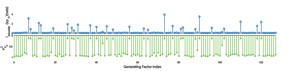
(A) $I(\mathbf{x};{z_{\mathbf{enc}}}_{h})$, $\sigma^{2}_{z_{h}}$ plot of $\beta(=40)$-VAE on CelebA.

(B) $I(\mathbf{x};{z_{\mathbf{enc}}}_{h})$, $\sigma^{2}_{z_{h}}$ plot of $\beta(=6)$-VAE on DEAP.

Figure 2: Mutual information sparsity occurs on CelebA and DEAP.

Therefore VAE objective inclines to induce mutual information sparsity in factor dimension over the data intrinsic dimension and the factor ignored phenomenon occurs. On the one hand, with this KL divergence regularization, even when the number of latent factors are set large, unlike auto-encoder, the over-fitting issue still tends not to occur. On the other hand, this helps us get influential factors to represent the variants of data, and facilitate an efficient generalization of data by varying these useful factors while neglecting others.

By the way, the following theorem suggests the condition that we can use $I(\mathbf{x};z_{h})$ to estimate the whole mutual information.

Theorem 3 (Mutual Information Separation).

Let $z_{1},\cdots,z_{h}$ be independent unit Gaussian distribution, and $z_{1},z_{2},\cdots,z_{h}$ be conditional independent given $\mathbf{x}$. Then

$$I(\mathbf{x};z_{1},\cdots,z_{h}) = \sum_{h=1}^{H}I(\mathbf{x};z_{h})$$ (8)

$$= \|(I(\mathbf{x};z_{1}),I(\mathbf{x};z_{2}),\cdots,I(\mathbf{x};z_{h}))\|_{1}.$$

Proof is presented in Appendix A. This theorem suggests that if the learnt $q_{\mathbf{enc}}(\mathbf{z})$ can factorize and the $q_{\mathbf{enc}}(\mathbf{z}|\mathbf{x})$ can factorize, then we could use the sum of $I(\mathbf{x};{z_{\mathbf{enc}}}_{h})$ to direct estimate the whole mutual information.

Reconstruction and Classification Theoretical Supports

According to Cover and Thomas (2012), the mutual information can also provide a lower bound for the best mean recover error.

Theorem 4.

Suppose $\mathbf{x}$ is with differential entropy $H(\mathbf{x})$, then let $\hat{\mathbf{x}}(\mathbf{z}_{\mathbf{enc}})$ be an estimation of $\mathbf{x}$, and give side information $\mathbf{z}_{\mathbf{enc}}$, and then it holds that

$$\mathop{{\mathbb{E}}}\limits(\mathbf{x}-\hat{\mathbf{x}}(\mathbf{z}_{\mathbf{enc}}))^{2}\geq\frac{1}{2\pi e}e^{2(H(\mathbf{x})-I(\mathbf{x};\mathbf{z}_{\mathbf{enc}}))}.$$ (9)

Therefore, if we set $p_{\mathbf{dec}}(\mathbf{x}|\mathbf{z})=\mathcal{N}(\mathbf{x}|\mathbf{dec}(\mathbf{z}),\sigma)$, then $\mathbf{x}_{rec}=\mathbf{dec}(\mathbf{z}_{\mathbf{enc}})$ has $\frac{1}{2\pi e}e^{2(H(\mathbf{x})-I(\mathbf{x};\mathbf{z}_{\mathbf{enc}}))}$ as the lower bound for recover. Let us only use a major set of factors $\mathbf{z}_{major}$: $\mathbf{x}_{recc}=\mathbf{dec}(\mathbf{z}_{major},\mathbf{0})$. With the assumption that $q_{\mathbf{enc}}(\mathbf{z})$ can factorize, it yields the separation of mutual information $I(\mathbf{x};\mathbf{z}_{\mathbf{enc}})=I(\mathbf{x};\mathbf{z}_{minor})+I(\mathbf{x};\mathbf{z}_{major})$. It yields the following bound,

$$\mathop{{\mathbb{E}}}\limits(\mathbf{x}-\mathbf{x}_{recc})^{2}$$ (10)

$$\geq \frac{1}{2\pi e}e^{2(H(\mathbf{x})-I(\mathbf{x};\mathbf{z}_{major}))}$$

$$\geq \frac{1}{2\pi e}e^{2(H(\mathbf{x})-I(\mathbf{x};\mathbf{z}_{major}))}e^{-2I(\mathbf{x};\mathbf{z}_{minor})}.$$

The theorem implies that the mutual information carried by the selecting factors directly influences on the lower bound of the best recover and we may select some top influential factors carrying the most information to represent and generate the data with less reconstruction distortion.

We further provide some theoretical supports for the proposed mutual information as the factor indicator in classification.

Suppose that Markov chain condition, $\mathbf{y}\to\mathbf{x}\to\mathbf{z}_{\mathbf{enc}}\to\mathbf{y}_{pre}$, holds, according to the Fano’s inequality (Cover and Thomas (2012)) and the information processing inequality the mutual information also correlates with the classification error.

Theorem 5 (Fano’s inequality).

For any estimation $\hat{\mathbf{y}}$ such that $\mathbf{y}\to\mathbf{z}_{\mathbf{enc}}\to\mathbf{y}_{pre}$, with $P_{e}=Pr(\hat{\mathbf{y}}\neq\mathbf{y})$, we have

$$H(P_{e})+P_{e}log|\mathcal{Y}|\geq H(\mathbf{y})-I(\mathbf{y};\mathbf{z}_{\mathbf{enc}})\geq H(\mathbf{y})-I(\mathbf{x};{\mathbf{z}_{\mathbf{enc}}}).$$ (11)

This inequality can be weakened to

$$1+P_{e}log|\mathcal{Y}|\geq H(\mathbf{y})-I(\mathbf{y};\mathbf{z}_{\mathbf{enc}})\geq H(\mathbf{y})-I(\mathbf{x};{\mathbf{z}_{\mathbf{enc}}}).$$ (12)

or

$$P_{e}\geq\frac{H(\mathbf{y})-I(\mathbf{y};\mathbf{z}_{\mathbf{enc}})-1}{log|\mathcal{Y}|}\geq\frac{H(\mathbf{y})-I(\mathbf{x};{\mathbf{z}_{\mathbf{enc}}})-1}{log|\mathcal{Y}|}.$$ (13)

Note that according to information processing inequality $I(\mathbf{x};{z_{\mathbf{enc}}}_{h})\geq I(\mathbf{y};{z_{\mathbf{enc}}}_{h})$. If $I(\mathbf{x};{z_{\mathbf{enc}}}_{h})=0\Rightarrow I(\mathbf{y};{z_{\mathbf{enc}}}_{h})=0$, the $h$ factor will not influence the prediction. With the assumption that $q_{\mathbf{enc}}(\mathbf{z})$ can factorize, the theorem suggests the mutual information carried by the selecting factors directly influences the lower bound of the classification error and therefore we can remove minor factors according to the mutual information $I(\mathbf{x};{z_{\mathbf{enc}}}_{h})$ without significantly lifting the lower bound of the prediction error.

Algorithms to Quantitatively Calculate the Proposed indicators

In order to calculate $I(\mathbf{x};\mathbf{z}_{\mathbf{enc}})$ in practice, we assume that $q^{*}(\mathbf{z})=\mathcal{N}(\mathbf{z}|\textbf{0},diag(\sigma^{*}_{1},\cdots,\sigma^{*}_{H}))$ is a factorized zero mean Gaussian estimation for $q_{\mathbf{enc}}(\mathbf{z})$.

We can then list the indicators to be estimated as:

Definition 1 (Estimation for $I(\mathbf{x};\mathbf{z}_{\mathbf{enc}})$: the information conveyed by whole factors).

$$I_{est}(\mathbf{x};\mathbf{z}_{\mathbf{enc}})_{M}=\frac{1}{M}\sum_{m=1}^{M}D_{KL}(q_{\mathbf{enc}}(\mathbf{z}|\mathbf{x}^{m})||q^{*}(\mathbf{z})).$$ (14)

This estimation uses $M$ sample according to the empirical form of Corollary 2.

Definition 2 (Estimation for $I(\mathbf{x};{z_{\mathbf{enc}}}_{h})$: the information conveyed by a factor).

$$I_{est}(\mathbf{x};{z_{\mathbf{enc}}}_{h})_{M}=\frac{1}{M}\sum_{m=1}^{M}D_{KL}(q_{\mathbf{enc}}({z_{\mathbf{enc}}}_{h}|\mathbf{x}^{m})||q^{*}({z_{\mathbf{enc}}}_{h})).$$ (15)

This indicator quantifies mutual information of a specific factor and input data.

Note that the above indicators need the value of $q^{*}(\mathbf{z})$, and thus we need to design algorithms to calculate this term. Based on Theorem 2 through the minimization equivalence, we know that

$$\min_{q}\mathop{{\mathbb{E}}}\limits_{\mathbf{x}\sim p_{data}(\mathbf{x})}D_{KL}(q_{\mathbf{enc}}(\mathbf{z}|\mathbf{x})||q(\mathbf{z}))$$

$$\Leftrightarrow\min_{q}D_{KL}(q_{\mathbf{enc}}(\mathbf{z})||q(\mathbf{z}))d\mathbf{z},$$ (16)

and then we can prove the following result:

Corollary 1.

if $q_{\mathbf{enc}}(\mathbf{z}|\mathbf{x})\ll q^{*}(\mathbf{z})$ then

$$\mathop{{\mathbb{E}}}\limits_{\mathbf{x}\sim p_{data}(\mathbf{x})}D_{KL}(q_{\mathbf{enc}}(\mathbf{z}|\mathbf{x})||q^{*}(\mathbf{z}))$$ (17)

$$= I(\mathbf{x};\mathbf{z}_{\mathbf{enc}})+D_{KL}(q_{\mathbf{enc}}(\mathbf{z})||q^{*}(\mathbf{z})).$$

The proof of Corollary 1 is the same as that of Theorem 2. This corollary suggests that the estimation defined in Definition 1 provides another upper bound for the capacity of the encoder network. Empirically, this estimation is a much tighter estimation than the second term of the Objective (1).

$q^{*}(\mathbf{z})$ can then be obtained by solving the following optimization problem:

$$q^{*}(\mathbf{z})=\arg\min_{q}\frac{1}{M}\sum_{m=1}^{M}D_{KL}(q_{\mathbf{enc}}(\mathbf{z}|\mathbf{x}^{m})||q(\mathbf{z})).$$ (18)

The above procedure is summarized and presented in Algorithm 1 to calculate the proposed indicators.

Algorithm 1 Mutual Information Estimation

1:  Input: Sampled Data $\{\mathbf{x}^{m}\}_{m=1}^{M}$,Encoder Network $q_{\mathbf{enc}}(\mathbf{z}|\mathbf{x})=\mathcal{N}(\mathbf{z}|$$\mathbf{\mu}$$(\mathbf{x}),diag(\sigma_{1}(\mathbf{x}),\cdots,\sigma_{H}(\mathbf{x})))$

2:  Obtain: $q^{*}(\mathbf{z})=\arg\min_{q}\frac{1}{M}\sum_{m=1}^{M}D_{KL}(q_{\mathbf{enc}}(\mathbf{z}|\mathbf{x}^{m})||q(\mathbf{z})).$

3:  Calculate: $I_{est}(\mathbf{x};{z_{\mathbf{enc}}}_{h})_{M}=\frac{1}{M}\sum_{m=1}^{M}D_{KL}(q_{\mathbf{enc}}({z_{\mathbf{enc}}}_{h}|\mathbf{x}^{m})||q^{*}({z_{\mathbf{enc}}}_{h}))$

4:  for $i=h$ to $H$ do

5:     $I_{est}(\mathbf{x};{z_{\mathbf{enc}}}_{h})_{M}=\frac{1}{M}\sum_{m=1}^{M}\log\frac{\sigma^{*}_{h}}{\sigma_{h}(\mathbf{x}^{m})}+\frac{\sigma^{2}_{h}(\mathbf{x}^{m})+\mu^{2}_{h}(\mathbf{x}^{m})}{2\sigma_{h}^{*2}}$.

6:  end for

7:  Calculate: $I_{est}(\mathbf{x};{z_{\mathbf{enc}}})_{M}$

8:  $I_{est}(\mathbf{x};\mathbf{z}_{\mathbf{enc}})_{M}=\sum_{h=1}^{H}I_{est}(\mathbf{x};{z_{\mathbf{enc}}}_{h})_{M}.$

9:  Output: $I_{est}(\mathbf{x};\mathbf{z}_{\mathbf{enc}})_{M}$, $I_{est}(\mathbf{x};{z_{\mathbf{enc}}}_{h})_{M}$, $q^{*}(\mathbf{z})$

The following definition and theorem clarify the consistency of the estimation on mutual information.

Definition 3 (Consistency).

The estimator $I_{est}(\mathbf{x};\mathbf{z}_{\mathbf{enc}})_{M}$ is consistent to $I(\mathbf{x};\mathbf{z}_{\mathbf{enc}})$ if and only if: $\forall\varepsilon>0$ $\forall\delta>0$, $\exists N$, and $q^{*}(\mathbf{z})$, $\forall M>N$, with probability greater than $1-\delta$, we have

$$|I_{est}(\mathbf{x};\mathbf{z}_{\mathbf{enc}})_{M}-I(\mathbf{x};\mathbf{z}_{\mathbf{enc}})|<\varepsilon.$$ (19)

Theorem 6.

The estimator $I_{est}(\mathbf{x};\mathbf{z}_{\mathbf{enc}})_{M}$ is consistent to $I(\mathbf{x};\mathbf{z}_{\mathbf{enc}})$. That is, if the choice of $q^{*}(\mathbf{z})$ satisfied the condition that $D_{KL}(q_{\mathbf{enc}}(\mathbf{z})||q^{*}(\mathbf{z}))<\varepsilon/2$, then $\forall\delta>0$, $\exists N$, $\forall M>N$, with probability greater than $1-\delta$, we have

$$|I_{est}(\mathbf{x};\mathbf{z}_{\mathbf{enc}})_{M}-I(\mathbf{x};\mathbf{z}_{\mathbf{enc}})|<\varepsilon.$$ (20)

Proof.

Let $\tilde{I}[q^{*}]=\mathop{{\mathbb{E}}}\limits_{\mathbf{x}\sim p_{data}(\mathbf{x})}D_{KL}(q_{\mathbf{enc}}(\mathbf{z}|\mathbf{x})||q^{*}(\mathbf{z}))$. According to the law of big number, we have $\forall\delta>0$, $\exists N$, $\forall M>N$, with probability greater than $1-\delta$, we have

$$|I_{est}(\mathbf{x};\mathbf{z}_{\mathbf{enc}})_{M}-\tilde{I}[q^{*}]|<\varepsilon/2,$$ (21)

$$|I_{est}(\mathbf{x};\mathbf{z}_{\mathbf{enc}})_{M}-I(\mathbf{x};\mathbf{z}_{\mathbf{enc}})|$$ (22)

$$\leq |I_{est}(\mathbf{x};\mathbf{z}_{\mathbf{enc}})_{M}-\tilde{I}[q^{*}]|+|\tilde{I}[q^{*}]-I(\mathbf{x};\mathbf{z}_{\mathbf{enc}})|$$

$$< \frac{\varepsilon}{2}+|D_{KL}(q_{\mathbf{enc}}(\mathbf{z})||q^{*}(\mathbf{z}))|<\varepsilon.$$

∎

This theorem suggests the estimation under a high probability could be arbitrary close to the real mutual information provided that the estimation $q^{*}(\mathbf{z})$ is arbitrary close to the learned $q_{\mathbf{enc}}(\mathbf{z})$ and the number of the sample is bigger enough. Besides, the minimization of $D_{KL}(q_{\mathbf{enc}}(\mathbf{z})||q^{*}(\mathbf{z}))$ in theorem 6 inspires the derivation of $q^{*}(\mathbf{z})$.

Related Work

There are not too many works on such indicator designing issue to discover influential factors in VAE. A general and easy approach for determine the VAE’s factor influence is through intuitive visual (Goodfellow, Bengio, and Courville (2016), Higgins et al. (2016)) or aural (Hsu, Zhang, and Glass (2017)) observation. However, it might be labor-intensive to select factors for latter tasks.

In (Alemi et al. (2016)), $q_{\mathbf{enc}}(\mathbf{z}|\mathbf{x})$ are visualized by plotting the 95% confidence interval as an ellipse to supervise the behavior of network and it reflects the factor influence directly. However, it still needs human to interpret the plot.

In classical PCA, it’s common to select factor with high variance and (Higgins et al. (2017b)) suggests that the variance of factor may indicate the usage of the factors. However, the variance could not always represent the absolute statistical relationship between the factors and data, which can be easily observed by Fig.(1) and Fig.(2).

Our work emphasizes mutual information which conveys the absolute statistical relationship between the factors and the data and uses it as an indictor to find the influential factors, substantiated with the relationship of the total information of selected factors and the reconstruction and relationship of mutual information and classification. All our experiments substantiate that designed indicator can discover the influential factors significantly relevant for data representation.

Experimental Results

Datasets

MNIST is a database of handwritten digits (Lécun et al. (1998)). We estimate all mutual information of factors learned from it and then use different ratio of top influential factors for the latter generation task.

CelebA (Liu et al. (2015)) is a large-scale celebfaces attributes datasets and we only use its images to sustain influential factor discovery.

DEAP is a publicly famous multi-modalities emotion recognition dataset proposed by (Koelstra et al. (2012)) and we used the transformed the signal -to-video sequence for 4-class emotion prediction by using different ratio of top influential factors and for emotion relevant influential factor extraction.

More details are presented in Appendix B.

Influential Factor Discovery Tests

According to Fig.(1), the proposed mutual information estimator effectively determines the influential as well as the non-influential factors. The factors with small values of estimated mutual information can be found with little generation effects and factors with large values of mutual information can be found with influential generation effects. Comparatively, it can be observed that the variance as used in classical methods can not significantly indicate the usage of factors.

Factor 7: $I(\mathbf{x};{\mathbf{z}_{\mathbf{enc}}}_{7})=3.1$,

$\mathop{\longrightarrow}\limits^{Background\ Brighten}$

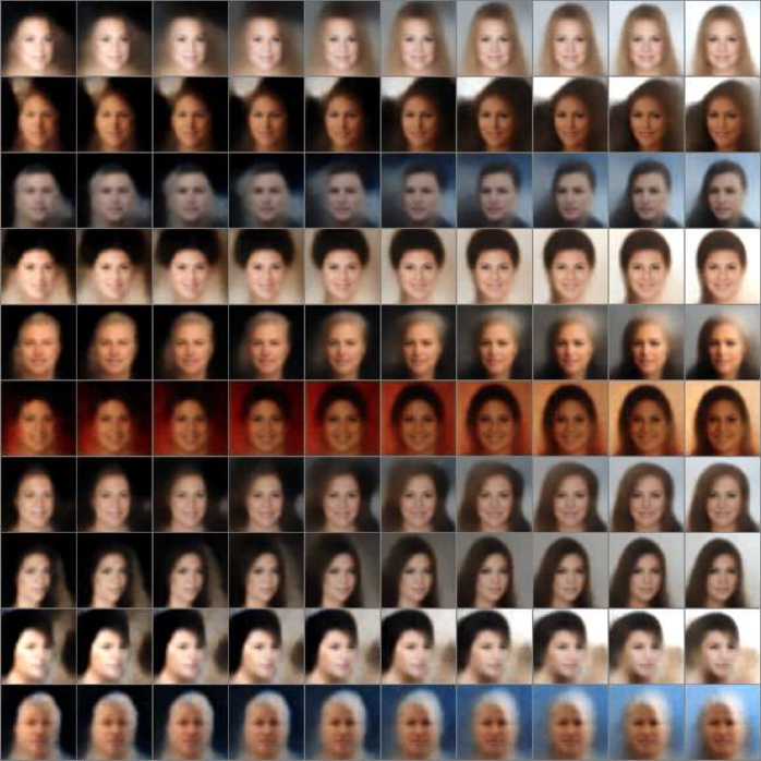
Factor 8: $I(\mathbf{x};{\mathbf{z}_{\mathbf{enc}}}_{8})=0.8$,

$\mathop{\longrightarrow}\limits^{Smile}$

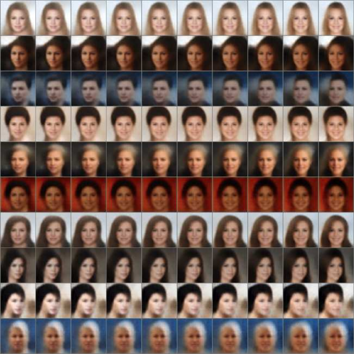
Factor 12: $I(\mathbf{x};{\mathbf{z}_{\mathbf{enc}}}_{12})=2.1$,

$\mathop{\longrightarrow}\limits^{Turn\ Right}$

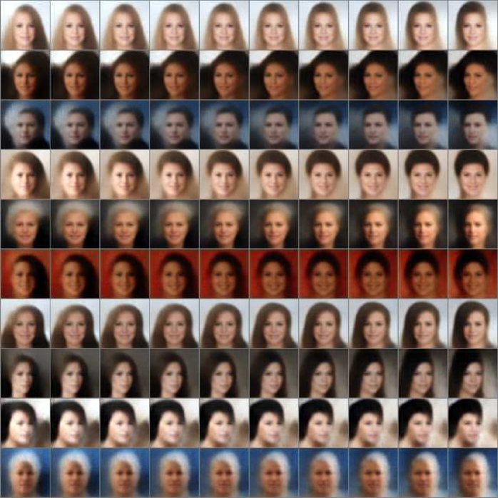
Figure 3: CelebA: Generating Factors Traversal of $\beta$(=40)-VAE. We present the first 3 influential factors determined by estimated mutual information. The whole influential factor traversals are listed in appendix 6.

In order to substantiate the validity of our mutual information estimator, we use it to automatically select influential factors with estimated $I(\mathbf{x};{\mathbf{z}_{\mathbf{enc}}}_{h})>0.5$ of CelebA shown in the Fig.(6) and many of them are possess the interpretable variants such as background color, smile and face angle etc. This verifies that mutual information is an effective indicator to automatically determine the influential factors in VAE setting.

Generation Capability Test for Discovered Factors

Estimated mutual information can instruct the latter generation task with few but influential factors. We select the different ratios of the top influential factors according to the quantity of the mutual information to generate the later image. The factors are sorted according to the values of its mutual information indicators and the other non-influential factors estimated by the indicator are constantly set to zero in the generating process.

Figure 4: Generation plot with different ratio of factors.

According to Fig.(4), we can find that by on using $10\%$ of the top influential factors discovered by the proposed algorithm, the VAE model can still generate images almost similar to the one reconstructed by using whole factors.

Table 1 shows the detailed total information and the reconstruction error corresponding to the different ratio of factor. The top $10\%$ factors contain almost the whole information and therefore their reconstructions have the almost the same reconstruct error compared to using all the factors. As suggested by the information and reconstruction relationship, the less information is contained in the used factors, the higher minimum reconstruction loss bound is raised.

Table 1: mutual information and reconstruction error plot

Top(%) factors in used	100	20	10	7	5	4	3	2	1	0
$I(\mathbf{x};\mathbf{z}_{\mathbf{enc}_{used}})$	24.3	24.3	24.3	19.6	16.5	14.7	10.6	8.4	5.8	0
mean square error	5.6	5.6	5.6	13.4	15.0	18.9	27.6	31.3	44.4	71.7

Classification Capability Test by Discovered Factors

Estimated mutual information can instruct the latter classification task with few but influential factors. We select the different ratio of the top influential factors according to the quantity of the mutual information to predict emotions. The factors are sorted according to its mutual information and the estimated non-influential factors are constantly set to zero in the prediction procedure.

Table 2: Mutual information and EEG-emotion classification with $\beta(=6)$-VAE

Top(%) factors in used	100	50	10	7	5	4	3	2	1	0
$I(\mathbf{x};\mathbf{z}_{\mathbf{enc}_{used}})$	53.8	53.5	38.3	28.0	22.5	19.6	13.5	10.2	7.0	0
mean test accuracy	0.53	0.52	0.46	0.32	0.34	0.36	0.29	0.29	0.3	0.23

According to Table 2, by only using half of the factors, the model still possesses the similar prediction accuracy. Besides, the estimated mutual information on the other side also helps us to determine the several variants which are relevant with the emotion classification as shown in the following Fig.(5).

Factor 1: $I(\mathbf{x};{\mathbf{z}_{\mathbf{enc}}}_{1})=2.1$,

C4-T8-P4-P8  Block,

$\mathop{\longrightarrow}\limits^{\ Red\ Turn\ Green}$

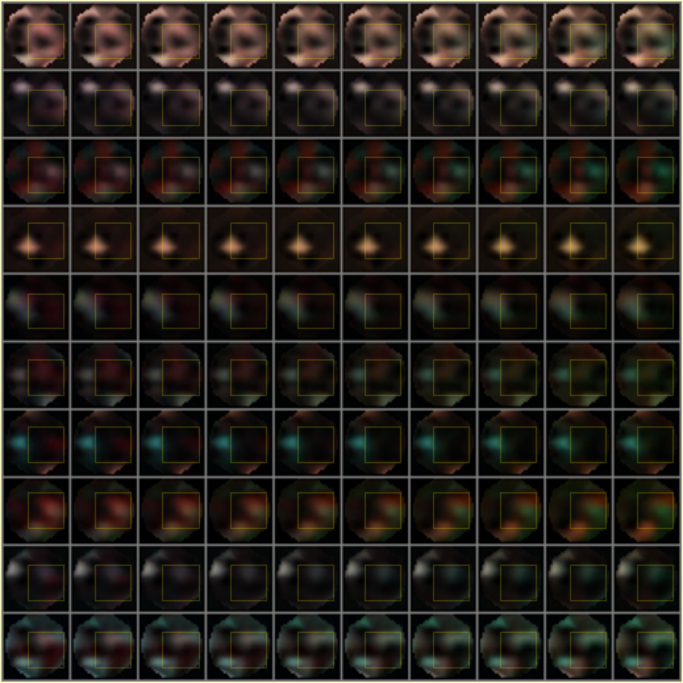
Factor 26: $I(\mathbf{x};{\mathbf{z}_{\mathbf{enc}}}_{104})=3.2$,

PO3-O1-Oz & Fp1-Fp2-AF4-AF3  Block,

$\mathop{\longrightarrow}\limits^{\ Turn\ Dark}$

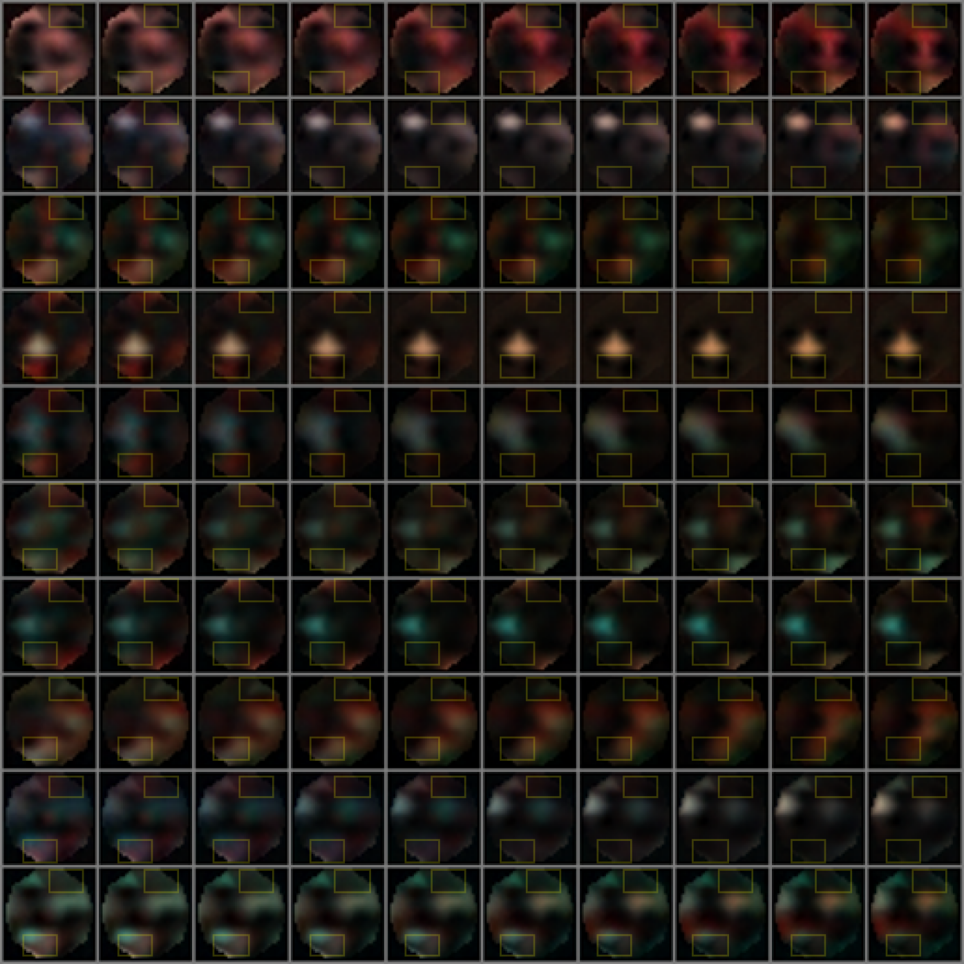
Factor 31: $I(\mathbf{x};{\mathbf{z}_{\mathbf{enc}}}_{113})=3.7$,

PO3-O1-Oz  Block,

$\mathop{\longrightarrow}\limits^{Turn\ Green}$

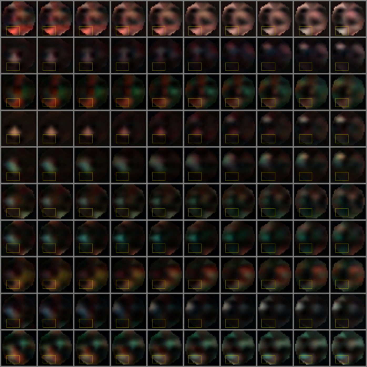
Figure 5: Emotion relevant factors discovery. We present 3 influential factors determined by estimated mutual information. The whole influential factor traversals are listed in Fig.(8) in appendix.

Conclusion

This paper explains the necessity of using mutual information of the input data and each factor as the indicator to estimate the intrinsic influence of a factor to represent data in the VAE model. The mutual information reflects the absolute statistical dependence. The second term in VAE objective and excess pre-set factors inclines to induce the mutual information sparsity and helps achieve influential, as well as ignored, factors in VAE. We have also proved that the mutual information also involves in the lower bound of the mean square error of the reconstruction and of prediction error of the classification. We design a feasible algorithm to calculate the indicator for estimating the mutual information for all factors in VAE and proves its consistency. The experiments show that both the influential factors and non-influential factors can be automatically and effectively found. The interpretability of the discovered factors is substantiated intuitively, and the generalization and classification capability on these factors have also been verified. Specially, some variants relevant to classification are found. The experiments also inspire the idea that we can using a small amount of top influential factors for the latter data processing tasks including generation and classification by still keeping the performance of all factors, just similar to the dimensionality reduction capability as classical PCA, ICA and so on.

The VAE combined with mutual information indicator helps extract knowledge under the data and may be beneficial to extensive latter applications including blind source separation, interpretable feature learning, information bottleneck and data bias elimination. We will investigate these issues in our future research.

Appendix A Appendix A

Theorem 1 (Information Conservation) Suppose that $\mathbf{z}=(z_{1},\cdots,z_{h})$ and $\mathbf{y}=(y_{1},\cdots,y_{P})$ are sets of $H$ and $P$ ($H\neq P$) independent unit Gaussian random variables, respectively, then these two sets of random variables can not be the generating factor of each other. That is, there are no continuous functions $f:\mathbb{R}^{H}\rightarrow\mathbb{R}^{P}$ and $g:\mathbb{R}^{P}\rightarrow\mathbb{R}^{H}$ such that

$$\mathbf{z}=g(\mathbf{y})\quad and\quad\mathbf{y}=f(\mathbf{z}).$$

Proof.

For theorem 1. Proof by Contradiction. Suppose those two function exist, and we will show that they will be inverse mapping of each other and the homeomorphism mapping of $\mathbb{R}^{H}$ and $\mathbb{R}^{P}$. Since $\mathbb{R}^{H}$ and $\mathbb{R}^{P}$ have different topology structures ($P\neq H$), the homeomorphism mapping will not exist.

$\mathbf{z}=g(\mathbf{y})=g(f(\mathbf{z}))$ $\forall\mathbf{z}\in\mathbb{R}^{H}$ $\Rightarrow$ $g\circ f=I_{H}$

$y=f(\mathbf{z})=f(g(\mathbf{x}))$ $\forall\mathbf{y}\in\mathbb{R}^{P}$ $\Rightarrow$ $f\circ g=I_{P}$

Since both $f$ and $g$ are continuous, there is a homeomorphism mapping between $\mathbb{R}^{H}$ and $\mathbb{R}^{P}$ and it leads to the contradiction. ∎

Theorem 2 (Objective Decomposition) If $q_{\mathbf{enc}}(\mathbf{z}|\mathbf{x})\ll p_{\mathbf{dec}}(\mathbf{z})$, i.e., the support of $q_{\mathbf{enc}}(\mathbf{z}|\mathbf{x})$ is contained in support of $p_{\mathbf{dec}}(\mathbf{z})$, for any $\mathbf{x}$, $q_{\mathbf{enc}}(\mathbf{z}|\mathbf{x})=q_{\mathbf{enc}}(z_{1}|\mathbf{x})\cdots q_{\mathbf{enc}}(z_{H}|\mathbf{x})$ and $p_{\mathbf{dec}}(\mathbf{z})=\mathcal{N}(\mathbf{z}|\textbf{0},I_{H})$ then it yields the following decomposition:

• $L_{1}$ norm expression of the KL-divergence term in VAE:

  $$\mathop{{\mathbb{E}}}\limits_{\mathbf{x}\sim p_{data}(\mathbf{x})}D_{KL}(q_{\mathbf{enc}}(\mathbf{z}|\mathbf{x})||p_{\mathbf{dec}}(\mathbf{z}))=\sum_{h=1}^{H}\mathop{{\mathbb{E}}}\limits_{\mathbf{x}\sim p_{data}(\mathbf{x})}D_{KL}(q_{\mathbf{enc}}(z_{h}|\mathbf{x})||p_{\mathbf{dec}}(z_{h}))=$$

  $$\|(\mathop{{\mathbb{E}}}\limits_{\mathbf{x}\sim p_{data}(\mathbf{x})}D_{KL}(q_{\mathbf{enc}}(z_{1}|\mathbf{x})||p_{\mathbf{dec}}(z_{1})),\mathop{{\mathbb{E}}}\limits_{\mathbf{x}\sim p_{data}(\mathbf{x})}D_{KL}(q_{\mathbf{enc}}(z_{2}|\mathbf{x})||p_{\mathbf{dec}}(z_{2})),\cdots,$$

  $$\mathop{{\mathbb{E}}}\limits_{\mathbf{x}\sim p_{data}(\mathbf{x})}D_{KL}(q_{\mathbf{enc}}(z_{h}|\mathbf{x})||p_{\mathbf{dec}}(z_{h})))\|_{1}.$$ (23)

• Further decomposition of an entity in the $L_{1}$ norm expression:

  $$\mathop{{\mathbb{E}}}\limits_{\mathbf{x}\sim p_{data}(\mathbf{x})}D_{KL}(q_{\mathbf{enc}}(z_{h}|\mathbf{x})||p_{\mathbf{dec}}(z_{h}))=I(\mathbf{x};{z_{\mathbf{enc}}}_{h})+D_{KL}(q_{\mathbf{enc}}(z_{h})||p_{\mathbf{dec}}(z_{h})).$$ (24)

Proof.

The $L_{1}$ norm expression is obvious. We prove the further decomposition of an entity in the $L_{1}$ norm expression:

$$\mathop{{\mathbb{E}}}\limits_{\mathbf{x}\sim p_{data}(\mathbf{x})}D_{KL}(q_{\mathbf{enc}}(z_{h}|\mathbf{x})||p_{\mathbf{dec}}(z_{h}))=\int q_{\mathbf{enc}}(z_{h}|\mathbf{x})p_{data}(\mathbf{x})\frac{q_{\mathbf{enc}}(z_{h}|\mathbf{x})p_{data}(\mathbf{x})}{p_{\mathbf{dec}}(z_{h})p_{data}(\mathbf{x})}d\mathbf{x}$$

$$=\int q_{\mathbf{enc}}(z_{h}|\mathbf{x})p_{data}(\mathbf{x})\frac{q_{\mathbf{dec}}(z_{h}|\mathbf{x})p_{data}(\mathbf{x})}{q_{\mathbf{enc}}(z_{h})p_{data}(\mathbf{x})}\frac{q_{\mathbf{enc}}(z_{h})}{p_{\mathbf{dec}}(z_{h})}d\mathbf{x}=I(\mathbf{x};{z_{\mathbf{enc}}}_{h})+D_{KL}(q_{\mathbf{enc}}(z_{h})||p_{\mathbf{dec}}(z_{h})).$$ (25)

∎

Theorem 3 (Mutual Information Separation) Let $z_{1},\cdots,z_{h}$ be independent unit Gaussian distribution, and $z_{1},z_{2},\cdots,z_{h}$ be conditional independent given $\mathbf{x}$. Then

$$I(\mathbf{x};z_{1},\cdots,z_{h})=\sum_{h=1}^{H}I(\mathbf{x};z_{h})=\|(I(\mathbf{x};z_{1}),I(\mathbf{x};z_{2}),\cdots,I(\mathbf{x};z_{h}))\|_{1}.$$ (26)

Proof.

$$I(\mathbf{x};z_{1},\cdots,z_{H})=\int p(z_{1},\cdots,z_{H},\mathbf{x})\log\frac{p(\mathbf{x},z_{1},\cdots,z_{H})}{p(z_{1},\cdots,z_{H})p(\mathbf{x})}dz_{1}\cdots dz_{H}dx$$

$$=\int p(\mathbf{x},z_{1},\cdots,z_{H})\log\frac{\prod_{h=1}^{H}p(z_{h}|\mathbf{x})}{\prod_{h=1}^{H}p(z_{h})}dz_{1}\cdots dz_{H}d\mathbf{x}=\sum_{h=1}^{H}\int p(\mathbf{x},z_{h})\log\frac{p(z_{h}|\mathbf{x})}{p(z_{h})}dz_{h}d\mathbf{x}$$

$$=\sum_{h=1}^{H}I(\mathbf{x};z_{h}).$$

∎

Appendix B Appendix B

MNIST

We split 7000 data points by ratio $[0.6:0.2:0.2]$ into training, validation, testing set. The estimated mutual information and $q^{*}(\mathbf{z})$ are calculated on 10000 data points in the testing set. Seed images from the testing set are used to infer factor value and draw the traversal.

In traversal figures, each block corresponds to the traversal of a single factor over the $[-3,3]$ range while keeping others fixed to their inferred (by $\beta$-VAE, VAE). Each row is generated with a different seed image.

The $\beta$ setting for $\beta$-VAE is enumerated from $[0.1,0.5,1,2:2:18]$.

CelebA

We split randomly roughly 200000 data points by ratio $[0.8:0.1:0.1]$ into training, validation (no use), testing set.

The estimated mutual information and $q^{*}(\mathbf{z})$ are calculated on 10000 data points in the testing set. Seed images from the testing set are used to infer factor value and draw the traversal.

In traversal figures, each block corresponds to the traversal of a single factor over the $[-3,3]$ range while keeping others fixed to their inferred (by $\beta$-VAE, VAE). Each row is generated with a different seed image.

The $\beta$ setting for $\beta$-VAE is enumerated from $[1,30,40]$.

DEAP

DEAP is a well-known public multi-modalities (e.g. EEG, video, etc.) dataset proposed by Koelstra et al. (2012). The EEG signals are recorded from 32 channels by 32 participants watching 40 videos for 63 seconds each. The EEG data was preprocessed which down-sampling into 128Hz and band range 4-45 Hz. By the same transformation idea from Bashivan et al. (2015), we applied fast Fourier transform (FFT) on 1-second EEG signal and convert it to an image. In this experiment, alpha (8-13Hz), beta (13-30Hz) and gamma (30-45Hz) are extracted as the frequency band which represented the activities related to brain emotion emerging. The next step is similar as Bashivan et al. (2015) work which mentioned in section II [PLEASE CHECK IT IN THE PAPER], by Azimuthal Equidistant Projection (AEP) and Clough-Tocher scheme resulting in three 32x32 size topographical activity maps corresponding to each frequency bands shown as RGB plot. The transformation work conduct the total of 1280 EEG videos where each has 63 frames. The two emotional dimensions are arousal and valence, which were labeled from the scale 1-9. For each of them, we applied 5 as the boundary for separating high and low level to generate 4 classes (e.g. high-arousal (HA), high-valence (HV), low-arousal (LA) and low-valence(LV)). In this paper we perform this 4-class classification task as same as the one in [baseline paper].

We split randomly roughly 1280 samples by ratio [0.8: 0.1: 0.1] into training, validation, testing set. $\beta$(= 6)-VAE is trained on each frame and LSTM was used to combine all the frames together for each video.

The estimated mutual information are calculated on 100*63 imagewise(100 videos) data points in the testing set. Seed images from the testing set are used to infer factor value and draw the traversal.

In traversal figures, each block corresponds to the traversal of a single factor over the $[-3,3]$ range while keeping others fixed to their inferred (by $\beta$-VAE). Each row is generated with a different seed image.

Network Structure

Dataset	Optimiser	Architecture
MNIST	Adam	Input	28x28x1
	$1e-3$	Encoder	Conv 32x4x4,32x4x4 (stride 2).
			FC 256. ReLU activation.
	Epoch 200	Latents	128
		Decoder	FC 256. Linear. Deconv reverse of encoder.
			ReLU activation. Gaussian.
CelebA	Adam	Input	64x64x3
	$1e-4$	Encoder	Conv 32x4x4,32x4x4,64x4x4,64x4x4 (stride 2).
			FC 256. ReLU activation.
	Epoch 20	Latents	128/32
		Decoder	FC 256. Linear. Deconv reverse of encoder.
			ReLU activation. Mixture of 2-Gaussian.
DEAP	Adam	Input	32x32x3
	$1e-4$	Encoder	Conv 32x4x4,32x4x4,64x4x4,64x4x4 (stride 2).
			FC 256. ReLU activation.
	Epoch 300	Latents	128/32
		Decoder	FC 256. Linear. Deconv reverse of encoder.
			ReLU activation. Gaussian.
		Input	63x128
		Recurrent	LSTM dim128. Time-Step 63.
		Predictor	FC 4. ReLU activation.

Experiment Plot

In the following subsection, we present the influential factor ($I(\mathbf{x};{\mathbf{z}_{\mathbf{enc}}}_{h})>0.7$) traversals, mutual information and variance plot of different data sets.

i͡n 7,8, 12,13,19,26,28,31,37,40,45,48, 56,63,73,77,81,82,88,90,96,102,110,118,120 Factor -

Figure 6: Mutual Information Sparsity in CelebA: Generating Factors Traversal of $\beta$(=40)-VAE

i͡n 7,22,23,26,30,36,40,47,64,81,91,103,104 Factor -

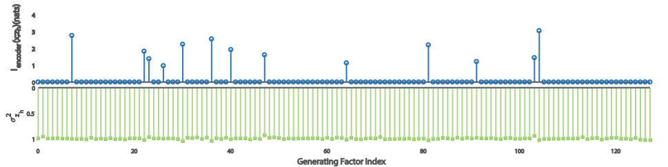
Figure 7: Mutual Information Sparsity in MNIST: Generating Factor Traversal of $\beta$(=10)-VAE

i͡n 1,26,31,36,40,59,60,61,64,65,69,83,86,88,100,104,113,114,116,117 Factor -

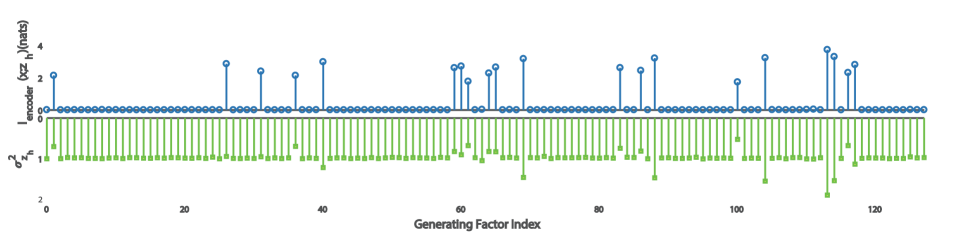
Figure 8: Mutual Information Sparsity in DEAP: Generating Factor Traversal of $\beta$(=6)-VAE

References

- Alemi et al. (2016) Alemi, A. A.; Fischer, I.; Dillon, J. V.; and Murphy, K. 2016. Deep variational information bottleneck. arXiv preprint arXiv:1612.00410.
- Bashivan et al. (2015) Bashivan, P.; Rish, I.; Yeasin, M.; and Codella, N. 2015. Learning representations from eeg with deep recurrent-convolutional neural networks. arXiv preprint arXiv:1511.06448.
- Cover and Thomas (2012) Cover, T. M., and Thomas, J. A. 2012. Elements of information theory. John Wiley & Sons.
- Goodfellow, Bengio, and Courville (2016) Goodfellow, I.; Bengio, Y.; and Courville, A. 2016. Deep learning. MIT press.
- Higgins et al. (2016) Higgins, I.; Matthey, L.; Pal, A.; Burgess, C.; Glorot, X.; Botvinick, M.; Mohamed, S.; and Lerchner, A. 2016. beta-vae: Learning basic visual concepts with a constrained variational framework.
- Higgins et al. (2017a) Higgins, I.; Pal, A.; Rusu, A. A.; Matthey, L.; Burgess, C. P.; Pritzel, A.; Botvinick, M.; Blundell, C.; and Lerchner, A. 2017a. Darla: Improving zero-shot transfer in reinforcement learning. arXiv preprint arXiv:1707.08475.
- Higgins et al. (2017b) Higgins, I.; Sonnerat, N.; Matthey, L.; Pal, A.; Burgess, C. P.; Botvinick, M.; Hassabis, D.; and Lerchner, A. 2017b. Scan: Learning abstract hierarchical compositional visual concepts. arXiv preprint arXiv:1707.03389.
- Hsu, Zhang, and Glass (2017) Hsu, W.-N.; Zhang, Y.; and Glass, J. 2017. Unsupervised learning of disentangled and interpretable representations from sequential data. In Advances in neural information processing systems, 1876–1887.
- Hyvärinen, Karhunen, and Oja (2004) Hyvärinen, A.; Karhunen, J.; and Oja, E. 2004. Independent component analysis, volume 46. John Wiley & Sons.
- Jung et al. (2000) Jung, T.-P.; Makeig, S.; Humphries, C.; Lee, T.-W.; Mckeown, M. J.; Iragui, V.; and Sejnowski, T. J. 2000. Removing electroencephalographic artifacts by blind source separation. Psychophysiology 37(2):163–178.
- Kingma and Welling (2013) Kingma, D. P., and Welling, M. 2013. Auto-encoding variational bayes. arXiv preprint arXiv:1312.6114.
- Koelstra et al. (2012) Koelstra, S.; Muhl, C.; Soleymani, M.; Lee, J.-S.; Yazdani, A.; Ebrahimi, T.; Pun, T.; Nijholt, A.; and Patras, I. 2012. DEAP: A database for emotion analysis; using physiological signals. IEEE Transactions on Affective Computing 3(1):18–31.
- Lécun et al. (1998) Lécun, Y.; Bottou, L.; Bengio, Y.; and Haffner, P. 1998. Gradient-based learning applied to document recognition. Proceedings of the IEEE 86(11):2278–2324.
- Liu et al. (2015) Liu, Z.; Luo, P.; Wang, X.; and Tang, X. 2015. Deep learning face attributes in the wild. In Proceedings of the IEEE International Conference on Computer Vision, 3730–3738.
- Makeig et al. (1996) Makeig, S.; Bell, A. J.; Jung, T.-P.; and Sejnowski, T. J. 1996. Independent component analysis of electroencephalographic data. In Advances in neural information processing systems, 145–151.
- Mathieu et al. (2016) Mathieu, M. F.; Zhao, J. J.; Zhao, J.; Ramesh, A.; Sprechmann, P.; and LeCun, Y. 2016. Disentangling factors of variation in deep representation using adversarial training. In Advances in Neural Information Processing Systems, 5040–5048.
- Peng, Long, and Ding (2005) Peng, H.; Long, F.; and Ding, C. 2005. Feature selection based on mutual information criteria of max-dependency, max-relevance, and min-redundancy. IEEE Transactions on pattern analysis and machine intelligence 27(8):1226–1238.
- Rezende, Mohamed, and Wierstra (2014) Rezende, D. J.; Mohamed, S.; and Wierstra, D. 2014. Stochastic backpropagation and approximate inference in deep generative models. arXiv preprint arXiv:1401.4082.
- Salakhutdinov and Hinton (2009) Salakhutdinov, R., and Hinton, G. 2009. Semantic hashing. International Journal of Approximate Reasoning 50(7):969–978.
- Suzuki, Nakayama, and Matsuo (2016) Suzuki, M.; Nakayama, K.; and Matsuo, Y. 2016. Joint multimodal learning with deep generative models. arXiv preprint arXiv:1611.01891.
- Yang et al. (2004) Yang, J.; Zhang, D.; Frangi, A. F.; and Yang, J.-y. 2004. Two-dimensional pca: a new approach to appearance-based face representation and recognition. IEEE transactions on pattern analysis and machine intelligence 26(1):131–137.