Exoplanets in the Antarctic sky. II. 116 Transiting Exoplanet Candidates Found by AST3-II within the Southern CVZ of TESS

Hui Zhang (张辉) School of Astronomy and Space Science, Key Laboratory of Modern Astronomy and Astrophysics in Ministry of Education,
Nanjing University, Nanjing 210023, Jiangsu,China Zhouyi Yu School of Astronomy and Space Science, Key Laboratory of Modern Astronomy and Astrophysics in Ministry of Education,
Nanjing University, Nanjing 210023, Jiangsu,China Ensi Liang School of Astronomy and Space Science, Key Laboratory of Modern Astronomy and Astrophysics in Ministry of Education,
Nanjing University, Nanjing 210023, Jiangsu,China Ming Yang School of Astronomy and Space Science, Key Laboratory of Modern Astronomy and Astrophysics in Ministry of Education,
Nanjing University, Nanjing 210023, Jiangsu,China Michael C. B. Ashley School of Physics, University of New South Wales, NSW 2052, Australia Xiangqun Cui Nanjing Institute of Astronomical Optics and Technology, Nanjing 210042, China Chinese Center for Antarctic Astronomy, Nanjing 210008, China Fujia Du Nanjing Institute of Astronomical Optics and Technology, Nanjing 210042, China Chinese Center for Antarctic Astronomy, Nanjing 210008, China Jianning Fu Department of Astronomy, Beijing Normal University, Beijing, 100875, China Xuefei Gong Nanjing Institute of Astronomical Optics and Technology, Nanjing 210042, China Chinese Center for Antarctic Astronomy, Nanjing 210008, China Bozhong Gu Nanjing Institute of Astronomical Optics and Technology, Nanjing 210042, China Chinese Center for Antarctic Astronomy, Nanjing 210008, China Yi Hu National Astronomical Observatories, Chinese Academy of Sciences, Beijing 100012, China Chinese Center for Antarctic Astronomy, Nanjing 210008, China Peng Jiang Polar Research Institute of China, Shanghai 200136, China Chinese Center for Antarctic Astronomy, 451 Jinqiao Rd, Nanjing 210008, China Huigen Liu School of Astronomy and Space Science, Key Laboratory of Modern Astronomy and Astrophysics in Ministry of Education,
Nanjing University, Nanjing 210023, Jiangsu,China Jon Lawrence Australian Astronomical Optics, Macquarie University, NSW 2109, Australia Qiang Liu National Astronomical Observatories, Chinese Academy of Sciences, Beijing 100012, China Xiaoyan Li Nanjing Institute of Astronomical Optics and Technology, Nanjing 210042, China Chinese Center for Antarctic Astronomy, Nanjing 210008, China Zhengyang Li Nanjing Institute of Astronomical Optics and Technology, Nanjing 210042, China Chinese Center for Antarctic Astronomy, Nanjing 210008, China Bin Ma National Astronomical Observatories, Chinese Academy of Sciences, Beijing 100012, China Chinese Center for Antarctic Astronomy, Nanjing 210008, China University of Chinese Academy of Sciences, Beijing 100049, China Jeremy Mould Centre for Astrophysics and Supercomputing, Swinburne University of Technology, PO Box 218, Mail Number H29, Hawthorn, VIC 3122, Australia ARC Centre of Excellence for All-sky Astrophysics (CAASTRO) Zhaohui Shang Tianjin Astrophysics Center, Tianjin Normal University, Tianjin 300387, China National Astronomical Observatories, Chinese Academy of Sciences, Beijing 100012, China Chinese Center for Antarctic Astronomy, Nanjing 210008, China Nicholas B. Suntzeff George P. and Cynthia Woods Mitchell Institute for Fundamental Physics & Astronomy, Texas A. & M. University,
Department of Physics and Astronomy, 4242 TAMU, College Station, TX 77843, US Charling Tao Aix Marseille Univ, CNRS/IN2P3, CPPM, Marseille, France Physics Department and Tsinghua Center for Astrophysics (THCA), Tsinghua University, Beijing, 100084, China Qiguo Tian Polar Research Institute of China, 451 Jinqiao Rd, Shanghai 200136, China C. G. Tinney Exoplanetary Science at UNSW, School of Physics, UNSW Sydney, NSW 2052, Australia Syed A. Uddin Purple Mountain Observatory, Nanjing 210008, China Lifan Wang George P. and Cynthia Woods Mitchell Institute for Fundamental Physics & Astronomy, Texas A. & M. University,
Department of Physics and Astronomy, 4242 TAMU, College Station, TX 77843, US Purple Mountain Observatory, Nanjing 210008, China Chinese Center for Antarctic Astronomy, Nanjing 210008, China Songhu Wang Department of Astronomy, Yale University, New Haven, CT 06511, USA Xiaofeng Wang Physics Department and Tsinghua Center for Astrophysics (THCA), Tsinghua University, Beijing, 100084, China Peng Wei School of Astronomy and Space Science, Key Laboratory of Modern Astronomy and Astrophysics in Ministry of Education,
Nanjing University, Nanjing 210023, Jiangsu,China Duncan Wright University of Southern Queensland, Computational Engineering and Science Research Centre, Toowoomba, Queensland 4350, Australia Xuefeng Wu Purple Mountain Observatory, Nanjing 210008, China Chinese Center for Antarctic Astronomy, Nanjing 210008, China Robert A. Wittenmyer University of Southern Queensland, Computational Engineering and Science Research Centre, Toowoomba, Queensland 4350, Australia Lingzhe Xu Nanjing Institute of Astronomical Optics and Technology, Nanjing 210042, China Shi-hai Yang Nanjing Institute of Astronomical Optics and Technology, Nanjing 210042, China Chinese Center for Antarctic Astronomy, Nanjing 210008, China Ce Yu School of Computer Science and Technology, Tianjin University, Tianjin 300072, China Xiangyan Yuan Nanjing Institute of Astronomical Optics and Technology, Nanjing 210042, China Chinese Center for Antarctic Astronomy, Nanjing 210008, China Jessica Zheng Australian Astronomical Observatory, 105 Delhi Road, North Ryde, NSW 2113, Australia Hongyan Zhou Polar Research Institute of China, 451 Jinqiao Rd, Shanghai 200136, China Ji-lin Zhou School of Astronomy and Space Science, Key Laboratory of Modern Astronomy and Astrophysics in Ministry of Education,
Nanjing University, Nanjing 210023, Jiangsu,China Zhenxi Zhu Purple Mountain Observatory, Nanjing 210008, China Chinese Center for Antarctic Astronomy, Nanjing 210008, China

Abstract

We report first results from the CHinese Exoplanet Searching Program from Antarctica (CHESPA)—a wide-field high-resolution photometric survey for transiting exoplanets carried out using telescopes of the AST3 (Antarctic Survey Telescopes times 3) project. There are now three telescopes (AST3-I, AST3-II, and CSTAR-II) operating at Dome A—the highest point on the Antarctic Plateau—in a fully automatic and remote mode to exploit the superb observing conditions of the site, and its long and uninterrupted polar nights. The search for transiting exoplanets is one of the key projects for AST3. During the austral winters of 2016 and 2017 we used the AST3-II telescope to survey a set of target fields near the southern ecliptic pole, falling within the continuous viewing zone of the TESS mission (Ricker et al., 2010). The first data release of the 2016 data, including images, catalogs and lightcurves of 26578 bright stars ( $7.5\leq\textbf{{m}}_{\textit{i}}\leq 15$ ) was presented in Zhang et al. (2018). The best precision, as measured by the RMS of the lightcurves at the optimum magnitude of the survey ( $\textbf{{m}}_{\textit{i}}=10$ ), is around 2 mmag. We detect 222 objects with plausible transit signals from these data, 116 of which are plausible transiting exoplanet candidates according to their stellar properties as given by the TESS Input Catalog (Stassun et al., 2017), Gaia DR2 (Gaia Collaboration et al., 2018) and TESS-HERMES spectroscopy (Sharma et al., 2018). With the first data release from TESS expected in late 2018, this candidate list will be a timely for improving the rejection of potential false positives.

planets and satellites: detection — binaries: eclipsing — stars: variables: general — surveys — techniques: photometric — catalogs

^†^†journal: ApJS^†^†software: Swarp (Bertin et al., 2002), VARTOOLS (Hartman & Bakos, 2016), MATLAB

1 Introduction

The rapidly expanding sample size of exoplanets discovered over the last two decades has allowed entirely new classes of study of planetary demographics, and has dramatically expanded our understanding of the distribution of planetary orbital parameters. To further increase this understanding, more exoplanet detections covering a wider parameter space are required—and in particular more detections of planets orbiting host stars bright enough for ground-based follow-up to measure dynamical masses. The TESS mission’s satellite (Ricker et al., 2010) was launched successfully in April 2018, and is expected to produce a substantial crop of exactly this class of exoplanets (Stassun et al., 2017), allowing it to have potentially even larger impact than the Kepler (Borucki et al., 2010) and CoRoT (Auvergne et al., 2009) missions.

In advance of these substantial detections of exoplanets by space telescopes, the first transiting exoplanets were discovered by ground-based, small-aperture telescopes, and these facilities have continued to operate in parallel over the last decade, delivering hundreds of exoplanets from projects including HATNET (Bakos et al., 2004), WASP/SuperWASP (Pollacco et al., 2006), HATSouth (Bakos et al., 2013), and KELT (Pepper et al., 2007). The common features of these ground-based searching programs have been the use of Small-apertures, Wide-fields, and Arrays of Telescopes (Hereafter the SWAT). And the SWAT have been proved to be one of the most efficient and economical ways to search for new transiting exoplanets from the ground.

However, photometric surveys using ground-based SWATs suffer from two major drawbacks compared to space-based surveys: lower photometric precision and lower duty-cycle coverage. As present and future space-based wide-field surveys continue to progress, from Kepler and CoRoT to TESS to PLATO2.0 (Barban13; Rauer et al., 2014), these drawbacks have called the value of the ground-based SWAT facilities into question. Ground-based SWAT surveys have to improve their capabilities and work in partnership with present and future space-based wide-field surveys to achieve the greatest impact. On one hand, as experience has been gained and new technologies adopted, new generation wide-field transit searching programs such as NGTS (Wheatley et al., 2018) and Pan-Planets (Obermeier et al., 2016) have been pushing photometric precision to levels precision (i.e., a few millimagnitudes). Their experience has shown that instruments that are stable over the long-term, combined with optimized operations (e.g., precision auto-guiding) are critical for improving long-term photometric precision. On the other hand, choosing a good site with superb observing conditions (e.g., a steady atmosphere and a clear dark sky) is also essential to guaranteeing an efficient observing by a ground-based SWAT facility.

Because of its extremely cold, dry, and clear atmosphere, the Antarctic Plateau provides favorable conditions for optical, infrared and THz astronomical observations. (Lawrence et al., 2004) reported a median seeing of $0.23^{\prime\prime}$ (average of $0.27^{\prime\prime}$ ) above a 30 m boundary layer at Dome C, drawing world-wide attention. Subsequently, many studies have been focused on the astronomical conditions at a variety of Antarctic sites, and have shown low sky brightness and extinction (Kenyon & Storey, 2006; Zou et al., 2010; Yang et al., 2017), low water vapor (Shi et al., 2016), very low wind speeds, and exceptional seeing above a thin boundary layer (Bonner et al., 2010; Okita et al., 2013; Hu et al., 2014; Aristidi et al., 2009; Fossat et al., 2010; Giordano et al., 2012). Furthermore, the decreased high-altitude turbulence above the plateau results in reduced scintillation noise, further improving photometric precision (Kenyon & Storey, 2006). Saunders et al. (2009) studied eight major factors, such as the boundary layer thickness, cloud coverage, auroral emission, airglow, atmospheric thermal backgrounds, precipitable water vapor, telescope thermal backgrounds, and the free-atmosphere seeing, at Domes A, B, C and F, and also Ridge A and B. After a systematic comparison, they concluded that Dome A, the highest point of the Antarctic Plateau, would be the best site overall.

In addition to the excellent photometric conditions at Dome A, the small variation in the elevation of targets as they track around the sky at Dome A will reduce the systematics. And most importantly, the uninterrupted polar nights offer an opportunity to obtain nearly continuous photometric monitoring for periods of more than a month. As shown by a series of previous studies (Crouzet et al., 2010; Daban et al., 2010; Law et al., 2013), this greatly increases the detectability of transiting exoplanets with orbital periods longer than a few days. The outstanding photometric advantages of the Antarctic Plateau have been shown by the observing facilities at different sites, such as SPOT (Taylor et al., 1988) at the South Pole, the small-IRAIT (Tosti et al., 2006), ASTEP-South (Crouzet et al., 2010) and ASTEP-400 (Daban et al., 2010; Mékarnia et al., 2016) at Dome C, and CSTAR (Wang et al., 2011, 2014; Yang et al., 2015; Zong et al., 2015; Oelkers et al., 2016; Liang et al., 2016) and AST3-I (Wang et al., 2017; Ma et al., 2018) at Dome A.

To utilize the superb observing conditions, the construction of a remote observatory at Dome A commenced in 2008, with the installation of a first generation telescope CSTAR (the Chinese Small Telescope ARray, Yuan et al., 2008; Zhou et al., 2010). Based on a successful experience with CSTAR (and the lessons learned from it), a second generation of survey telescopes—the AST3 telescopes (Antarctic Survey Telescopes times 3, Cui et al., 2008; Yuan et al., 2014)—were conceived to implement wide-field high-resolution photometric surveys at Dome A. The first and second AST3 telescopes—AST3-I and AST3-II—were installed at Dome A in 2012 and 2015 by the 28th and 29th CHINARE (CHInese National Antarctic Research Expeditions), respectively. Using the CSTAR and AST3 telescopes, we have been running an exoplanet survey program called CHESPA (the CHinese Exoplanet Searching Program from Antarctica). The primary science goal of CHESPA is finding Super-Earth or Neptune-sized transiting exoplanets around a variety of host-star stellar types that are sufficiently bright for radial velocity confirmation and dynamical mass measurement. The combination of dynamical masses and planetary sizes will allow us to determine the true masses, orbital eccentricities, and most critically their bulk densities. With accurate physical and dynamic properties determined, these exoplanets will be good targets for a wide range of characterization techniques, e.g., studies of their atmospheric structure and composition (see, e.g., Seager et al., 2007; Baraffe et al., 2008). The first six exoplanet candidates around the South Celestial Pole were reported by Wang et al. (2014), and (although not yet confirmed) they demonstrate the potential power of CHESPA for the discovery of new exoplanets.

Although the basic design of CHESPA is much the same as most other ground-based SWAT facilities, we do have a few additional advantages over other, similar surveys: a large FoV combined with a relatively high angular resolution of $1^{\prime\prime}$ pixel^-1, multi-band filters, and superb observing conditions from Antarctica. To maximize our linkage with upcoming space-based surveys like TESS, we have scheduled our ongoing survey to make observations that scan TESS’ high-value target zones, but with a higher angular resolution and in a different filter (Sloan $i$ -band). During the austral winters of 2016 and 2017, we have surveyed two sets of fields selected within the Southern Continuous Viewing Zone (CVZ) of TESS (Ricker et al., 2010) using AST3-II. The remaining target fields will be scanned in 2019. The reason we choose these fields is that the stars in the CVZ will be over a 13 times longer observing period than most of objects of the TESS survey (i.e. continuously over a full year). Hence, light curves for objects in the CVZ will be much more sensitive to small planets in short-period orbits (Stassun et al., 2017), as well as sensitive to larger planets with orbits with much longer periods. In addition, the TESS CVZ and the JWST CVZ are both over the same area of sky (i.e. the south ecliptic pole), so planets detected in these overlapping regions will have enormous potential for further detailed follow-up to characterize in detail their atmosphere and internal structure.

Zhang et al. (2018) has presented the first release of 2016 data from AST3-II, as well as a catalog of 221 newly discovered variables. In this paper, we present the detection of 116 transiting exoplanet candidates from the same data. As more data are returned from Antarctica, new results will be presented in forthcoming papers. In this work, we introduce the AST3-II facility in Section 2 and describe the observations of CHESPA briefly in Section 3; in Section 4 we detail the data reduction pipeline, including lightcurve detrending, transit signal searching, and the transit signal validation software modules; finally, we present the survey results in Section 5 and summarize the paper in Section 6.

2 Instruments

Detailed descriptions of the AST3 telescopes have been previously presented by Cui et al. (2008); Yuan et al. (2014, 2015); Wang et al. (2017). Here we only focus on the key properties of the AST3-II telescope. The AST3-II telescope (which acquired all the data presented in this paper) has an effective aperture of 50 cm. It is designed to obtain wide-field ( $1.5\times 2.9\mbox{ deg}^{2}$ in RA $\times$ Dec) and high resolution ( $\approx 1^{\prime\prime}$ pixel^-1) imaging in the Sloan $i$ -band. It employs a modified Schmidt optical design (Yuan & Su, 2012) and a $10\mbox{K}\times 10\mbox{K}$ pixel frame transfer STA1600FT CCD camera. To withstand the extremely harsh environment at Dome A, careful design work has been done to implement multiple innovations in the telescope’s snow-proofing and defrosting systems. As a result, AST3-II worked well during the extremely cold austral winters of 2016 and 2017, and acquired over 30 TB of high-quality images. During the observational seasons in austral winter, AST3-II is operated remotely and the scheduled observations are executed in a fully-automatic mode. The hardware and software for the facility—including the hardware operation monitor, telescope control computer, and data storage array—were developed by the National Astronomical Observatories, Chinese Academy of Sciences (NAOC) (Shang et al., 2012; Hu et al., 2016). The electrical power supply and internet communication were provided by a similarly reliable on-site observatory platform, PLATO-A, which is an improved version of the PLATO system developed by UNSW Sydney as an automated observatory platform for CSTAR and other earlier instruments. PLATO-A was designed to provide a continuous 1 kW power source, a warm environment for equipment, and internet communications to the AST3 telescopes for a year without servicing (Lawrence et al., 2009; Ashley et al., 2010).

3 Observations

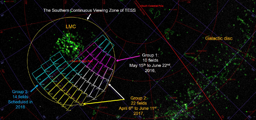
The scientific background and observational strategy of CHESPA are described in Zhang et al. (2018). We summarize the key points here. The CHESPA program is dedicated to searching for transiting exoplanets in the southern polar sky at highly negative declinations. It has been running since 2012 using the CSTAR and AST3 telescopes, with a first batch of six exoplanet candidates published by Wang et al. (2014). To maximize collaboration with TESS and enhance the scientific importance of our searching program, we selected 48 target fields close to the South Ecliptic Pole ( $\mbox{RA}=06^{\mbox{h}}\,00^{\mbox{m}}\,00^{\mbox{s}},\mbox{Dec}=-66^{\circ}\,33^{\prime}\,00^{\prime\prime}$ ) and within the TESS’ Southern CVZ (Continuous Viewing Zone) (see Figure 1 and Table 1 for details). All target fields are and are suitable for low-airmass observation from Antarctica. Target stars located in these fields will also be monitored by TESS for continuous 12 month period. Thus, any candidate of interest found within these fields may be followed up and studied thoroughly in the future.

Table 1: Center coordinates of the 48 AST3-II target fields surveyed/scheduled in 2016–2019.

Field Name	Field Center		Observation Date	Valid Images
	RA(J2000)	Dec(J2000)
AST3II001	$93.000$	$-76.000$	2018–2019
AST3II002	$99.000$	$-76.000$	2018–2019
AST3II003	$105.000$	$-76.000$	2018–2019
AST3II004	$93.000$	$-73.000$	2016.05.15–2016.06.22	3179
AST3II005	$98.500$	$-73.000$	2016.05.15–2016.06.22	3080
AST3II006	$104.000$	$-73.000$	2016.05.15–2016.06.22	3049
AST3II007	$109.500$	$-73.000$	2016.05.15–2016.06.22	3103
AST3II008	$115.000$	$-73.000$	2016.05.15–2016.06.22	3248
AST3II009	$93.000$	$-70.000$	2016.05.15–2016.06.22	3090
AST3II010	$97.750$	$-70.000$	2016.05.15–2016.06.22	3000
AST3II011	$102.500$	$-70.000$	2016.05.15–2016.06.22	2991
AST3II012	$107.250$	$-70.000$	2016.05.15–2016.06.22	3021
AST3II013	$112.000$	$-70.000$	2016.05.15–2016.06.22	3128
AST3II014	$116.750$	$-70.000$	2017.04.06–2017.05.12	$\geq 3000$
AST3II015	$93.000$	$-67.000$	2018–2019
AST3II016	$97.000$	$-67.000$	2018–2019
AST3II017	$101.000$	$-67.000$	2017.04.06–2017.05.12	$\geq 3000$
AST3II018	$105.000$	$-67.000$	2017.04.06–2017.05.12	$\geq 3000$
AST3II019	$109.000$	$-67.000$	2017.04.06–2017.05.12	$\geq 3000$
AST3II020	$113.000$	$-67.000$	2017.04.06–2017.05.12	$\geq 3000$
AST3II021	$117.000$	$-67.000$	2017.04.06–2017.05.12	$\geq 3000$
AST3II022	$82.500$	$-64.000$	2018–2019
AST3II023	$86.000$	$-64.000$	2018–2019
AST3II024	$89.500$	$-64.000$	2018–2019
AST3II025	$93.000$	$-64.000$	2018–2019
AST3II026	$96.500$	$-64.000$	2018–2019
AST3II027	$100.000$	$-64.000$	2017.04.06–2017.05.12	$\geq 3000$
AST3II028	$103.500$	$-64.000$	2017.04.06–2017.05.12	$\geq 3000$
AST3II029	$107.000$	$-64.000$	2017.04.06–2017.05.12	$\geq 3000$
AST3II030	$110.500$	$-64.000$	2017.04.06–2017.05.12	$\geq 3000$
AST3II031	$114.000$	$-64.000$	2017.04.06–2017.05.12	$\geq 3000$
AST3II032	$83.250$	$-61.000$	2018–2019
AST3II033	$86.500$	$-61.000$	2018–2019
AST3II034	$89.750$	$-61.000$	2018–2019
AST3II035	$93.000$	$-61.000$	2017.05.14–2017.06.11	$\geq 4100$
AST3II036	$96.250$	$-61.000$	2017.05.14–2017.06.11	$\geq 4100$
AST3II037	$99.500$	$-61.000$	2017.05.14–2017.06.11	$\geq 4100$
AST3II038	$102.750$	$-61.000$	2017.05.14–2017.06.11	$\geq 4100$
AST3II039	$106.000$	$-61.000$	2017.05.14–2017.06.11	$\geq 4100$
AST3II040	$109.250$	$-61.000$	2017.05.14–2017.06.11	$\geq 4100$
AST3II041	$84.000$	$-58.000$	2018–2019
AST3II042	$87.000$	$-58.000$	2018–2019
AST3II043	$90.000$	$-58.000$	2018–2019
AST3II044	$93.000$	$-58.000$	2017.05.14–2017.06.11	$\geq 4100$
AST3II045	$96.000$	$-58.000$	2017.05.14–2017.06.11	$\geq 4100$
AST3II046	$99.000$	$-58.000$	2017.05.14–2017.06.11	$\geq 4100$
AST3II047	$102.000$	$-58.000$	2017.05.14–2017.06.11	$\geq 4100$
AST3II048	$105.000$	$-58.000$	2017.05.14–2017.06.11	$\geq 4100$

These chosen fields are divided into three groups, each of which was originally scheduled for observation over an austral winter in 2016, 2017, and 2018. From 2016 May 16 to 2016 June 22 in 2016, we observed the first group consisting of 10 fields (AST3II004–AST3II013). The second group comprises 22 fields and observed from 2017 April 6 to 2017 June 11 (see Table 1 for details). The ten 2016 fields were monitored by the AST3-II telescope for over 350 hours, spanning 37 available or half-available nights. (The remaining time was allocated to instrument maintenance and used for other key projects, including a supernova search.) To avoid saturating bright stars, and to maximize the survey’s dynamic range, we adopted a short-exposure-stacking strategy. The 10 target fields were scanned one by one in a loop with three consecutive 10 s exposures being taken in each field, before moving on to the next field. The resulting sampling cadence is about 12 minutes for each field, including the dead time caused by slewing ( $\sim 24$ s) and CCD readout ( $\sim 48$ s). Twilight sky frames were taken at each dawn and dusk during the periods when the Sun was still rising and setting from Dome A. These frames were then median-combined to produce a master flat-field image. To reduce the systematic errors caused by the imperfection of the flat-field correction, we adjusted the focus of the optics to sample stars with point-spread function sizes between $\mbox{FWHM}=3$ pixels to $\mbox{FWHM}=5$ pixels, while the pixel-scale of AST3-II is $1^{\prime\prime}$ pixel^-1, which is designed to match the average seeing at Dome A within the boundary layer. We made template images for each target field, and determined accurate astrometric solutions. Every time the telescope points to a new field, any small offsets in RA and Dec are corrected by cross-matching the first image with the template, and correcting pointing for the second and third images. Then the last two frames are resampled and matched to the first one to guarantee pixel alignments. At last, all three pixel-aligned images are median combined by the Swarp code (Bertin et al., 2002) to produce a new image.

During 2016, over 35000 science images in our 10 target fields were acquired by AST3-II and brought back on hard disks by the 33rd CHINARE team. The first data release, including 18729 coadded images/catalogs and 26578 lightcurves of stars brighter than 15th magnitude in the Sloan $i$ -band were presented in Zhang et al. (2018). In 2017, more than 80000 images were taken and we await the return of this data from the next polar servicing expedition. In 2018, however, due to some technical problems, no expedition was sent to the Kunlun station. And the scheduled CHESPA 2018 survey was canceled after the on-site fuel storage was exhausted.

Refer to caption — Figure 1: Scheduled survey of 48 target fields in 2016, 2017, and 2018. Each field has a sky coverage of $\sim 4.3$ deg². Fields close to the LMC are excluded to avoid crowded fields of giant stars. Group 1 (10 fields) and group 2 (22 fields) have been scanned in 2016 and 2017, respectively.

3.1 Detection Probability versus Orbital Period

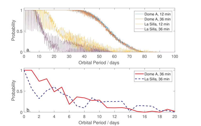
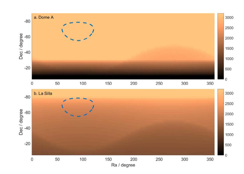
To demonstrate the advantages of Antarctica for finding transiting exoplanets within the Southern CVZ of TESS, we simulated the relation between the orbital period of a transiting exoplanet and its probability of being found at two sites: Dome A and La Silla (i.e. a representative temperate-latitude observing site with good weather and seeing). The simulated observation campaign lasts from the beginning of April to the end of September, which covers the entire austral winter from Dome A. We assume the fraction of bad weather to be $20\%$ at both sites. Two sampling cadences are adopted—12 and 36 minutes—consistent with our Dome A observing strategies. In addition, we performed simulations implementing the actual real-time epochs of observation from our 2016 data. Due to some technical failures caused by the harsh environment at Dome A, the observation in 2016 ended in the end of June and the overall operation coverage is around $\sim 40\%$ which is much less than the coverage we expected: $\sim 75\%$ . As a result, the detection probability in 2016 is not quite improved and it is even worse at the long-period end. The results are shown in Figure 2. The detection probability of a transiting planet is calculated following the method of Beatty & Gaudi (2008). These figures highlight three key features. First, that the limited amount of actual data obtained in 2016 does not have significantly different sensitivity from a temperature latitude site. But, that more extended continuous observations with no diurnal gaps (i.e. from Dome A) massively improves the efficiency of the detection of planets at periods of longer than $\sim$ 10 d. And finally, that when observing at Dome A the choice of a 12 minute or 36 minute cadence makes little difference to the detectability of planets out to orbital periods of $\sim$ 40 d. Figure 3 shows the total available hours as a function of position on the sky as visible from Dome A and La Silla. The dashed circle shows the position of the Southern CVZ of TESS, which can clearly be monitored for a much longer period from Dome A, making the detection of planets at periods of 30-40 d feasible from Dome A.

4 Transit Signal Searching Pipeline

A detailed description of the “Image Reduction Module” is provided in Zhang et al. (2018), including the standard image processing steps (e.g., the 2-D over-scan subtraction, flat-field correction, zero-point magnitude correction), plus some treatments unique to our data (e.g., cross-talk correction and electromagnetic interference noise fringe correction). In this paper we focus on the lightcurve production process which comprises “Lightcurve Detrending”, “Transit Signal Searching”, and “Transit Signal Validation” modules.

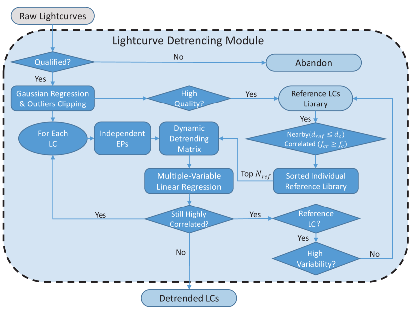
4.1 Lightcurve Detrending Module

Wide-field photometry surveys usually suffer from serious systematic errors, e.g., scattered light, imperfect flat-fields, and tracking errors. To identify all sources of such systematics and remove them is not an easy task and sometimes is not even feasible (Mékarnia et al., 2016). The widely-used simple ensemble photometry (e.g., Honeycutt, 1992) assumes that all stars in the field are affected by the same systematics (e.g., transparency changes), and can be modeled by averaging out all incoming fluxes from the ensemble (or selected reference stars). However, even when color and spatial terms due to differential extinction are applied, systematic errors remain. To reveal tiny transit signals (e.g., $\lesssim 1\%$ ) it is essential to reach photometric precisions of a few mmag (RMS). This task is approaching the fundamental limits for ground-based photometry surveys and requires further treatments of systematics.

Modern algorithms for systematic filtering assume that while systematic errors are specific to each star, they can be modeled by a linear combination of the systematics of selected reference stars and auxiliary measurable quantities such as the centroid position and width of the point spread function (Bakos et al., 2007). The determination of coefficients for this linear combination is usually performed by standard least-squares techniques. Two kinds of method have been extensively used in the data reduction of wide-field photometric surveys: SYSREM (SYStematic effects REMove, Tamuz et al., 2005) and TFA (Trend Filtering Algorithm, Kovács et al., 2005). These approaches have been proved to be effective against systematic errors from unknown sources and are also known as “blind-detrending” algorithms. However, sometimes they are too effective: to reach a high precision (i.e., low RMS) lightcurves are often “flattened out” to the extent that there may be substantial suppression of the signals we are searching for. The success of this kind of methods is quite dependent on the selection of the reference stars. TFA (for example) uses a “brute force” fit of many selected template stars from the target field; if the number of template stars is too small, the detrending procedure may be ineffective, while if the number of template stars is too large, the procedure is very time-consuming and the target lightcurve may be “over-fitted” with all real physical variations removed (Kovács et al., 2016).

On one hand, we need to remove all unwanted signals (systematics). On the other hand, we have to retain the strength of all wanted (transit) signals. Many efforts have been made to achieve a balance between these conflicting requirements. One approach is to run the filtering methods in the “signal-reconstructive” mode, once the signal frequency (in the case of TFA) or basis of trends (in the case of SysRem) is determined (Kovács & Bakos, 2007). Another approach is based on a careful selection of the template time series. Kim et al. (2009) used a hierarchical clustering method to select an optimum number of co-trending lightcurves. A PCA-based criterion is used in the algorithm proposed by Petigura & Marcy (2012) for the analysis of the Kepler lightcurves. The more involved PDC-MAP pipeline (Stumpe et al., 2012; Smith et al., 2012) of the Kepler mission also utilizes PCA for selecting the basis vectors for the correction of systematics. In a similar manner, Roberts et al. (2013) discuss the advantage of using Bayesian linear regression for robust filtering, and employing an entropy criterion for selecting the most relevant corrections.

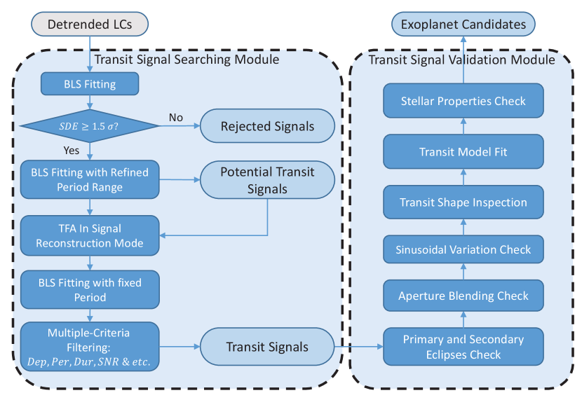
We implement a TFA-based algorithm with both a signal-reconstructive mode and an optimal-template selection. The detailed process is composed of the following steps (flow chart is shown in Figure 4):

Step I. filter out non-physical outliers: these outliers, caused mainly by mis-matches of stars or bad weather, will cause serious problems in the following detrending processes. Occasionally they may also crash the BLS (Box-function Least Square Fitting algorithm Kovács et al., 2002) procedure when searching for transit signals. To eliminate these outliers while retaining the time-dependent astrophysical variations, the mean magnitude is subtracted from each lightcurve and a Gaussian Process Regression (GPR) model is fitted to the mean-subtracted measurements. GPR is a nonparametric kernel-based probabilistic method that can be used to predict responses of a function with multiple variables when a kernel function is given. A description of GPR models and their application in removing multi-variate systematics and intrinsic variations from lightcurve can be found in (Aigrain et al., 2016). In our case, we simply set the observation time, $t_{i}$ , as the only variate, and consider the following model of the magnitude response $m_{i}$ :

m_{i}=t_{i}\beta+\textit{f}_{i}(t),i=1,2,3...N_{obs},

(1)

where $N_{obs}$ is the number of observations and $\textit{f}_{i}(t)\sim\text{GP}(0,\textbf{K})$ , that is $\textit{f}_{i}(t)$ are from a zero mean Gaussian Process with covariance matrix $\textbf{K}_{ij}=k_{t}(t_{i},t_{j})$ . To model the time-dependent variation, a squared exponential kernel function is adopted:

k_{t}(t_{i},t_{j})=A_{t}exp[-\alpha(t_{i}-t_{j})^{2}].

(2)

The amplitude $A_{t}$ and coefficients $\beta$ and $\alpha$ are estimated directly from the time series by a build-in function ”fitrgp” of $\emph{\text{MATLAB}}^{T}$ . All measurements that are $3\sigma$ away from this GPR fitted model are clipped. Note that the fitted model is not subtracted from the observations at this step.

Step II. Build a target list and a reference star library: the target list contains all lightcurves with magnitude $\textbf{{m}}_{\textit{i},apass}\leq 15.0$ ; the reference library contains all the stars with lightcurves having a completeness of observations greater than $90\%$ and magnitudes ranging from $\textbf{{m}}_{\textit{i},apass}=10$ to $\textbf{{m}}_{\textit{i},apass}=14$ .

Step III. Build a template for each lightcurve about to be detrended: reference stars in the individual template are selected from the reference library according to several criteria: i. the RMS of a reference lightcurve should be less than the median value of all lightcurves; ii. the angular distance between a reference star and the target should be less than $1.0^{\circ}$ to ensure they have been affected by similar kinds of systematics; iii. reference stars that are too close to the target ( $\leq 30.0^{\prime\prime}$ ) are removed to avoid self-detrending; iv. the brightness variation of a reference star should be highly correlated with that of the target. In practice we calculate the Pearson correlation coefficient (PCC) between the target lightcurve and each valid reference lightcurve, with the top $N_{\text{ref}}$ reference lightcurves with $\text{PCC}>0.2$ being selected; v. A reference star located within the same readout channel with the target star has a higher priority to be selected. If the number of valid stars within the same readout channel is less than the required number, $N_{\text{ref}}$ , we supplement the reference stars with those in nearby readout channels.

Step IV. Build individual trend matrices for each target lightcurve: each trend matrix contains two kind of measurements: the first $N_{\text{ref}}$ columns are the magnitudes of the $N_{\text{ref}}$ reference stars and remaining columns are external parameters of the target star, e.g., its pixel coordinates, variances of the centroid, airmass, distance to the Moon, distance to the Sun, local background variation, and FWHM and elongation of the photometric aperture. All the measurements are interpolated to the same time series as the target lightcurve.

Step V. Multiple linear regression fit: for each target lightcurve, we perform a Multi-variable Linear Regression on the trend matrix with each column marked as an “independent variable” (similarly to Roberts et al., 2013). The resulting model is then subtracted from the target lightcurve.

Step VI. Update reference stars: when all lightcurves have been processed, the RMS of each lightcurve is recalculated. Those reference stars with large RMS are removed from the individual reference templates and other stars with low variability are appended into the templates as reference stars.

With the updated reference stars, we then repeat Steps I–VI until the target list is empty. Lightcurves in the target list are removed if any one of the following criteria are met: i. if the RMS of a target lightcurve is almost unchanged after the last run, $\Delta\mbox{RMS}\leq 0.001$ , this target lightcurve is removed from the target list since no further detrending is required on it; ii. if there is no valid reference star left in the individual template of the target star, for example, no reference lightcurve is highly correlated with the target lightcurve with $PCC>0.2$ , or no reference star is located within the valid distance range, then this target is removed from the target list. Note that the loop (from step I to step VI) will be done at least once for all target lightcurves. In our experience, two loops is sufficient in most cases.

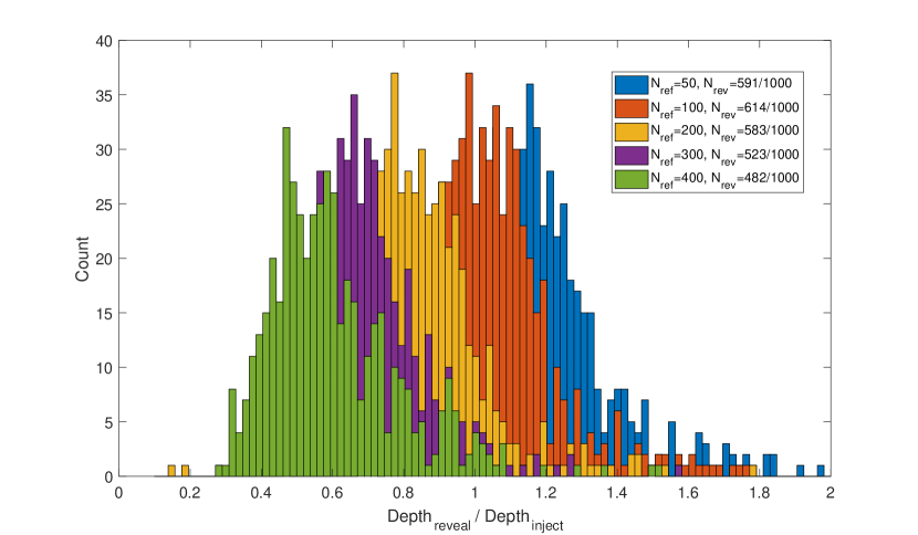
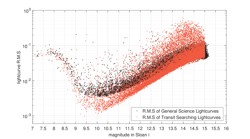
As with any other “blind-detrending” algorithm, the quality of our detrending procedure depends on the number of stars in the template. Although a larger number of template stars results in a lower RMS for the lightcurve, real transit signals may be suppressed to a strength below the detection threshold of our pipeline. Furthermore, large dips caused by eclipsing binaries may be reduced in amplitude to a level where they mimic planetary transits, thereby increasing false-positive rate. To find the optimal number of template stars, we ran a series of tests on a number of lightcurves with injected transit signals. We selected 1000 raw lightcurves from our original dataset and injected modeled transit signals into each of them. The radius of the host star was fixed to $1R_{\odot}$ , while the radius and period of the transiting planet were randomly selected in the range 0.25–2.0 $R_{\text{J}}$ and 0.1–7.0 days, respectively. Raw lightcurves with injected transits were then detrended and processed by our pipeline to find transit signals. Periods of all revealed signals were compared with the injected periods to remove any false detections. Figure 5 shows the distribution of the revealed number of transits versus the signal suppression ratio, ${\text{Depth}}_{\text{reveal}}/{\text{Depth}}_{\text{inject}}$ . Five numbers of reference stars in the template were tested: $N_{\text{ref}}=50$ , 100, 200, 300, 400. When the number of template stars was small, systematic errors were not removed effectively. Injected transit signals may be distorted by the remaining systematics and lead to a suppression ratio $\geq 1$ . When we increase the number of template stars, the suppression ratio decreases and its median goes well below unity. The total number of revealed signals also decreases with increasing $N_{\text{ref}}$ and the optimum value is around $N_{\text{ref}}=100$ . By adopting this $N_{\text{ref}}$ , we have achieved a photometric precision of $\sim$ 2.0 mmag around $m_{\textit{i}}=10.0$ and $\leq$ 10.0 mmag for stars brighter than $m_{\textit{i}}=12.5$ (see Figure 6). It is marginally enough to reveal a Jupiter-size exoplanet around a Solar-type star or an exo-Neptune around an M-dwarf. To go down below 1.0 mmag precision is quite difficult for us. The major drawbacks are the uncertainties within the flat-field correction and the intra/inter-pixel variations raised by the unperfect tracking operation that is caused by the frosting problem at Dome A. They are basically the same issue—if we could either fix the same stars on the same pixels all the time, or make a perfect flat-field, then the photometric precision will be improved significantly and allow us to detect smaller exoplanet. Unfortunately, none of them are an easy task at the Dome A, Antarctica. The good news is, as the number of sky images we acquired grows, we will be able to make better flat-fields in the future data releases.

4.2 Transit Signal Searching Module

The transit signals within a lightcurve can be modeled as a series of box-shape dips that show up periodically. One of the most effective ways to reveal this kind of signal is the BLS (Box-function Least Square Fitting) algorithm (Kovács et al., 2002). Our transit signal searching module is based on this well-tested method with some adjustments. The whole module can be divided into the following steps:

1.

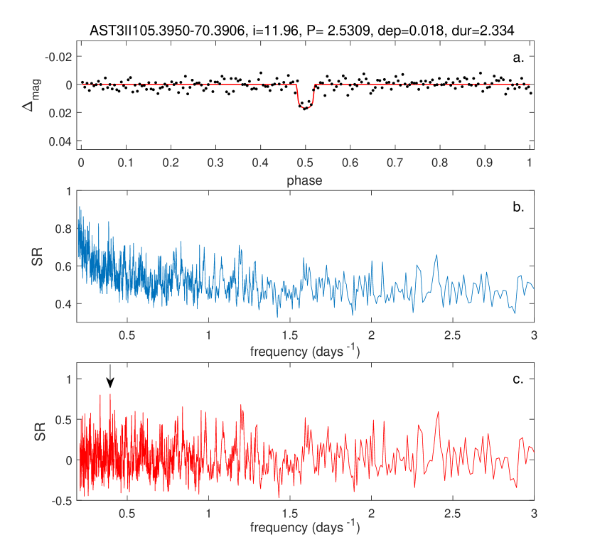
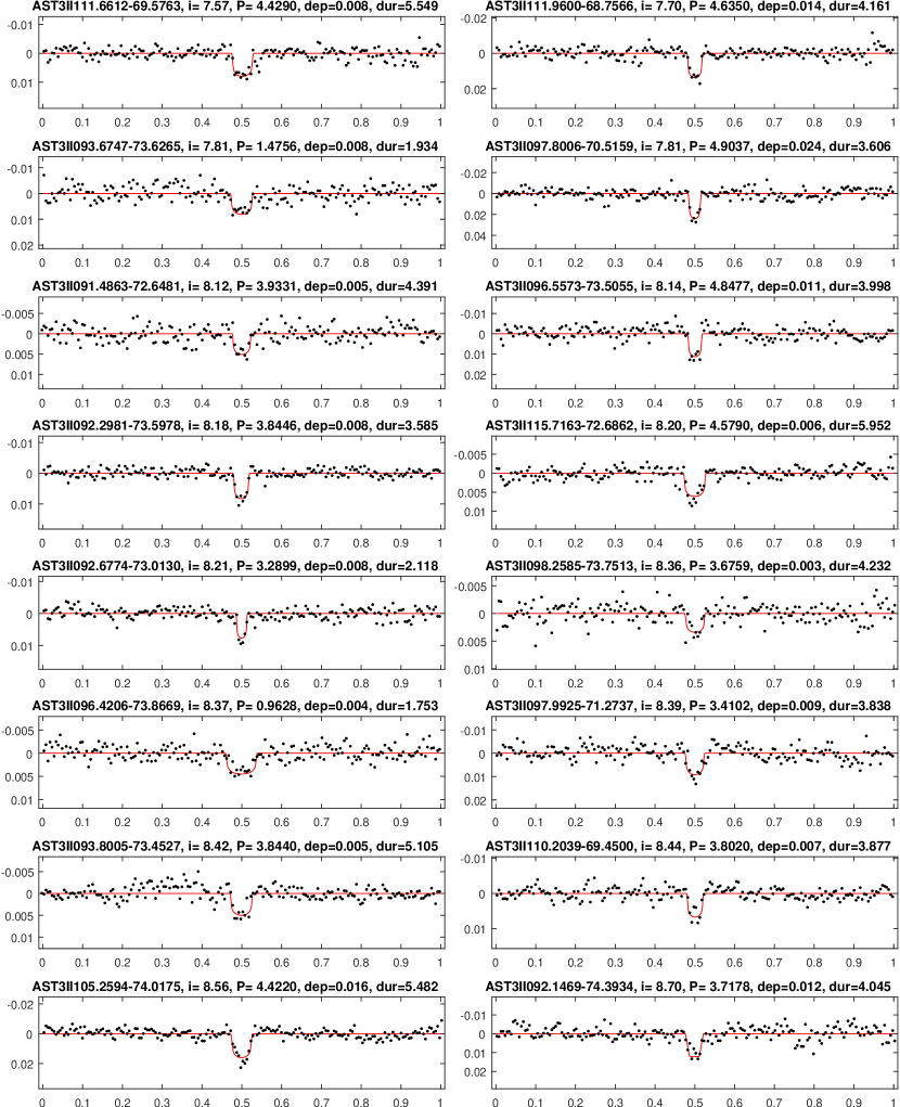
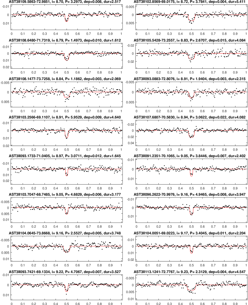
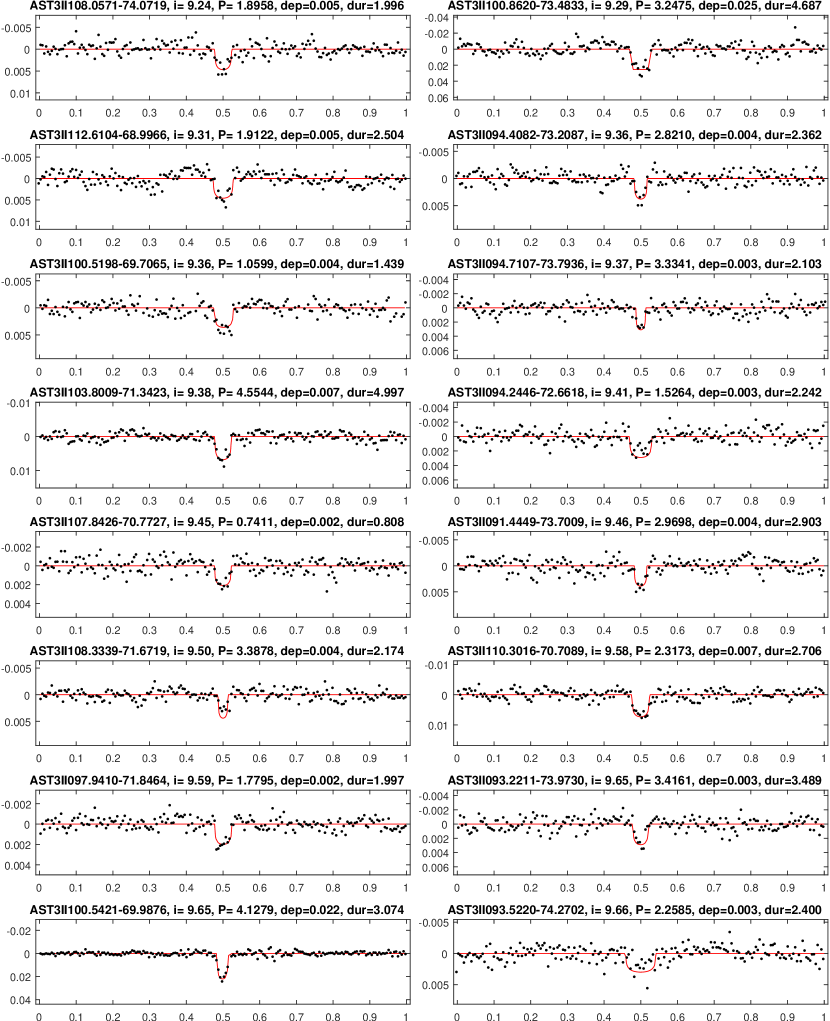
Pre-search by BLS fitting: the purpose of the first BLS run is to generate the frequency spectrum for each lightcurve. The range of periods $P$ and the fractional transit length $q$ are set to be wide enough to enclose as many potential transit signals as possible: $0.2\leq P\leq 10.0$ and $0.025\leq q\leq 0.25$ . The period resolution is set to be four times smaller than the sampling interval, which results in $\sim 2000$ steps in period. At each period step, the lightcurve is folded and binned to 200 phase bins before a box-function is fitted to it. The resulting SR (Signal Residue Kovács et al., 2002) periodogram is then subtracted using a moving median filter to remove the background trend caused by low-frequency systematic errors present in the lightcurve (Bakos et al., 2004; Wang et al., 2014). Figure 7 shows an example of the candidate “AST3II105.3950 $-$ 70.3906” whose signal is revealed after the periodogram detrending. We further calculate the SDE (Signal Detection Efficiency, Alcock et al., 2000; Kovács et al., 2002) for each peak identified from this detrended spectrum. Finally, we reject all peaks with $\mbox{SDE}<1.5$ and those peaks with periods very close to integer days (e.g., $\sim 1.0\pm 0.01$ days).
2.

BLS fitting over a refined period range: the first BLS run results in numerous candidate signals for each lightcurve. The second BLS run is to refine the parameters of signals found by the first run and filter out invalid ones. For each signal passing the first step, we perform a second BLS search in a narrow range of the earlier found period: $0.95P-1.05P$ . The period sampling number is fixed at 2000. Only the strongest signal within this period range is selected and delivered to the next step, provided the following criteria are matched: $\&N_{\text{tr}}\geq 3$ , $\Delta_{mag}\leq 0.05$ and $\mbox{SPN}\geq 6.0$ , where $N_{\text{tr}}$ is the number of transit dips, $\Delta_{mag}$ is the transit depth, and SPN is the Signal-to-Pink Noise ratio of the signal in the frequency spectrum. From the known statistics of exoplanets, the transit depths of confirmed planets are rarely greater than $5\%$ , so it is safe to restrict the range of depths to below $0.05$ ; larger depths are likely to be eclipsing binaries.
3.

Further detrending by TFA with signal-reconstruction: as mentioned above, our lightcurve detrending module may cause some signal suppression due to over-fitting. So, when an interesting signal is revealed by the previous steps, we perform an additional detrending process to the target lightcurve with the signal-reconstructive mode. This is done by using the “-TFA_SR” command in the VARTOOLS environment with the signals found by the last BLS refinement. Note that some lightcurves may contain multiple strong signals and they will be copied and detrended multiple times with the corresponding signals. This process will further reduce the RMS of the target lightcurve and enhance the strength of the target signal.
4.

Parameter filtering: the last step is to run BLS on each newly detrended lightcurve with a fixed period found in step 2, since the parameters of the transit signal may be changed after the TFA process with signal-reconstructive mode. The final transit signal is then filtered according to the following criteria: $\mbox{SNR}>3$ , $0.001<\Delta_{mag}<0.05$ and $0.5<T_{\text{dur}}<12$ , where SNR is the signal-noise ratio of the transit signal, and $T_{\text{dur}}$ is the transit duration in hours ,which are fitted by the BLS method.

After running all our data through the above steps (Figure 8), 1120 transit candidates (TCs) were found. This number of potential candidates is too high for easy visual inspection, so we designed a “Transit Signal Validation Module”, described in the next section, to assist.

4.3 Transit Signal Validation Module

Wide-field transiting exoplanet surveys tend to suffer from a high false-positive rate, especially when the photometric precision is marginally adequate to detect transit signals. Besides systematic errors, some true astrophysical variabilities, e.g., low-mass eclipsing binaries, grazing binaries and blended background binaries, may also mimic true transit signals. Therefore, effective validation procedures must be performed before further follow-up observations. A series of validation methods have been adopted in previous successful ground-based wide-field surveys such as WASP/SuperWASP (Pollacco et al., 2006), HATNET (Bakos et al., 2004) , HATSouth (Bakos et al., 2013), KELT (Pepper et al., 2007), OGLE (Udalski et al., 2002), and TrES (Alonso et al., 2004). Some key methods have been integrated into our validation module and proved to be effective in our previous work (Wang et al., 2014). In this section we present a similar version with some adjustments for the characteristics of the AST3-II data.

Our validation module (Figure 8) includes quantitative analysis and visual inspections as follows:

1.

Primary and secondary eclipses check: detached eclipsing binaries are one of the major sources of false alarms in many transiting exoplanet surveys. The reason is that an eclipsing low-mass star and a transiting planet will produce similar Box-shape signals, which are almost indistinguishable using the BLS method. The transit depth tells us about the secondary-to-primary radius ratio, $R_{\text{p}}/R_{\ast}$ . According to the statistics of confirmed exoplanets, transiting exoplanet with transit depths $\Delta_{mag}>0.05$ are very rare. So we may safely filter out some eclipsing binaries with very large transit depths in the previous filtering module. However, low transit depths may also be caused by a dwarf star transiting a giant or super giant host. Detecting such objects requires using other features of the light curve. Other than the transit depth, one major difference between an eclipsing binary and a transiting exoplanet is the secondary eclipse that occurs when the secondary star or the planet is blocked by the host star. Since a planet does not self-illuminate, the depth of its secondary eclipse will be much shallower than that of an eclipsing binary. So our first step is to check the existence of any secondary eclipse within a candidate lightcurve. We phase fold the lightcurve and fix the primary eclipse at phase 0.5, according to the detected period. Then we subtract the fitted model given from the BLS fitting and calculate the RMS of the residuals at phases around 0.0 and 0.5. Since the model will only fit the primary eclipse, if a secondary eclipse exists, the RMS at phase 0.0 will be significantly greater than the RMS at phase 0.5. Any candidate with $\mbox{RMS}_{\text{phase}=0.0}/\mbox{RMS}_{\text{phase}=0.5}>2.0$ is labeled as suspect and requires visual inspection. For each candidate that passes the above procedure, we further estimate the statistical difference between the odd and even transits, and use the significance level of the consistency in transit depth, $P_{\Delta}$ , to determine whether the odd and even transits are drawn from the same population (Wu et al., 2010). The smaller this statistic is, the more inconsistent the odd and even transits are, and the more likely the event is a false positive. The acceptance boundary is set to be 0.05 and we rejected 355 candidates with $P_{\Delta}<0.05$ .
2.

Aperture blending check: a blended eclipsing binary is another major source of mimics for genuine transiting planet signals in wide-field surveys. The pixel-scale of AST3-II is $\sim 1^{\prime\prime}$ pixel^-1, so it is unlikely that more than one bright star will fall into a single pixel. However, to avoid saturating bright stars, we defocus the optics slightly to have a FWHM $\sim 5$ pixels and employ three photometric apertures: 8, 10 and 12 pixels (Zhang et al., 2018). When the target field is too crowded with stars, it is likely that there will be background stellar objects within the photometric apertures of the target star. And the target star could also be contaminated by scattered light from nearby bright stars. If the contaminating star or the target star itself is in fact an eclipsing binary, its eclipsing depth will be diluted, making it look like a planetary transit. In this case, the secondary eclipse will also be made shallower, to a level that may be undetectable by our precision. So we perform a further blending check on those candidates that passed the first step. To do this we cut a stamp from the image with a size of $150\times 150$ pixels for each candidate and check for blending or contaminating objects by human inspections. Since the angular resolution of AST3-II is reasonably high, this procedure is quite accurate and efficient, and 180 candidates with suspicious blending events were rejected.
3.

Sinusoidal variation check: besides low-depth eclipses caused by binaries, some brightness variations can be caused by systematic errors or intrinsic stellar variability with a time scale similar to the planetary transit—the dimming part of the variation is easily mistaken as a dip caused by a planetary transit when we fit the phase-folded lightcurve with a box-shape function. However, measurements caused by systematics or the intrinsic stellar variability are often strongly correlated. And in such a lightcurve, the dimming and brightening parts should show up periodically, typically with a sinusoidal variation. A phase-folded lightcurve with a genuine transit event will result in only one obvious transit (dimming) detection without any strong anti-transit (brightening) detection. In this step, we calculate the ratio of improvements for the best-fit transit (dimming), $\Delta\chi_{-}^{2}$ , to the improvements for the best-fit anti-transit (brightening), $\Delta\chi_{+}^{2}$ , for each lightcurve. This measurement provides an estimate of whether a detection has the expected properties of a credible transit signal, rather than the properties of the systematic error or intrinsic stellar sinusoidal variability (Burke et al., 2006). At the end of this step 320 candidates with $\Delta\chi_{-}^{2}/\Delta\chi_{+}^{2}<1.5$ were rejected.
4.

Transit shape check: a plausible transit shape is one of the most important criteria to validate a good transit candidate. Since the checks above have reduced the number of potential candidates to a level where visual inspection by human eyes is feasible, we checked each candidate independently by two authors (Dr. Zhouyi Yu and Dr. Ming Yang) with the same criteria: I. a complete transit dip with both the ingress and egress parts present; II. two flat “shoulders” before and after the transit; III. a smooth phase coverage without too many gaps. Candidates were labeled as “bad target” if they showed clear evidence of variability out of transit, including a secondary eclipse, an ellipsoidal variation, or a realistic variability of other forms. If both human inspectors labeled the same candidate as “bad target”, this candidate was removed. At the end of this stage, the number of remaining candidates was reduced to 243.

Transit model fit: during this stage we perform theoretical model fits to each remaining candidate. The aim is to determine some key parameters of the transit event and filter out inconsistent systems. Before the transit model fit, we calculate the SRN (the Signal-to-Red Noise ratio) of each lightcurve. Besides the uncorrelated white noise, the errors of bright stars in ground-based wide-field photometric surveys are usually dominated by correlated red noise (Pont et al. 2006). Therefore, SRN is a simple and robust parameter to assess the significance of the detected transit event:

\text{SRN}=\frac{d}{\sigma_{\text{r}}}\sqrt{N_{\text{tr}}},

(3)

where $d$ is the best-fitting transit depth, $\sigma_{\text{r}}$ is the uncertainty of the transit depth in the presence of red noise and $N_{\text{tr}}$ is the number of observed transit dips. The simplest way of assessing the level of red noise ( $\sigma_{\text{r}}$ ) present in the data is to compute a sliding average of the out-of-transit data over the $n$ data points contained in a transit-length interval. This method was proposed by Pont et al. (2006) and has been successfully applied to the SuperWASP candidates (Christian et al., 2006; Clarkson et al., 2007; Kane et al., 2008; Lister et al., 2007; Street et al., 2007). Pont et al. (2006) suggests a typical threshold range of $\mbox{SRN}\sim 7$ –9 based on a red noise level of $\sigma_{r}\sim 3.0$ mmag. The typical value of $\sigma_{\text{r}}$ present in the AST3-II lightcurves of bright stars is $2.3$ mmag and we find that some candidates with $\mbox{SRN}\sim 5$ look plausible. To avoid missing some interesting systems, we saved all candidates with $\mbox{SRN}\geq 5$ . This threshold filters out 21 candidates and passes 222 candidates.

The remaining 222 lightcurves are then modeled using the Mandel-Agol algorithm (Mandel & Agol, 2002) integrated in VARTOOLS (Hartman & Bakos, 2016). The fitted parameters of these candidates, such as period( $P$ ), epoch, planet-to-star radius ratio ( $R_{\text{p}}/R_{\ast}$ ), semi-major axis ( $a_{\text{p}}/R_{\ast}$ ) and inclination ( $i$ ) of planet’s orbit are listed in Table 2. We also calculate the ratio of the observed duration to the theoretical duration ( $\eta$ ). This is another quantitative parameter that can be used as a filter, based on the theoretical model of the transit method. If a transit event is caused by a real planet, its transit duration, $T_{\text{dur}}$ measured directly from the phase-folded lightcurve, should be close to the theoretical duration, $T_{\text{theory}}$ , calculated from the fitted parameters. This means that if $\eta\equiv T_{\text{dur}}/T_{\text{theory}}\approx 1$ , the exoplanet candidate is expected to have a high probability of being a real planet. Here we employ an approximation to $T_{\text{theory}}$ :

T_{\text{theory}}=\frac{P}{\pi}\arcsin\left(\frac{\sqrt{(1+R_{\text{p}}/R_{\ast})^{2}-(a/R_{\ast})^{2}cos^{2}i}}{a/R_{\ast}}\right),

(4)

where $P$ is the measured period of the transit signal, $R_{\text{p}}$ is the fitted planet radius, $a$ is the fitted orbital semi-major axis, $i$ is the fitted inclination of planet’s orbit, and $R_{\ast}$ is the fitted radius of the central star. This criterion was first introduced by Tingley & Sackett (2005) in checking for candidates found by OGLE, and has been successfully applied to many WASP candidates. For each candidate, we provide $\eta$ in the 11th column of Table 2 and most of our candidates have a value close to unity.

6.

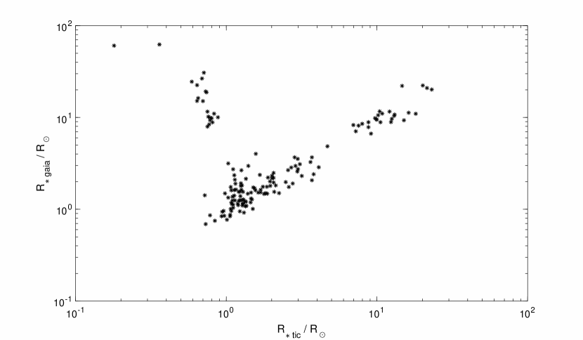
Stellar properties check: the last step is to check the stellar radius to eliminate giant stars. For each candidate, we calculate three radii, $R_{\text{p}}^{\text{tic}}$ , $R_{\text{p}}^{\text{gaia}}$ and $R_{\text{p}}^{\text{hem}}$ , according to the transit depth and the stellar radii from the TIC (TESS Input Catalog, Stassun et al., 2017) , Gaia DR2 (Gaia Collaboration et al., 2018) and TESS-HERMES (Sharma et al., 2018) catalogs. We set a critical radius, $R_{\text{crit}}=2R_{\text{J}}$ , to distinguish giant planets from stellar objects. If $R_{\text{p}}^{\text{tic}}\leq R_{\text{crit}}$ and $R_{\text{p}}^{\text{gaia}}\leq R_{\text{crit}}$ , this candidate is labeled as a “TC” (Transit Candidate). If both $R_{\text{p}}^{\text{tic}}$ and $R_{\text{p}}^{\text{gaia}}$ are greater than $R_{\text{crit}}$ , this candidate is removed and labeled as a “LB” (Low depth eclipsing Binary). We notice that many stellar radii from TIC and Gaia are not consistent, especially for dwarf stars in the TIC catalog—they are often labeled as giants in the Gaia DR2 catalog (see Figure 9). When $R_{\text{p}}^{\text{tic}}$ and $R_{\text{p}}^{\text{gaia}}$ are not consistent, e.g, $R_{\text{p}}^{\text{tic}}\leq R_{\text{crit}}$ and $R_{\text{p}}^{\text{gaia}}>R_{\text{crit}}$ , this candidate is labeled by a tag of “TC?” which means further inspection of the stellar properties is required. If both $R_{\text{p}}^{\text{tic}}$ and $R_{\text{p}}^{\text{gaia}}$ are not available, we use $R_{\text{p}}^{\text{hem}}$ as a reference. Finally, if no stellar radius is available, these candidates are also labeled “TC?”. For easy retrieval, this these transit tags are listed in both Table 2 and Table 3.

At the end of this validation module, we have 116 transiting exoplanet candidates remaining: 72 of them are strong candidates and further inspections are required for the other 44 candidates. Detailed information for all 116 candidates is listed in Table 3.

5 Results

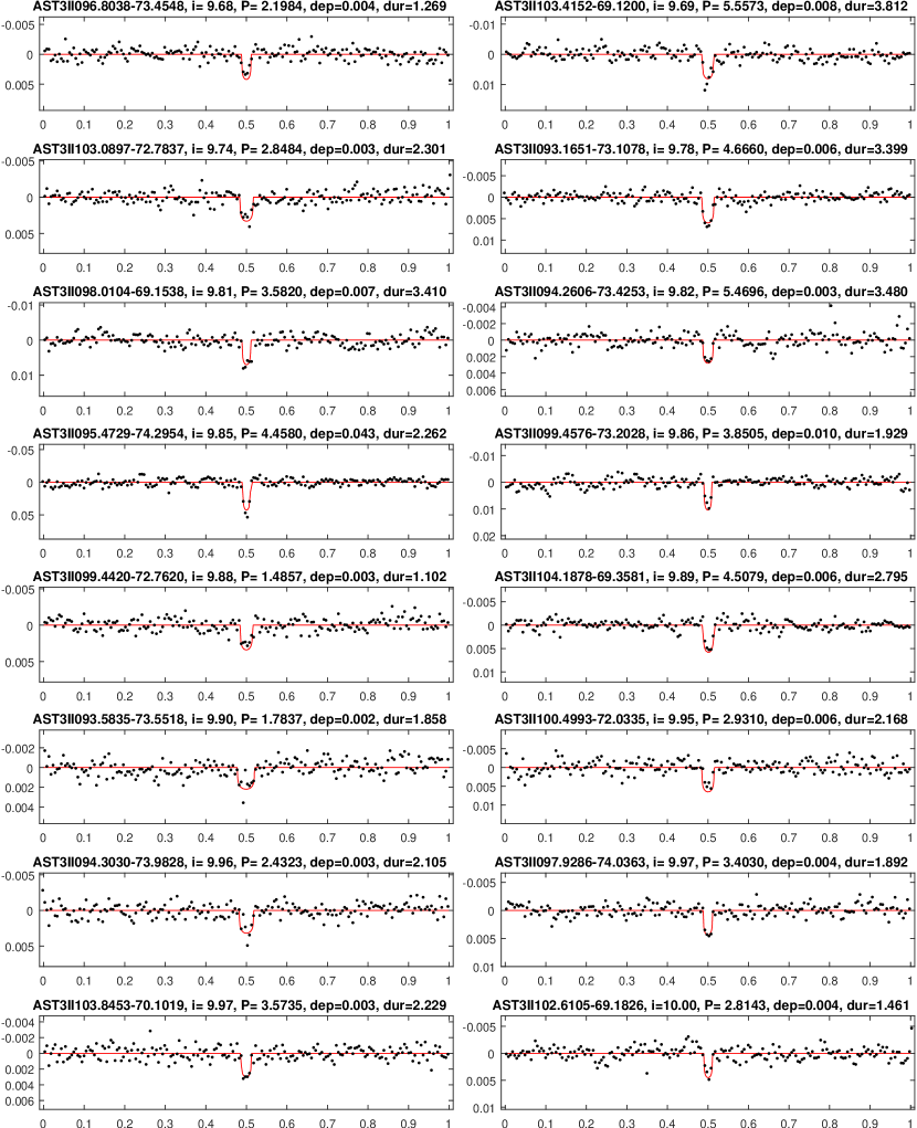
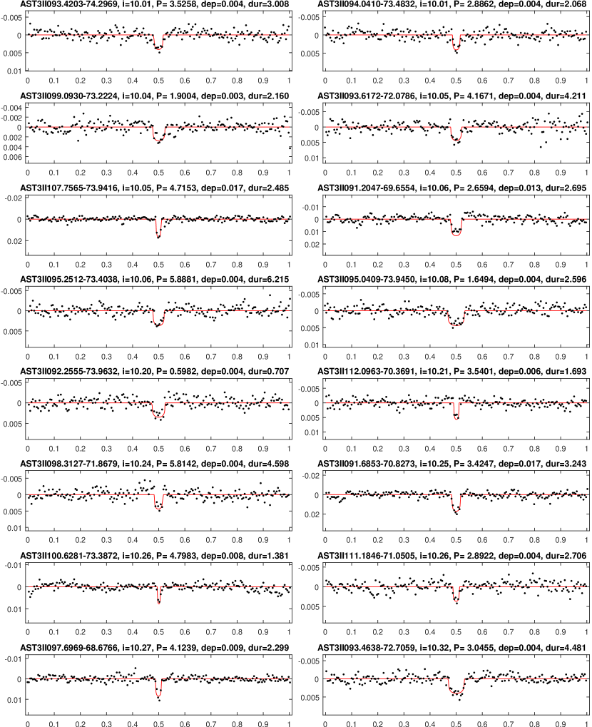
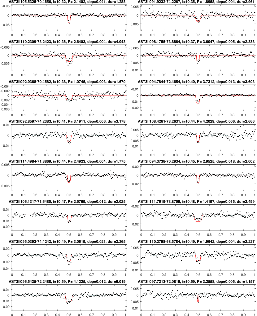
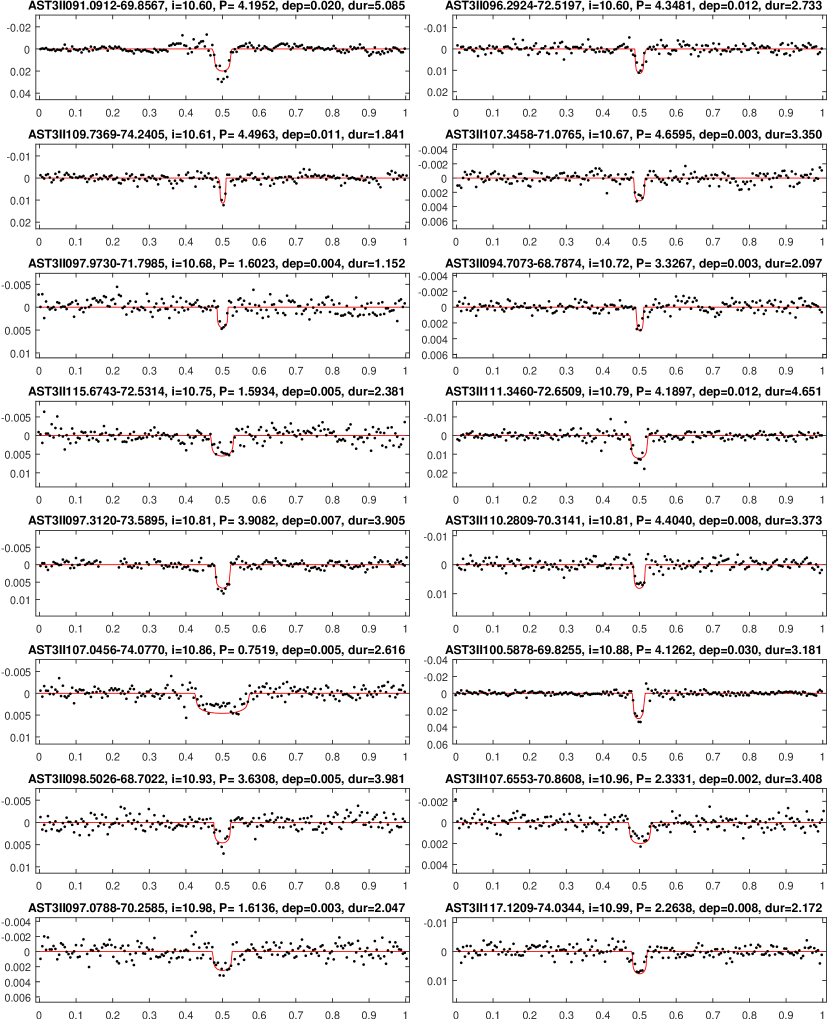
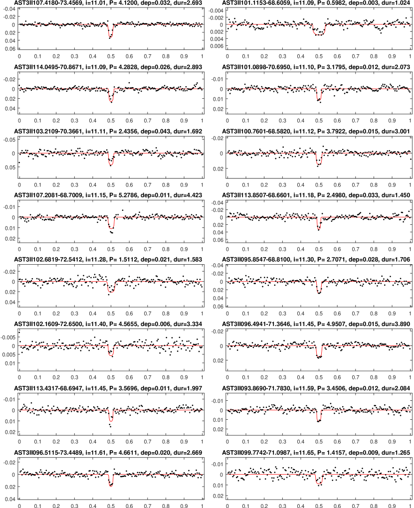
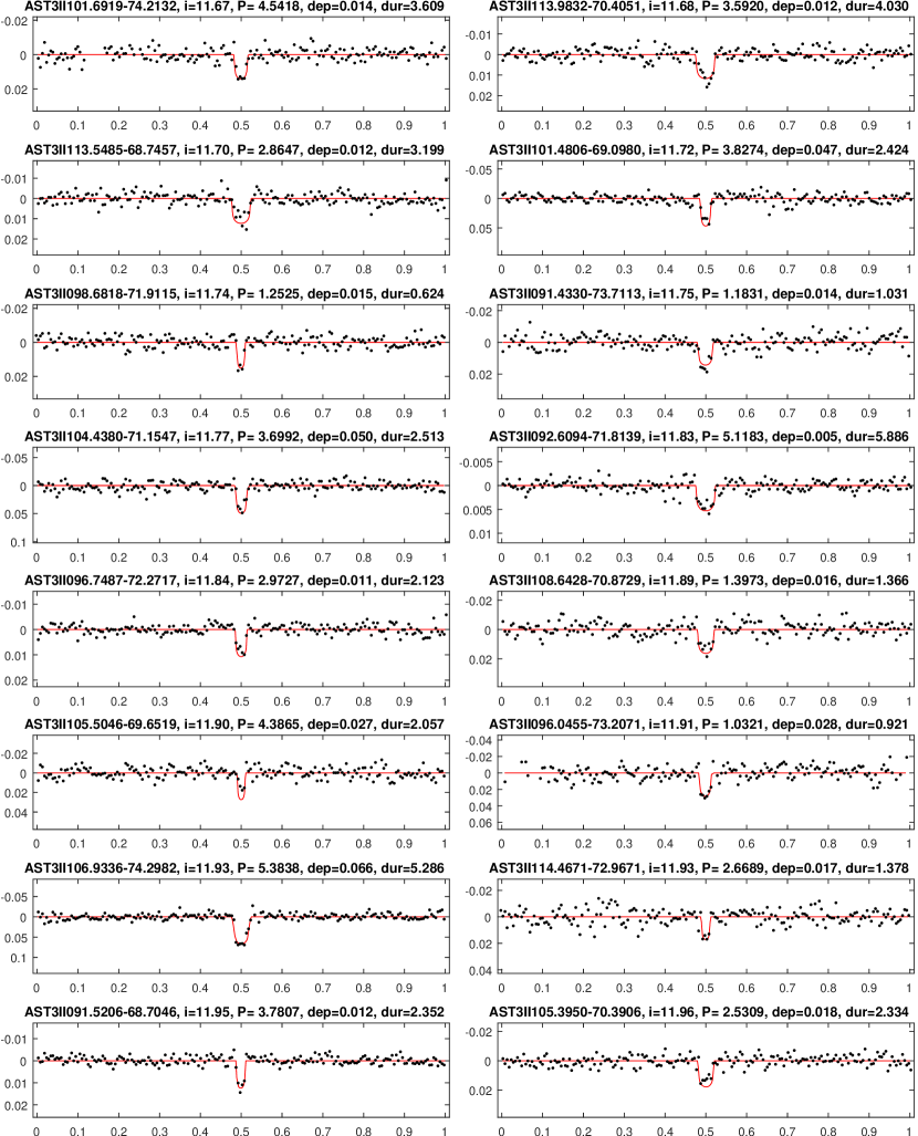
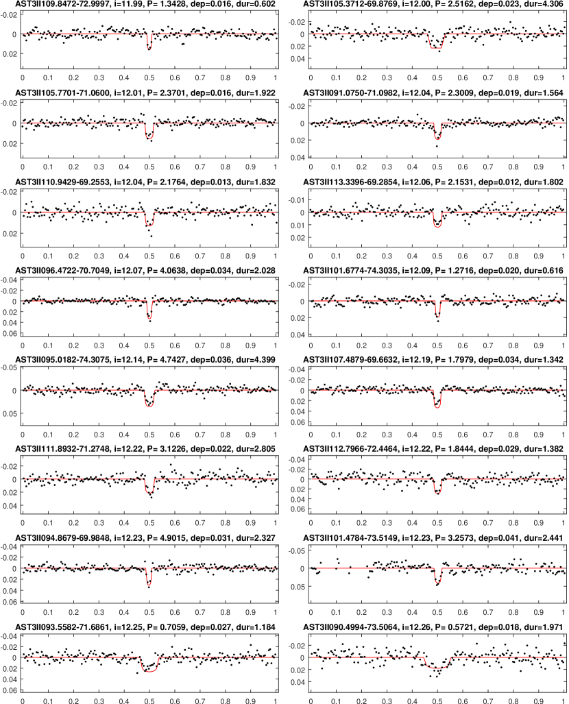
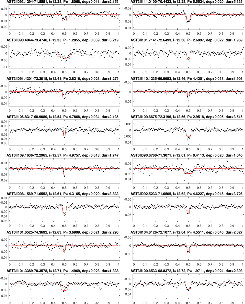
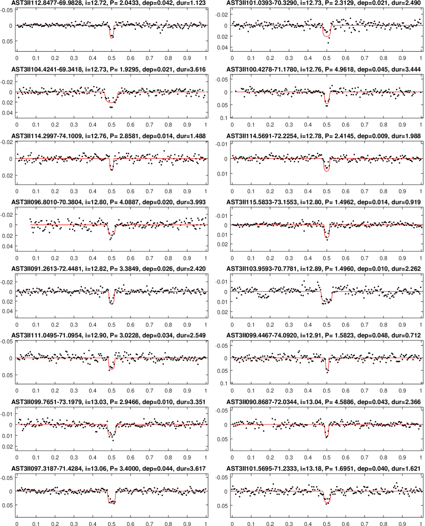
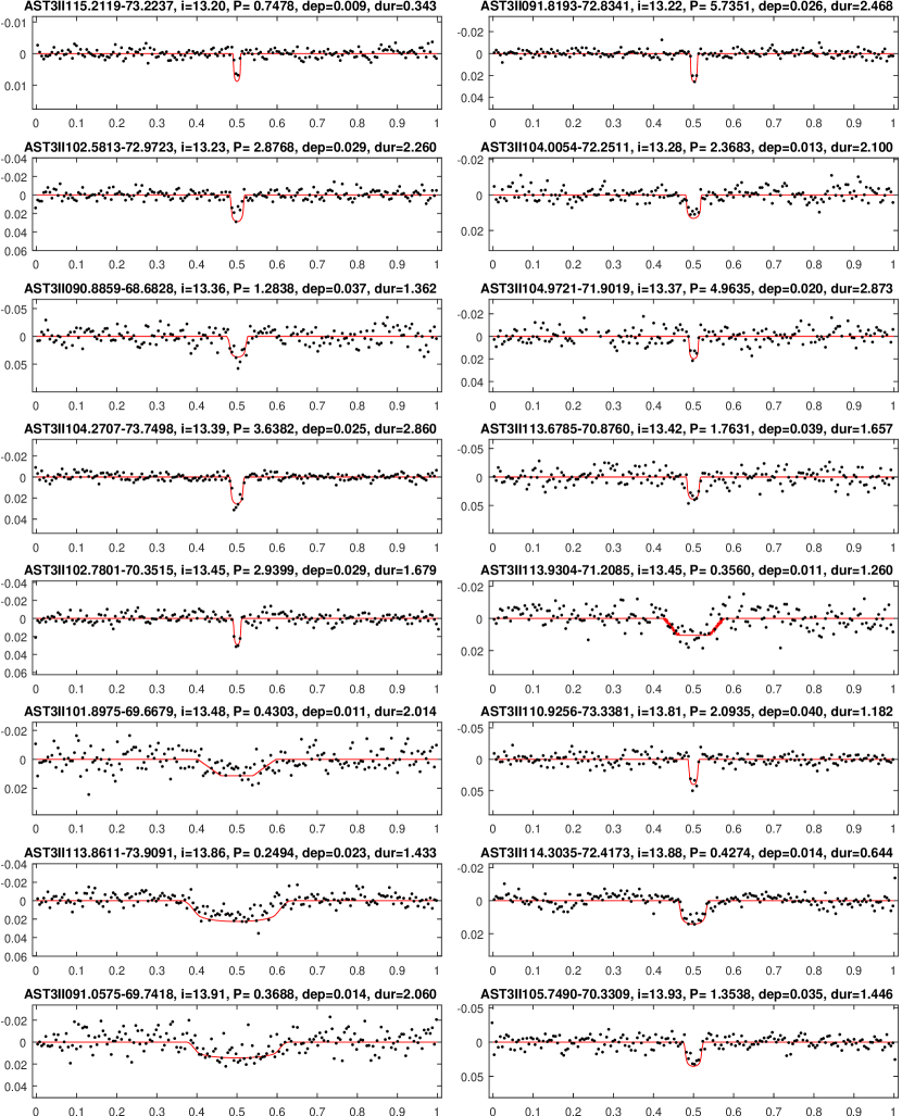
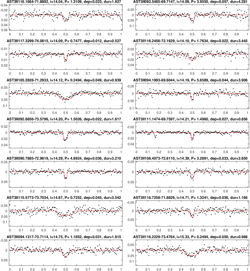
Our transit signal searching and validation modules have revealed a total of 222 plausible transit events. The transit signals were fitted by a Mandel-Agol model, and all the fitted parameters, including the transit epoch, period, depth, and duration, are listed in Table 2. Lightcurves for all 222 targets are shown in Figure 10–23. Each lightcurve has been folded to the fitted period and binned to 200 bins. The red solid line denotes the best-fit model for each phase-folded transit. All targets are cross-matched with the newly released TIC (Stassun et al., 2017), Gaia DR2 (Gaia Collaboration et al., 2018), and TESS-HERMES (Sharma et al., 2018) catalogs to obtain the stellar properties (such as radius) of their host stars. The planetary radius of each transit candidate is then derived according to the fitted value of $R_{\text{p}}/R_{\ast}$ . The stellar properties of the host stars are listed in Table 3. A tag is assigned to each target: “TC”, “LB” or “TC?”, which mean strong “Transit Candidate”, “Low-depth Binary” and “Transit Candidate but further inspections are required”, respectively. Of the 116 transiting exoplanet candidates found, 72 are strong candidates (“TC”) and 44 need further checks on their host radii (“TC?”). The smallest transit signal revealed in this work is around $\Delta_{mag}\sim 2$ mmag (e.g., target AST3II107.8426 $-$ 70.7727, AST3II093.5835 $-$ 73.5518 and AST3II107.6553 $-$ 70.8608) and the longest period is around $P\leq 6.0$ days (e.g., AST3II103.2566 $-$ 69.1107), which shows the promising capability of AST3 telescopes to find small-radius short-period transiting planets in the high-declination Antarctic sky. Raw and detrended Lightcurves of these targets and other stars are available to the community through the website of the School of Astronomy and Space Science, Nanjing University ¹¹1http://www.njutido.com/tido/data.html or http://116.62.78.33/tido/data.html and the Chinese Astronomical Data Center ²²2http://casdc.china-vo.org/archive/ast3/II/dr1/.

6 Summary and Conclusions

AST3-II is a 50 cm telescope located at Dome A (the highest point of Antarctica) enabling near-continuous observations in the i-band during the Antarctic polar nights. It is designed to withstand the harsh climatic conditions at Dome A and has been used to perform a wide-field (FoV $\approx 1.5^{\circ}\times 3^{\circ}$ ) and high-resolution ( $\approx 1.0^{\prime\prime}$ pixel^-1) photometric survey with a photometric precision of several millimagnitudes. Using the AST3 telescopes, the CHESPA (CHinese Exoplanet Searching Program from Antarctica) survey has been running since 2012, and 48 target fields within the Southern CVZ of TESS were scheduled to be surveyed between 2016 and 2019. During the austral winters of 2016 and 2017, the AST3-II telescope has successfully scanned 32 target fields.

Data from the first 10 target fields surveyed in 2016 have been fully reduced and released by Zhang et al. (2018). We have achieved a precision (RMS of the entire lightcurve) of $<2$ mmag at $\textbf{{m}}_{\textit{i},\text{apass}}\approx 10$ mag and $\sim 50$ mmag at $\textbf{{m}}_{\textit{i},\text{apass}}\approx 15$ mag with a cadence of 36 minutes (Figure 6). In this work, we describe our lightcurve detrending, transit signal searching and validation modules in detail and present a catalog of 222 plausible transit signals. When combined with the stellar information given by the TIC, Gaia DR2 and TESS-HERMES catalogs, 116 targets are labeled as transit candidates, of which 72 targets are strong candidates and 44 candidates require further inspections of the stellar parameters of their hosts. The other 106 targets are ruled out because their derived planetary radii are too large, i.e., $R_{p}>2R_{\text{Jupiter}}$ . Almost all of our new exoplanet candidates are listed in the input catalog of the TESS project and some are on the high priority list (CTL). Therefore high precision photometric follow-up from TESS will be available soon after the TESS data release in late 2018. We are now working on obtaining radial velocity observations of our candidates to confirm them using the new Veloce facility on the 3.9m Anglo-Australian Telescope (Gilbert et al., 2018), and MINERVA-Australis facility (Wittenmyer et al., 2018). The results of these follow-up observations will be presented in forthcoming papers.

TESS was launched successfully in 2018 April and will map most bright stars within the southern hemisphere. Thousands of small exoplanet candidates orbiting bright nearby stars are expected to be revealed in the coming couple of years and follow-up observations with high angular resolution or different wavelengths are required. AST3-II is the first wide-field survey telescope to have worked through the long polar nights at the top of the Antarctica plateau, without any human attendance on-site during the observation campaigns. Our results demonstrate the high potential of the AST3 telescopes at Dome A to perform accurate and continuous wide-field photometric surveys. With the advantages of the polar site, the AST3 telescopes could continuously monitor hundreds of thousands of target stars around the South Ecliptic Pole for months without substantial interruption. This is particularly important for performing cross-validations of transit candidates found by TESS. We believe our catalog of new transit candidates within the Southern CVZ of TESS will be a helpful reference for the flood of new candidates soon to emerge from TESS.

This work was supported by the Natural Science Foundation of China (NSFC grants 11673011, 11333002, 11273019), National Basic Research Program (973 Program) of China (Grant Nos. 2013CB834900, 2013CB834904). The authors deeply appreciate all the CHINAREs for their great effort in installing/maintaining CSTAR, CSTAR-II, AST3-I, AST3-II and PLATO-A. This study has also been supported by the Chinese Polar Environment Comprehensive Investigation & Assessment Program (Grant No. CHINARE2016-02-03), the Australian Antarctic Division, and the Australian National Collaborative Research Infrastructure Strategy administered by Astronomy Australia Limited. Zhang is also grateful to the High Performance Computing Center (HPCC) of Nanjing University for reducing the data used in this paper. .

Appendix A Appendix Data

Table 2: Fitted parameters of Exoplanet candidates from AST3-II observations in 2016

Target ID^a^aIDs of AST3-II targets in the format “AST3II $+$ RA $+$ Dec’.	i ${}_{\text{apass}}$ ^b^bi_apass: i-band magnitudes from the APASS catalog.	Epoch	$P$ ^c^c $P$ : the observed period of the transit signal.	$\Delta_{mag}$ ^d^d $\Delta_{mag}$ : the transit depth in Sloan i-band magnitude.	$T_{\text{dur}}$ ^e^e $T_{\text{dur}}$ : the observed transit duration.	SRN^f^fSRN: the Signal-to-Red-Noise-Ratio of the transit event.	$R_{\text{p}}/R_{\ast}$ ^g^g $R_{\text{p}}/R_{\ast}$ : the planet’s fitted radius as a fraction of the host star radius. The fit is based the model given by Mandel & Agol (2002).	$a/R_{\ast}$ ^h^h $a/R_{\ast}$ : the fitted semi-major axis of planet’s orbit in the unit of its host star radius.	$i$ ⁱⁱ $i$ : The fitted orbital inclination relative to the line-of-sight of observer.	$\eta$ ^j^j $\eta$ : The ratio of the observed transit duration to the theoretical duration: $\eta=T_{\text{dur}}/T_{\text{theory}}$ .	tag^k^kLabels from AST3-II observation: “TC”, Transit Candidate; “TC?”, Transit Candidate but needs further inspection; “LB”, Low-depth Binary.
AST3II $+$	mag	JD2456000 $+$	[day]	[mag]	[hour]	$-$	$-$	$-$	[degree]	$-$	$-$
AST3II111.6612 $-$ 69.5763	7.57	1524.843179	4.4290	0.008	5.549	8.5	0.083	6.342	89.61	0.96	$TC?$
AST3II111.9600 $-$ 68.7566	7.70	1526.252284	4.6350	0.014	4.161	7.0	0.116	8.878	89.84	0.93	$LB$
AST3II093.6747 $-$ 73.6265	7.81	1513.297757	1.4756	0.008	1.934	5.9	0.086	6.088	89.66	0.96	$TC?$
AST3II097.8006 $-$ 70.5159	7.81	1513.325399	4.9037	0.024	3.606	10.2	0.144	10.860	89.77	0.91	$LB$
AST3II091.4863 $-$ 72.6481	8.12	1513.100016	3.9331	0.005	4.391	6.2	0.070	7.194	89.85	0.98	$LB$
AST3II096.5573 $-$ 73.5055	8.14	1514.770168	4.8477	0.011	3.998	5.9	0.104	9.538	89.77	0.93	$TC?$
AST3II092.2981 $-$ 73.5978	8.18	1513.507046	3.8446	0.008	3.585	7.6	0.090	8.556	89.78	0.96	$TC?$
AST3II115.7163 $-$ 72.6862	8.20	1512.691684	4.5790	0.006	5.952	7.6	0.077	6.127	89.78	0.96	$LB$
AST3II092.6774 $-$ 73.0130	8.21	1515.241308	3.2899	0.008	2.118	7.1	0.086	12.274	89.85	0.95	$TC$
AST3II098.2585 $-$ 73.7513	8.36	1512.679419	3.6759	0.003	4.232	5.7	0.057	6.873	89.75	0.98	$TC$
AST3II096.4206 $-$ 73.8669	8.37	1512.646819	0.9628	0.004	1.753	6.3	0.067	4.293	89.66	0.95	$TC?$
AST3II097.9925 $-$ 71.2737	8.39	1512.951248	3.4102	0.009	3.838	5.9	0.095	7.050	89.87	0.94	$TC?$
AST3II093.8005 $-$ 73.4527	8.42	1513.553541	3.8440	0.005	5.105	7.0	0.070	6.032	89.65	0.98	$LB$
AST3II110.2039 $-$ 69.4500	8.44	1525.343785	3.8020	0.007	3.877	6.9	0.067	8.187	89.45	1.02	$LB$
AST3II105.2594 $-$ 74.0175	8.56	1516.017356	4.4220	0.016	5.482	7.2	0.124	6.475	89.79	0.93	$TC$
AST3II092.1469 $-$ 74.3934	8.70	1513.291485	3.7178	0.012	4.045	8.9	0.110	7.045	89.05	0.91	$TC?$
AST3II109.5863 $-$ 72.9851	8.70	1515.191356	3.2973	0.008	2.517	6.3	0.090	10.403	89.90	0.95	$LB$
AST3II102.8569 $-$ 69.0175	8.72	1513.699849	3.7841	0.004	5.411	7.7	0.062	5.192	89.60	0.91	$LB$
AST3II108.6480 $-$ 71.7319	8.79	1512.941901	1.4973	0.010	1.612	9.4	0.101	7.309	89.82	0.93	$LB$
AST3II105.5428 $-$ 73.2557	8.83	1513.283077	2.6707	0.015	4.084	9.9	0.119	5.192	89.66	0.92	$LB$
AST3II108.1477 $-$ 73.7258	8.84	1512.412260	1.1862	0.003	2.069	5.7	0.052	4.418	89.05	0.95	$LB$
AST3II093.0883 $-$ 72.8076	8.91	1513.826244	1.9404	0.003	2.315	6.9	0.052	6.634	89.76	0.98	$TC$
AST3II103.2566 $-$ 69.1107	8.91	1517.612826	5.9529	0.009	4.640	9.4	0.090	10.175	89.76	0.95	$LB$
AST3II107.6807 $-$ 70.5830	8.94	1513.486838	3.0622	0.022	4.082	13.3	0.148	5.974	89.72	0.90	$LB$
AST3II093.1733 $-$ 71.0405	8.97	1515.213181	3.0711	0.012	1.645	8.0	0.108	14.868	89.87	0.94	$LB$
AST3II091.2351 $-$ 70.1065	9.05	1513.830133	3.8446	0.007	2.402	7.8	0.086	12.561	89.83	0.95	$LB$
AST3II103.7047 $-$ 68.7485	9.05	1514.495588	4.6829	0.006	3.177	7.7	0.075	11.720	89.89	0.97	$TC?$
AST3II104.0645 $-$ 73.8668	9.16	1514.773768	2.5527	0.005	3.748	6.3	0.068	5.380	89.60	0.96	$LB$
AST3II096.2622 $-$ 70.9976	9.16	1513.910238	4.9465	0.008	3.947	7.0	0.085	9.984	89.72	0.96	$TC$
AST3II104.0051 $-$ 69.0223	9.17	1512.776310	3.4045	0.011	2.204	9.0	0.103	12.251	89.89	0.94	$TC$
AST3II093.7421 $-$ 69.1334	9.22	1516.106964	4.7067	0.007	3.527	8.6	0.065	11.054	89.61	1.02	$LB$
AST3II113.1241 $-$ 72.7767	9.23	1514.502942	2.3129	0.004	4.547	5.2	0.062	4.066	89.59	0.97	$TC?$
AST3II108.0571 $-$ 74.0719	9.24	1512.918276	1.8958	0.005	1.996	6.2	0.078	7.142	89.75	0.91	$LB$
AST3II100.8620 $-$ 73.4833	9.29	1529.721051	3.2475	0.025	4.687	7.8	0.159	5.325	89.05	0.86	$LB$
AST3II112.6104 $-$ 68.9966	9.31	1526.262433	1.9122	0.005	2.504	5.9	0.067	6.016	89.68	0.96	$TC$
AST3II100.5198 $-$ 69.7065	9.36	1526.023254	1.0599	0.004	1.439	8.0	0.054	6.165	89.63	1.04	$TC$
AST3II094.4082 $-$ 73.2087	9.36	1514.321763	2.8210	0.004	2.362	5.2	0.060	9.437	89.84	0.97	$LB$
AST3II094.7107 $-$ 73.7936	9.37	1513.455812	3.3341	0.003	2.103	5.7	0.056	12.413	89.81	0.97	$TC$
AST3II103.8009 $-$ 71.3423	9.38	1515.218426	4.5544	0.007	4.997	8.4	0.082	7.239	89.86	0.96	$LB$
AST3II094.2446 $-$ 72.6618	9.41	1512.530151	1.5264	0.003	2.242	8.6	0.054	5.366	89.83	0.97	$LB$
AST3II107.8426 $-$ 70.7727	9.45	1512.304499	0.7411	0.002	0.808	6.8	0.045	7.210	89.69	0.98	$TC$
AST3II091.4449 $-$ 73.7009	9.46	1515.049569	2.9698	0.004	2.903	6.9	0.045	9.537	89.42	1.17	$TC$
AST3II108.3339 $-$ 71.6719	9.50	1515.499350	3.3878	0.004	2.174	6.4	0.066	12.232	89.84	0.96	$LB$
AST3II110.3016 $-$ 70.7089	9.58	1525.988448	2.3173	0.007	2.706	6.7	0.085	6.861	89.80	0.96	$TC?$
AST3II097.9410 $-$ 71.8464	9.59	1513.311537	1.7795	0.002	1.997	8.2	0.044	7.104	89.80	1.00	$TC$
AST3II093.2211 $-$ 73.9730	9.65	1512.895397	3.4161	0.003	3.489	8.3	0.053	7.852	89.66	0.99	$LB$
AST3II100.5421 $-$ 69.9876	9.65	1514.764083	4.1279	0.022	3.074	9.3	0.144	10.591	89.84	0.90	$LB$
AST3II093.5220 $-$ 74.2702	9.66	1513.237956	2.2585	0.003	2.400	5.4	0.048	4.000	89.39	0.53	$TC?$
AST3II096.8038 $-$ 73.4548	9.68	1513.805829	2.1984	0.004	1.269	6.5	0.064	13.851	89.88	0.98	$TC?$
AST3II103.4152 $-$ 69.1200	9.69	1513.627225	5.5573	0.008	3.812	6.7	0.088	11.507	89.86	0.95	$TC?$
AST3II103.0897 $-$ 72.7837	9.74	1514.178510	2.8484	0.003	2.301	8.5	0.053	9.920	89.71	1.00	$LB$
AST3II093.1651 $-$ 73.1078	9.78	1516.196945	4.6660	0.006	3.399	6.8	0.073	10.939	89.75	0.97	$LB$
AST3II098.0104 $-$ 69.1538	9.81	1515.451792	3.5820	0.007	3.410	7.7	0.064	11.806	86.93	1.72	$LB$
AST3II094.2606 $-$ 73.4253	9.82	1513.359890	5.4696	0.003	3.480	6.7	0.052	12.530	89.85	0.99	$TC$
AST3II095.4729 $-$ 74.2954	9.85	1526.661107	4.4580	0.043	2.262	6.4	0.187	16.660	89.81	0.93	$LB$
AST3II099.4576 $-$ 73.2028	9.86	1514.516180	3.8505	0.010	1.929	8.3	0.076	16.905	89.70	1.03	$TC$
AST3II099.4420 $-$ 72.7620	9.88	1513.044493	1.4857	0.003	1.102	7.1	0.057	10.655	89.85	0.98	$TC?$
AST3II104.1878 $-$ 69.3581	9.89	1512.768775	4.5079	0.006	2.795	10.5	0.075	12.761	89.94	0.96	$TC$
AST3II093.5835 $-$ 73.5518	9.90	1512.350884	1.7837	0.002	1.858	5.3	0.047	7.600	89.90	0.99	$LB$
AST3II100.4993 $-$ 72.0335	9.95	1513.352165	2.9310	0.006	2.168	7.1	0.077	10.721	89.81	0.96	$TC$
AST3II094.3030 $-$ 73.9828	9.96	1513.463628	2.4323	0.003	2.105	7.2	0.055	9.125	89.83	0.98	$TC$
AST3II097.9286 $-$ 74.0363	9.97	1514.467896	3.4030	0.004	1.892	5.9	0.064	14.240	89.86	0.97	$TC?$
AST3II103.8453 $-$ 70.1019	9.97	1514.046779	3.5735	0.003	2.229	5.9	0.051	12.759	89.76	0.99	$TC?$
AST3II102.6105 $-$ 69.1826	10.00	1514.688664	2.8143	0.004	1.461	6.3	0.064	15.280	89.87	0.98	$TC$
AST3II093.4203 $-$ 74.2969	10.01	1515.190043	3.5258	0.004	3.008	6.9	0.063	9.325	89.88	0.98	$TC$
AST3II094.0410 $-$ 73.4832	10.01	1514.577476	2.8862	0.004	2.068	6.2	0.062	11.016	89.84	0.97	$TC$
AST3II099.0930 $-$ 73.2224	10.04	1513.393179	1.9004	0.003	2.160	6.3	0.051	6.960	89.75	0.98	$TC$
AST3II093.6172 $-$ 72.0786	10.05	1513.016108	4.1671	0.004	4.211	9.3	0.065	7.826	89.79	0.97	$TC$
AST3II107.7565 $-$ 73.9416	10.05	1515.568594	4.7153	0.017	2.485	12.3	0.090	15.715	89.69	1.00	$TC$
AST3II095.2512 $-$ 73.4038	10.06	1526.508897	5.8881	0.004	6.215	8.4	0.049	7.540	89.68	0.99	$LB$
AST3II091.2047 $-$ 69.6554	10.06	1513.129378	2.6594	0.013	2.695	8.2	0.115	7.824	89.87	0.93	$TC?$
AST3II095.0409 $-$ 73.9450	10.08	1513.532447	1.6494	0.004	2.596	8.7	0.065	5.057	89.73	0.97	$TC$
AST3II092.2555 $-$ 73.9632	10.20	1512.331058	0.5982	0.004	0.707	6.9	0.066	6.596	90.12	0.95	$TC?$
AST3II112.0963 $-$ 70.3691	10.21	1526.599354	3.5401	0.006	1.693	6.6	0.074	16.484	89.90	0.96	$LB$
AST3II098.3127 $-$ 71.8679	10.24	1518.039934	5.8142	0.004	4.598	6.9	0.065	10.103	89.79	0.98	$LB$
AST3II091.6853 $-$ 70.8273	10.25	1514.319649	3.4247	0.017	3.243	10.3	0.092	9.496	88.66	1.10	$TC$
AST3II100.6281 $-$ 73.3872	10.26	1512.764507	4.7983	0.008	1.381	5.0	0.087	27.533	89.97	0.95	$LB$
AST3II111.1846 $-$ 71.0505	10.26	1527.050189	2.8922	0.004	2.706	6.0	0.065	11.645	92.30	1.49	$TC$
AST3II097.6969 $-$ 68.6766	10.27	1515.183550	4.1239	0.009	2.299	6.3	0.087	14.282	89.83	0.96	$LB$
AST3II093.4638 $-$ 72.7059	10.32	1513.370074	3.0455	0.004	4.481	5.7	0.063	5.357	89.83	0.96	$LB$
AST3II105.5325 $-$ 70.4656	10.32	1514.134618	2.1402	0.041	1.288	11.1	0.194	13.108	89.86	0.86	$LB$
AST3II091.9232 $-$ 74.2267	10.35	1513.012472	1.8958	0.004	2.961	7.9	0.060	4.925	89.05	0.95	$TC?$
AST3II110.2309 $-$ 73.2423	10.36	1514.416826	2.6403	0.004	4.043	6.7	0.061	5.250	89.68	0.99	$TC$
AST3II098.1755 $-$ 73.8864	10.37	1512.707813	3.6047	0.005	2.338	6.1	0.068	12.203	89.85	0.97	$LB$
AST3II092.0368 $-$ 70.4582	10.38	1512.868591	1.0745	0.003	1.670	5.5	0.050	4.949	89.05	0.95	$LB$
AST3II094.7844 $-$ 72.4654	10.40	1514.306401	3.7312	0.013	3.603	14.2	0.107	8.256	89.72	0.94	$TC$
AST3II092.8597 $-$ 74.2383	10.41	1514.952010	3.1911	0.006	3.178	7.0	0.080	7.963	89.87	0.96	$TC$
AST3II114.4984 $-$ 71.8869	10.44	1528.006598	2.4923	0.004	1.775	11.6	0.055	11.219	89.81	0.99	$TC$
AST3II108.4261 $-$ 73.2631	10.44	1512.847941	4.2029	0.006	2.666	6.2	0.075	12.433	89.86	0.96	$TC$
AST3II094.3738 $-$ 70.2934	10.45	1513.063920	2.9525	0.018	2.002	11.0	0.097	13.242	89.56	1.07	$TC?$
AST3II106.1317 $-$ 71.6480	10.47	1526.835186	2.5769	0.012	2.025	10.2	0.097	10.230	89.70	0.96	$LB$
AST3II111.7619 $-$ 73.8759	10.48	1477.654944	1.4197	0.015	2.499	10.2	0.120	4.564	89.66	0.93	$LB$
AST3II110.2798 $-$ 68.5784	10.49	1526.660685	1.9642	0.004	2.227	10.3	0.043	7.238	89.38	1.03	$TC$
AST3II095.0393 $-$ 74.4243	10.49	1528.177284	3.0619	0.021	3.265	7.8	0.122	8.367	89.30	1.04	$LB$
AST3II096.5435 $-$ 72.2488	10.59	1514.823584	4.1225	0.012	6.019	9.7	0.109	5.424	89.72	0.93	$TC?$
AST3II097.7213 $-$ 72.0819	10.59	1515.329508	3.2558	0.005	1.157	6.4	0.070	22.375	89.90	0.97	$TC$
AST3II096.2924 $-$ 72.5197	10.60	1513.837130	4.3481	0.012	2.733	6.9	0.089	13.148	89.77	0.99	$TC?$
AST3II091.0912 $-$ 69.8567	10.60	1514.592610	4.1952	0.020	5.085	7.3	0.139	6.986	89.84	0.97	$LB$
AST3II109.7369 $-$ 74.2405	10.61	1513.416264	4.4963	0.011	1.841	7.4	0.104	19.259	89.91	0.93	$LB$
AST3II107.3458 $-$ 71.0765	10.67	1528.822469	4.6595	0.003	3.350	11.8	0.067	10.900	90.28	0.96	$TC$
AST3II097.9730 $-$ 71.7985	10.68	1512.356322	1.6023	0.004	1.152	6.1	0.064	11.024	89.82	0.97	$TC$
AST3II094.7073 $-$ 68.7874	10.72	1527.232573	3.3267	0.003	2.097	8.3	0.039	16.810	89.92	1.33	$LB$
AST3II115.6743 $-$ 72.5314	10.75	1512.800553	1.5934	0.005	2.381	5.3	0.073	5.325	89.64	0.96	$TC$
AST3II111.3460 $-$ 72.6509	10.79	1514.610807	4.1897	0.012	4.651	8.7	0.110	7.065	89.68	0.92	$TC$
AST3II097.3120 $-$ 73.5895	10.81	1529.235157	3.9082	0.007	3.905	13.0	0.077	7.885	89.48	0.96	$LB$
AST3II110.2809 $-$ 70.3141	10.81	1526.701498	4.4040	0.008	3.373	10.2	0.089	10.315	89.81	0.95	$TC$
AST3II107.0456 $-$ 74.0770	10.86	1526.718780	0.7519	0.005	2.616	11.6	0.051	2.284	87.93	0.96	$TC$
AST3II100.5878 $-$ 69.8255	10.88	1514.761707	4.1262	0.030	3.181	9.0	0.153	10.507	89.67	0.92	$LB$
AST3II098.5026 $-$ 68.7022	10.93	1512.513779	3.6308	0.005	3.981	5.9	0.066	7.216	89.76	0.97	$LB$
AST3II107.6553 $-$ 70.8608	10.96	1527.739673	2.3331	0.002	3.408	11.9	0.044	5.475	89.71	1.00	$TC$
AST3II097.0788 $-$ 70.2585	10.98	1527.041460	1.6136	0.003	2.047	9.3	0.049	6.298	89.74	0.99	$LB$
AST3II117.1209 $-$ 74.0344	10.99	1527.103575	2.2638	0.008	2.172	7.0	0.087	8.231	89.91	0.95	$TC?$
AST3II107.4180 $-$ 73.4569	11.01	1515.229431	4.1200	0.032	2.693	9.9	0.170	12.165	89.83	0.89	$TC$
AST3II101.1153 $-$ 68.6059	11.09	1526.708229	0.5982	0.003	1.024	13.2	0.049	4.734	89.62	1.00	$LB$
AST3II114.0495 $-$ 70.8671	11.09	1526.659314	4.2828	0.026	2.893	6.3	0.152	11.796	89.78	0.90	$LB$
AST3II101.0898 $-$ 70.6950	11.10	1514.887994	3.1795	0.012	2.073	6.8	0.102	12.252	89.80	0.95	$TC?$
AST3II103.2109 $-$ 70.3661	11.11	1525.459395	2.4356	0.043	1.692	9.4	0.205	11.449	89.90	0.86	$TC?$
AST3II100.7601 $-$ 68.5820	11.12	1529.149877	3.7922	0.015	3.001	6.0	0.122	10.102	89.84	0.93	$TC?$
AST3II107.2081 $-$ 68.7009	11.15	1516.861254	5.2786	0.011	4.423	8.9	0.100	9.473	89.77	0.94	$TC?$
AST3II113.8507 $-$ 68.6601	11.18	1526.821516	2.4980	0.033	1.450	7.7	0.175	15.071	89.15	0.99	$TC?$
AST3II102.6819 $-$ 72.5412	11.28	1512.372246	1.5112	0.021	1.583	8.0	0.143	7.664	89.65	0.92	$TC$
AST3II095.8547 $-$ 68.8100	11.30	1527.437464	2.7071	0.028	1.706	9.6	0.165	12.527	89.85	0.89	$LB$
AST3II102.1609 $-$ 72.6500	11.40	1515.369163	4.5655	0.006	3.334	6.4	0.076	10.681	89.89	0.95	$TC$
AST3II096.4941 $-$ 71.3646	11.45	1514.516290	4.9507	0.015	3.890	9.9	0.123	9.995	89.78	0.91	$LB$
AST3II113.4317 $-$ 68.6947	11.45	1525.803009	3.5696	0.011	1.997	5.4	0.102	14.095	89.94	0.94	$LB$
AST3II093.8690 $-$ 71.7830	11.59	1515.658580	3.4506	0.012	2.084	6.4	0.103	13.178	89.82	0.94	$TC$
AST3II096.5115 $-$ 73.4489	11.61	1516.503767	4.6611	0.020	2.669	8.5	0.136	13.773	89.88	0.91	$TC$
AST3II099.7742 $-$ 71.0987	11.65	1526.188352	1.4157	0.009	1.265	8.8	0.114	8.355	89.60	0.88	$TC$
AST3II101.6919 $-$ 74.2132	11.67	1529.015944	4.5418	0.014	3.609	8.8	0.118	9.913	89.86	0.92	$LB$
AST3II113.9832 $-$ 70.4051	11.68	1526.193173	3.5920	0.012	4.030	7.4	0.108	7.031	89.86	0.93	$LB$
AST3II113.5485 $-$ 68.7457	11.70	1527.160264	2.8647	0.012	3.199	8.1	0.108	7.088	89.76	0.93	$TC$
AST3II101.4806 $-$ 69.0980	11.72	1513.041283	3.8274	0.047	2.424	10.3	0.213	12.479	89.86	0.85	$LB$
AST3II098.6818 $-$ 71.9115	11.74	1525.466992	1.2525	0.015	0.624	9.7	0.118	15.890	89.88	0.93	$TC$
AST3II091.4330 $-$ 73.7113	11.75	1525.807294	1.1831	0.014	1.031	7.9	0.119	9.035	89.75	0.92	$TC$
AST3II104.4380 $-$ 71.1547	11.77	1526.625579	3.6992	0.050	2.513	6.9	0.218	11.626	89.85	0.85	$LB$
AST3II092.6094 $-$ 71.8139	11.83	1528.344692	5.1183	0.005	5.886	10.0	0.071	6.990	89.78	0.98	$TC$
AST3II096.7487 $-$ 72.2717	11.84	1513.101979	2.9727	0.011	2.123	9.2	0.080	11.531	90.51	1.00	$TC$
AST3II108.6428 $-$ 70.8729	11.89	1512.574885	1.3973	0.016	1.366	9.3	0.102	8.203	89.51	0.95	$TC$
AST3II105.5046 $-$ 69.6519	11.90	1512.777181	4.3865	0.027	2.057	6.2	0.162	16.793	89.89	0.89	$LB$
AST3II096.0455 $-$ 73.2071	11.91	1525.783505	1.0321	0.028	0.921	7.8	0.136	11.215	89.08	1.17	$LB$
AST3II114.4671 $-$ 72.9671	11.93	1525.564191	2.6689	0.017	1.378	8.1	0.128	15.274	89.89	0.91	$TC$
AST3II106.9336 $-$ 74.2982	11.93	1526.433032	5.3838	0.066	5.286	16.2	0.254	8.119	89.78	0.83	$LB$
AST3II091.5206 $-$ 68.7046	11.95	1514.212333	3.7807	0.012	2.352	12.1	0.083	14.840	89.93	1.12	$TC$
AST3II105.3950 $-$ 70.3906	11.96	1513.741152	2.5309	0.018	2.334	6.0	0.131	8.571	89.79	0.91	$TC$
AST3II109.8472 $-$ 72.9997	11.99	1526.086003	1.3428	0.016	0.602	8.6	0.126	17.648	89.88	0.92	$LB$
AST3II105.3712 $-$ 69.8769	12.00	1513.674972	2.5162	0.023	4.306	10.3	0.153	4.502	89.05	0.87	$TC$
AST3II105.7701 $-$ 71.0600	12.01	1513.698354	2.3701	0.016	1.922	6.8	0.119	9.797	89.79	0.93	$LB$
AST3II091.0750 $-$ 71.0982	12.04	1512.494973	2.3009	0.019	1.564	6.1	0.138	11.348	89.84	0.89	$TC?$
AST3II110.9429 $-$ 69.2553	12.04	1526.427470	2.1764	0.013	1.832	7.0	0.113	9.334	89.79	0.92	$TC$
AST3II113.3396 $-$ 69.2854	12.06	1526.438117	2.1531	0.012	1.802	7.2	0.108	9.522	89.86	0.94	$TC$
AST3II096.4722 $-$ 70.7049	12.07	1515.528935	4.0638	0.034	2.028	9.7	0.155	16.334	89.74	0.92	$LB$
AST3II101.6774 $-$ 74.3035	12.09	1525.870125	1.2716	0.020	0.616	8.3	0.138	16.476	89.95	0.92	$TC$
AST3II095.0182 $-$ 74.3075	12.14	1515.357919	4.7427	0.036	4.399	8.7	0.188	8.543	89.92	0.87	$LB$
AST3II107.4879 $-$ 69.6632	12.19	1513.932161	1.7979	0.034	1.342	15.0	0.133	10.879	88.87	0.95	$LB$
AST3II112.7966 $-$ 72.4464	12.22	1526.038879	1.8444	0.029	1.382	8.4	0.170	10.541	89.90	0.88	$LB$
AST3II111.8932 $-$ 71.2748	12.22	1527.618026	3.1226	0.022	2.805	8.0	0.146	8.836	89.90	0.90	$LB$
AST3II101.4784 $-$ 73.5149	12.23	1525.955959	3.2573	0.041	2.441	7.7	0.175	11.360	90.17	0.95	$LB$
AST3II094.8679 $-$ 69.9848	12.23	1528.534221	4.9015	0.031	2.327	5.3	0.172	16.612	89.90	0.88	$LB$
AST3II093.5582 $-$ 71.6861	12.25	1512.305334	0.7059	0.027	1.184	10.4	0.163	4.729	89.77	0.88	$LB$
AST3II090.4994 $-$ 73.5064	12.26	1525.926277	0.5721	0.018	1.971	10.7	0.103	3.206	93.04	1.30	$TC$
AST3II093.1294 $-$ 71.8551	12.28	1512.531030	1.8068	0.011	2.153	8.6	0.103	6.437	89.05	0.91	$LB$
AST3II111.0100 $-$ 70.4422	12.28	1526.601713	5.5524	0.020	5.336	6.8	0.141	8.302	89.81	0.91	$LB$
AST3II090.4044 $-$ 73.4748	12.35	1526.162986	1.2855	0.039	3.219	8.4	0.215	3.045	88.69	0.80	$LB$
AST3II101.7141 $-$ 72.6493	12.36	1527.722916	2.6897	0.022	1.969	7.5	0.173	10.629	90.00	0.87	$TC?$
AST3II091.4301 $-$ 72.3018	12.41	1526.543046	2.8216	0.023	1.275	11.8	0.146	8.543	87.87	0.46	$TC?$
AST3II110.1235 $-$ 69.9953	12.46	1526.401172	4.4201	0.038	1.908	7.6	0.192	18.453	89.89	0.87	$TC$
AST3II106.8317 $-$ 68.9080	12.54	1513.547431	4.7868	0.034	2.135	10.5	0.181	17.768	89.92	0.88	$LB$
AST3II109.6675 $-$ 72.3196	12.56	1528.308577	2.9518	0.005	3.515	11.2	0.072	6.652	89.77	0.96	$LB$
AST3II109.1636 $-$ 72.2965	12.57	1525.608166	4.9757	0.013	1.747	11.6	0.110	21.980	89.92	0.91	$TC?$
AST3II090.6760 $-$ 71.3071	12.61	1527.215585	0.4113	0.020	1.040	9.7	0.140	3.077	89.05	0.87	$TC$
AST3II098.1569 $-$ 71.6552	12.61	1513.305459	4.3165	0.029	3.833	11.8	0.169	8.945	89.90	0.89	$TC?$
AST3II092.5233 $-$ 71.6505	12.62	1516.662682	4.6227	0.046	3.726	12.0	0.156	12.255	89.77	1.12	$TC$
AST3II101.6525 $-$ 74.3692	12.63	1525.542541	3.6999	0.021	2.298	7.2	0.145	12.313	89.05	0.89	$LB$
AST3II104.6126 $-$ 72.1077	12.64	1512.454927	4.5511	0.045	2.827	6.4	0.205	12.766	89.84	0.86	$LB$
AST3II101.3389 $-$ 70.3578	12.71	1525.393724	1.4969	0.023	1.338	6.6	0.219	4.480	90.16	0.42	$TC?$
AST3II100.6533 $-$ 68.8372	12.72	1527.421160	1.9711	0.024	2.393	9.4	0.152	6.513	89.72	0.89	$LB$
AST3II112.8477 $-$ 69.9828	12.72	1525.228573	2.0433	0.042	1.123	6.8	0.202	14.497	89.86	0.87	$LB$
AST3II104.4241 $-$ 69.3418	12.73	1526.763449	1.9295	0.021	3.616	9.8	0.126	4.841	90.80	1.05	$LB$
AST3II101.0393 $-$ 70.3290	12.73	1514.385476	2.3129	0.021	2.490	6.9	0.143	7.303	89.69	0.90	$TC?$
AST3II100.4278 $-$ 71.1780	12.76	1526.883158	4.9618	0.045	3.444	8.7	0.210	11.398	89.82	0.85	$LB$
AST3II114.2997 $-$ 74.1009	12.76	1527.471878	2.8581	0.014	1.488	10.0	0.115	15.190	89.92	0.93	$LB$
AST3II114.5691 $-$ 72.2254	12.78	1527.551370	2.4145	0.009	1.988	12.0	0.092	9.665	89.87	0.95	$LB$
AST3II096.8010 $-$ 70.3804	12.80	1528.830123	4.0887	0.020	3.993	10.1	0.139	8.126	89.90	0.91	$LB$
AST3II115.5833 $-$ 73.1553	12.80	1527.612886	1.4962	0.014	0.919	15.3	0.075	11.118	90.34	0.83	$TC$
AST3II091.2613 $-$ 72.4481	12.82	1515.492504	3.3849	0.026	2.420	7.5	0.161	11.064	89.81	0.89	$TC?$
AST3II103.9593 $-$ 70.7781	12.89	1527.602807	1.4960	0.010	2.262	11.9	0.085	5.460	89.17	0.99	$TC$
AST3II111.0495 $-$ 71.0954	12.90	1525.524635	3.0228	0.034	2.549	8.4	0.181	9.484	89.76	0.88	$LB$
AST3II099.4467 $-$ 74.0920	12.91	1525.886008	1.5823	0.048	0.712	7.5	0.215	17.700	89.90	0.86	$LB$
AST3II099.7651 $-$ 73.1979	13.03	1528.356696	2.9466	0.010	3.351	10.1	0.100	7.040	89.76	0.95	$LB$
AST3II090.8687 $-$ 72.0344	13.04	1528.776114	4.5886	0.043	2.366	9.6	0.205	15.384	89.89	0.86	$LB$
AST3II097.3187 $-$ 71.4284	13.06	1528.558285	3.4000	0.044	3.617	11.7	0.174	7.683	89.54	0.91	$TC?$
AST3II101.5695 $-$ 71.2333	13.18	1526.933085	1.6951	0.040	1.621	10.6	0.196	8.267	89.78	0.86	$LB$
AST3II115.2119 $-$ 73.2237	13.20	1526.648605	0.7478	0.009	0.343	11.3	0.071	18.292	89.87	1.03	$LB$
AST3II091.8193 $-$ 72.8341	13.22	1526.854850	5.7351	0.026	2.468	13.5	0.159	18.416	89.89	0.89	$TC?$
AST3II102.5813 $-$ 72.9723	13.23	1527.209422	2.8768	0.029	2.260	11.4	0.170	9.955	89.77	0.87	$TC?$
AST3II104.0054 $-$ 72.2511	13.28	1527.370764	2.3683	0.013	2.100	8.1	0.112	8.909	89.81	0.93	$LB$
AST3II090.8859 $-$ 68.6828	13.36	1526.276429	1.2838	0.037	1.362	8.3	0.190	7.532	89.76	0.88	$TC?$
AST3II104.9721 $-$ 71.9019	13.37	1525.565317	4.9635	0.020	2.873	9.1	0.141	13.445	89.92	0.89	$LB$
AST3II104.2707 $-$ 73.7498	13.39	1526.912818	3.6382	0.025	2.860	9.8	0.159	10.050	89.91	0.89	$TC?$
AST3II113.6785 $-$ 70.8760	13.42	1525.243621	1.7631	0.039	1.657	8.8	0.145	9.865	88.35	1.09	$TC$
AST3II102.7801 $-$ 70.3515	13.45	1529.072507	2.9399	0.029	1.679	11.2	0.167	17.369	89.79	1.11	$LB$
AST3II113.9304 $-$ 71.2085	13.45	1526.591273	0.3560	0.011	1.260	10.1	0.102	2.238	89.05	0.90	$TC$
AST3II101.8975 $-$ 69.6679	13.48	1526.367594	0.4303	0.011	2.014	9.4	0.107	1.739	89.05	0.89	$TC$
AST3II110.9256 $-$ 73.3381	13.81	1527.501348	2.0935	0.040	1.182	9.8	0.193	13.961	89.87	0.86	$LB$
AST3II113.8611 $-$ 73.9091	13.86	1526.394788	0.2494	0.023	1.433	22.1	0.148	1.529	88.24	0.89	$LB$
AST3II114.3035 $-$ 72.4173	13.88	1526.712754	0.4274	0.014	0.644	16.1	0.128	4.781	89.02	0.83	$LB$
AST3II091.0575 $-$ 69.7418	13.91	1526.708050	0.3688	0.014	2.060	9.4	0.111	1.564	88.43	0.93	$TC$
AST3II105.7490 $-$ 70.3309	13.93	1527.214905	1.3538	0.035	1.446	12.0	0.186	7.477	89.78	0.88	$LB$
AST3II116.1664 $-$ 71.8892	14.04	1526.838168	1.3109	0.023	1.927	8.9	0.144	5.419	89.60	0.91	$TC?$
AST3II117.3299 $-$ 74.0815	14.09	1526.667761	0.7477	0.012	0.527	11.2	0.108	11.236	89.88	0.93	$LB$
AST3II092.5485 $-$ 69.7147	14.09	1526.400856	3.9550	0.057	4.281	9.4	0.233	7.304	89.76	0.84	$LB$
AST3II116.2456 $-$ 72.1629	14.10	1526.712713	1.7634	0.022	3.445	10.3	0.135	4.135	89.35	0.92	$TC$
AST3II105.2828 $-$ 71.2933	14.12	1526.501337	0.2494	0.049	0.939	18.9	0.163	2.422	88.16	0.99	$LB$
AST3II094.1993 $-$ 69.6044	14.19	1527.279194	5.6589	0.044	3.906	10.1	0.205	11.421	89.85	0.86	$LB$
AST3II092.8856 $-$ 73.5796	14.20	1527.377963	1.5026	0.022	1.617	15.2	0.149	7.403	89.81	0.90	$TC$
AST3II111.1474 $-$ 69.7597	14.21	1526.934616	1.4960	0.027	0.856	13.0	0.139	14.489	89.63	0.96	$LB$
AST3II090.7885 $-$ 72.9819	14.29	1530.224499	4.8924	0.036	3.210	12.0	0.186	12.073	89.88	0.87	$LB$
AST3II108.4073 $-$ 72.6110	14.39	1527.206343	3.2891	0.033	2.850	10.7	0.182	9.105	89.89	0.87	$LB$
AST3II115.5773 $-$ 73.7034	14.67	1526.413729	0.7252	0.045	3.542	9.6	0.162	2.283	90.16	1.20	$TC?$
AST3II116.7258 $-$ 71.8829	14.71	1527.176483	1.3241	0.036	1.166	9.1	0.173	9.196	89.67	0.90	$TC?$
AST3II094.1317 $-$ 73.7114	14.75	1527.194067	1.1852	0.031	1.915	10.3	0.171	4.912	89.65	0.88	$TC$
AST3II116.2229 $-$ 73.4764	15.33	1526.391170	0.2494	0.051	0.988	16.3	0.225	2.018	89.05	0.80	$LB$

Note. — A machine-readable format of Table 2 is also available in the online version.

Table 3: Stellar properties of Exoplanet candidates from AST3-II observations in 2016

Target ID^a^aIDs of AST3-II targets in the format of “AST3II $+$ RA $+$ Dec”.	ID ${}_{\text{tic}}$ ^b^bIDs, TESS magnitudes, stellar radii and stellar masses from the TESS Input Catalog (Stassun et al., 2017).	CTL^c^cCTL flags, 1 means this target is also present in the Candidate Target List of TESS (Stassun et al., 2017).	ID ${}_{\text{gaia}}$ ^d^dIDs, RP magnitudes and stellar radii from Gaia DR2 (Gaia Collaboration et al., 2018) .	$\text{mag}_{i}$ ^e^e $i$ -band magnitudes from the APASS catalog.	$\text{mag}_{\text{tic}}$ ^b^bIDs, TESS magnitudes, stellar radii and stellar masses from the TESS Input Catalog (Stassun et al., 2017).	$\text{mag}_{\text{rp}}$ ^d^dIDs, RP magnitudes and stellar radii from Gaia DR2 (Gaia Collaboration et al., 2018) .	$R_{\ast\text{tic}}$ ^b^bIDs, TESS magnitudes, stellar radii and stellar masses from the TESS Input Catalog (Stassun et al., 2017).	$R_{\ast\text{gaia}}$ ^d^dIDs, RP magnitudes and stellar radii from Gaia DR2 (Gaia Collaboration et al., 2018) .	$R_{\ast\text{her}}$ ^f^fStellar radii from the TESS-HERMES survey (Sharma et al., 2018).	$M_{\ast\text{tic}}$ ^b^bIDs, TESS magnitudes, stellar radii and stellar masses from the TESS Input Catalog (Stassun et al., 2017).	$P_{\text{ast3}}$ ^g^gPeriods and planetary-stellar radius ratios from AST3-II observations.	$R_{\text{p}}/R_{\ast}$ ^g^gPeriods and planetary-stellar radius ratios from AST3-II observations.	tag^h^hLabels from AST3-II observation: “TC”, Transit Candidate; “TC?”, Transit Candidate but needs further inspection; “LB”, Low-depth Binary.
AST3II $+$	$-$	flag	$-$	[mag]	[mag]	[mag]	$[R_{\odot}]$	$[R_{\odot}]$	$[R_{\odot}]$	$[M_{\odot}]$	[days]	$-$	$-$
111.6612 $-$ 69.5763	300443794	1	5267843496684819456	7.57	7.27	7.25	3.70	2.07	$-$	1.4177	4.4290	0.083	$TC?$
111.9600 $-$ 68.7566	300448730	0	5268034438043742592	7.70	7.33	7.37	15.10	9.32	$-$	0.7235	4.6350	0.116	$LB$
093.6747 $-$ 73.6265	141828072	0	5265058025713258496	7.81	6.59	6.57	$-$	$-$	$-$	$-$	1.4756	0.086	$TC?$
097.8006 $-$ 70.5159	167251167	0	5278796457859305984	7.81	6.83	6.81	4.69	4.85	$-$	1.2205	4.9037	0.144	$LB$
091.4863 $-$ 72.6481	141758352	0	5266143930882620288	8.12	7.13	7.29	$-$	77.39	$-$	$-$	3.9331	0.070	$LB$
096.5573 $-$ 73.5055	142014846	0	5264975424897920896	8.14	7.10	7.23	0.36	62.38	$-$	0.3458	4.8477	0.104	$TC?$
092.2981 $-$ 73.5978	141805865	0	5265113413611253888	8.18	7.27	7.33	0.64	15.14	$-$	0.6220	3.8446	0.090	$TC?$
115.7163 $-$ 72.6862	272127358	0	5263146559102777728	8.20	7.69	7.76	9.96	9.48	$-$	0.7059	4.5790	0.077	$LB$
092.6774 $-$ 73.0130	141808675	1	5265894960220144896	8.21	7.53	7.52	1.77	$-$	$-$	2.0468	3.2899	0.086	$TC$
098.2585 $-$ 73.7513	142083629	1	5265272499195317376	8.36	7.67	7.64	2.06	2.49	$-$	1.8375	3.6759	0.057	$TC$
096.4206 $-$ 73.8669	141979205	0	5264906774140482944	8.37	7.57	7.67	0.64	22.50	$-$	0.6186	0.9628	0.067	$TC?$
097.9925 $-$ 71.2737	167250651	0	5266692930780534400	8.39	7.37	7.59	0.18	60.60	$-$	0.1546	3.4102	0.095	$TC?$
093.8005 $-$ 73.4527	141867920	0	5265107916053817088	8.42	7.61	7.69	23.09	20.15	$-$	0.6680	3.8440	0.070	$LB$
110.2039 $-$ 69.4500	300289543	0	5267888129981462400	8.44	8.11	8.14	8.78	7.84	$-$	0.8402	3.8020	0.067	$LB$
105.2594 $-$ 74.0175	370236000	1	5262073263955639168	8.56	8.22	8.18	1.23	1.56	$-$	2.1637	4.4220	0.124	$TC$
092.1469 $-$ 74.3934	141805180	0	5264831182718051328	8.70	8.18	8.26	0.65	16.23	$-$	0.6277	3.7178	0.110	$TC?$
109.5863 $-$ 72.9851	271695092	0	5263727444839723136	8.70	8.35	8.41	18.08	10.98	$-$	0.6760	3.2973	0.090	$LB$
102.8569 $-$ 69.0175	177039555	0	5280494271311835648	8.72	8.31	8.39	20.14	22.30	$-$	0.6651	3.7841	0.062	$LB$
108.6480 $-$ 71.7319	300137618	0	5264082754597102208	8.79	8.38	8.44	10.84	11.03	$-$	0.7857	1.4973	0.101	$LB$
105.5428 $-$ 73.2557	388180971	0	5262173044635590144	8.83	8.36	8.39	7.98	8.53	$-$	0.8279	2.6707	0.119	$LB$
108.1477 $-$ 73.7258	391946903	0	5262825261189573120	8.84	8.45	8.49	9.94	9.50	$-$	0.7654	1.1862	0.052	$LB$
093.0883 $-$ 72.8076	141825369	1	5265952787659436160	8.91	8.65	8.62	1.56	1.61	$-$	1.6075	1.9404	0.052	$TC$
103.2566 $-$ 69.1107	177078253	0	5280478710645440640	8.91	8.57	8.60	10.55	8.88	$-$	0.7684	5.9529	0.090	$LB$
107.6807 $-$ 70.5830	300084948	0	5267390570906745344	8.94	8.56	8.60	16.22	11.26	$-$	0.7446	3.0622	0.148	$LB$
093.1733 $-$ 71.0405	41480659	0	5278357718363892352	8.97	8.45	8.56	$-$	43.67	$-$	$-$	3.0711	0.108	$LB$
091.2351 $-$ 70.1065	41173886	0	5279430120158117248	9.05	8.60	8.68	$-$	34.93	$-$	$-$	3.8446	0.086	$LB$
103.7047 $-$ 68.7485	177082444	0	5280551965609808128	9.05	8.64	8.72	0.59	24.55	1.03	0.5851	4.6829	0.075	$TC?$
104.0645 $-$ 73.8668	177351076	0	5262116213628518528	9.16	8.73	8.84	$-$	40.80	2.50	$-$	2.5527	0.068	$LB$
096.2622 $-$ 70.9976	167163613	1	5278404756845930496	9.16	8.88	8.87	1.21	1.23	$-$	1.3333	4.9465	0.085	$TC$
104.0051 $-$ 69.0223	177115893	1	5280483486651183104	9.17	8.87	8.83	1.39	1.48	$-$	1.6112	3.4045	0.103	$TC$
093.7421 $-$ 69.1334	41530565	1	5279774817056241152	9.22	8.98	8.97	3.08	3.10	$-$	1.2025	4.7067	0.065	$LB$
113.1241 $-$ 72.7767	271892738	0	5263323717913862784	9.23	8.80	8.89	0.69	26.56	2.42	0.6650	2.3129	0.062	$TC?$
108.0571 $-$ 74.0719	391947082	0	5262766162439438848	9.24	8.88	8.94	13.01	10.43	$-$	0.7793	1.8958	0.078	$LB$
100.8620 $-$ 73.4833	176873950	0	5262300965941388160	9.29	8.87	8.96	14.67	22.09	2.16	0.6180	3.2475	0.159	$LB$
112.6104 $-$ 68.9966	300555859	1	5267969360699323904	9.31	8.97	8.96	1.63	1.52	$-$	1.8789	1.9122	0.067	$TC$
100.5198 $-$ 69.7065	176936735	1	5278947331468328576	9.36	7.53	7.52	3.52	$-$	$-$	2.3923	1.0599	0.054	$TC$
094.4082 $-$ 73.2087	141870673	0	5265218928065981056	9.36	8.99	9.05	9.71	9.82	$-$	0.7543	2.8210	0.060	$LB$
094.7107 $-$ 73.7936	141912469	1	5264944501133057536	9.37	9.13	9.10	1.48	1.28	$-$	1.3907	3.3341	0.056	$TC$
103.8009 $-$ 71.3423	177114508	0	5265809713703963648	9.38	9.04	9.08	12.12	11.60	100.47	0.6997	4.5544	0.082	$LB$
094.2446 $-$ 72.6618	141870126	0	5266045696392070272	9.41	9.06	9.10	10.18	10.59	$-$	0.7946	1.5264	0.054	$LB$
107.8426 $-$ 70.7727	300085050	1	5267197056860253568	9.45	9.19	9.16	2.01	2.18	$-$	1.6842	0.7411	0.045	$TC$
091.4449 $-$ 73.7009	141757230	1	$-$	9.46	9.21	$-$	1.53	$-$	$-$	1.3836	2.9698	0.045	$TC$
108.3339 $-$ 71.6719	300137360	0	5264097224343982592	9.50	9.11	9.20	$-$	18.68	0.81	$-$	3.3878	0.066	$LB$
110.3016 $-$ 70.7089	300291848	0	5267165613403897088	9.58	9.15	9.24	0.71	30.75	11.11	0.6830	2.3173	0.085	$TC?$
097.9410 $-$ 71.8464	167250269	1	5266469901718160384	9.59	9.30	9.32	3.70	3.68	$-$	0.9052	1.7795	0.044	$TC$
093.2211 $-$ 73.9730	141824276	0	5265034661091140992	9.65	9.30	9.35	7.24	7.07	$-$	0.7097	3.4161	0.053	$LB$
100.5421 $-$ 69.9876	176936927	0	5278925547394209920	9.65	9.24	9.32	$-$	30.27	1.41	$-$	4.1279	0.144	$LB$
093.5220 $-$ 74.2702	141828600	0	5264824340829965824	9.66	9.30	9.35	0.78	9.35	$-$	0.7539	2.2585	0.048	$TC?$
096.8038 $-$ 73.4548	142014809	1	5264976009013474176	9.68	9.40	9.40	2.84	3.68	$-$	1.6360	2.1984	0.064	$TC?$
103.4152 $-$ 69.1200	177078248	0	5280478195251438720	9.69	9.29	9.35	0.74	18.80	1.67	0.7099	5.5573	0.088	$TC?$
103.0897 $-$ 72.7837	177307119	0	5265423127991329024	9.74	9.37	9.41	7.54	8.15	1.02	0.7467	2.8484	0.053	$LB$
093.1651 $-$ 73.1078	141825063	0	5265883587146783488	9.78	9.40	9.45	$-$	14.58	11.50	$-$	4.6660	0.073	$LB$
098.0104 $-$ 69.1538	167303030	0	5279187540401264512	9.81	9.45	9.49	9.13	6.67	11.44	0.7483	3.5820	0.064	$LB$
094.2606 $-$ 73.4253	141870831	1	5265201168380980224	9.82	9.55	9.53	2.70	2.85	$-$	1.4725	5.4696	0.052	$TC$
095.4729 $-$ 74.2954	141944417	1	5264859117183505536	9.85	9.60	9.56	4.11	2.87	$-$	1.2544	4.4580	0.187	$LB$
099.4576 $-$ 73.2028	142142718	1	5265305484543891200	9.86	9.86	9.84	1.09	1.14	$-$	1.2558	3.8505	0.076	$TC$
099.4420 $-$ 72.7620	142142950	0	5265564041575715712	9.88	9.51	9.54	0.88	10.04	$-$	0.8489	1.4857	0.057	$TC?$
104.1878 $-$ 69.3581	177161030	1	5268453351974074880	9.89	9.59	9.58	1.34	1.08	25.14	1.2667	4.5079	0.075	$TC$
093.5835 $-$ 73.5518	141828007	0	5265106301145639552	9.90	9.54	9.59	13.10	10.75	$-$	0.7097	1.7837	0.047	$LB$
100.4993 $-$ 72.0335	176872955	1	5265668873137132672	9.95	9.57	9.56	1.69	1.63	$-$	0.9988	2.9310	0.077	$TC$
094.3030 $-$ 73.9828	141871258	1	5264937148149034880	9.96	9.72	9.69	2.13	1.82	$-$	1.3262	2.4323	0.055	$TC$
097.9286 $-$ 74.0363	142054354	0	5261888133684938752	9.97	9.59	9.64	0.77	8.41	$-$	0.7404	3.4030	0.064	$TC?$
103.8453 $-$ 70.1019	177115200	0	5268180638730445824	9.97	9.61	9.64	0.80	9.83	11.14	0.7783	3.5735	0.051	$TC?$
102.6105 $-$ 69.1826	177035316	1	5278988185197107584	10.00	9.70	9.71	1.78	1.47	1.84	1.1043	2.8143	0.064	$TC$
093.4203 $-$ 74.2969	141828614	1	5264824242051315328	10.01	9.75	9.72	2.57	2.67	$-$	1.4495	3.5258	0.063	$TC$
094.0410 $-$ 73.4832	$-$	0	5265200549905681024	10.01	$-$	10.08	$-$	1.41	$-$	$-$	2.8862	0.062	$TC$
099.0930 $-$ 73.2224	142106374	1	5265350598880337024	10.04	9.74	9.73	2.88	2.97	0.98	1.3191	1.9004	0.051	$TC$
093.6172 $-$ 72.0786	141826495	1	5266184544094121344	10.05	9.72	9.69	1.46	1.52	1.61	1.4630	4.1671	0.065	$TC$
107.7565 $-$ 73.9416	391926574	1	5262818457961211392	10.05	9.76	9.73	1.87	1.48	1.73	1.4989	4.7153	0.090	$TC$
095.2512 $-$ 73.4038	141940268	0	5265157462789906176	10.06	9.68	9.73	$-$	8.35	$-$	$-$	5.8881	0.049	$LB$
091.2047 $-$ 69.6554	41173380	0	5279654347507177216	10.06	9.65	9.72	0.75	11.58	$-$	0.7192	2.6594	0.115	$TC?$
095.0409 $-$ 73.9450	141940701	1	5264926634069137408	10.08	9.81	9.80	2.01	2.32	$-$	1.5065	1.6494	0.065	$TC$
092.2555 $-$ 73.9632	141805507	0	5265043491544120192	10.20	9.76	9.86	0.73	19.20	$-$	0.6976	0.5982	0.066	$TC?$
112.0963 $-$ 70.3691	300510247	0	5267562747555988480	10.21	9.75	9.84	$-$	17.30	1.66	$-$	3.5401	0.074	$LB$
098.3127 $-$ 71.8679	167309554	0	5266428017197150336	10.24	9.86	9.92	$-$	10.02	$-$	$-$	5.8142	0.065	$LB$
091.6853 $-$ 70.8273	41226271	1	5278583771081910912	10.25	9.87	9.89	0.73	0.69	$-$	0.6574	3.4247	0.092	$TC$
100.6281 $-$ 73.3872	176872208	0	5262305982463154304	10.26	9.78	9.90	$-$	28.03	1.11	$-$	4.7983	0.087	$LB$
111.1846 $-$ 71.0505	300384626	1	5264503184652492288	10.26	9.95	9.95	1.06	0.84	$-$	0.9657	2.8922	0.065	$TC$
097.6969 $-$ 68.6766	167247946	1	5279989732913189504	10.27	9.99	9.97	3.62	3.27	11.10	1.1165	4.1239	0.087	$LB$
093.4638 $-$ 72.7059	141827157	0	5265955227200950016	10.32	9.88	9.97	$-$	24.32	0.98	$-$	3.0455	0.063	$LB$
105.5325 $-$ 70.4656	284196430	1	5268121432604842368	10.32	10.07	10.02	1.21	$-$	$-$	1.0938	2.1402	0.194	$LB$
091.9232 $-$ 74.2267	141768810	0	5265001366505117056	10.35	9.97	10.01	0.81	8.86	11.31	0.7820	1.8958	0.060	$TC?$
110.2309 $-$ 73.2423	271723044	1	5262956511094060288	10.36	10.10	10.09	2.48	1.98	1.17	1.5880	2.6403	0.061	$TC$
098.1755 $-$ 73.8864	142083711	0	5261893115847009664	10.37	10.01	10.05	$-$	4.37	$-$	$-$	3.6047	0.068	$LB$
092.0368 $-$ 70.4582	41257419	0	5279380539054778496	10.38	10.02	10.04	6.97	8.27	$-$	0.8058	1.0745	0.050	$LB$
094.7844 $-$ 72.4654	141913647	1	5266055248399448704	10.40	10.10	10.08	1.75	1.76	$-$	1.2034	3.7312	0.107	$TC$
092.8597 $-$ 74.2383	141809729	1	5264833824117754624	10.41	10.13	10.11	1.30	1.28	$-$	1.0692	3.1911	0.080	$TC$
114.4984 $-$ 71.8869	300655749	1	5263432088528446208	10.44	9.32	9.30	1.95	2.01	$-$	1.5317	2.4923	0.055	$TC$
108.4261 $-$ 73.2631	271595489	1	5263624052090759040	10.44	10.15	10.13	1.11	1.12	$-$	1.0183	4.2029	0.075	$TC$
094.3738 $-$ 70.2934	41596339	0	5278720381103155712	10.45	10.06	10.12	0.78	9.94	$-$	0.7559	2.9525	0.097	$TC?$
106.1317 $-$ 71.6480	299901252	0	5267041888281445120	10.47	8.59	8.64	12.55	9.66	$-$	0.7408	2.5769	0.097	$LB$
111.7619 $-$ 73.8759	271808830	0	5262681293885428864	10.48	10.07	10.13	$-$	10.06	61.45	$-$	1.4197	0.120	$LB$
110.2798 $-$ 68.5784	300293197	1	5268755820751031296	10.49	9.45	9.44	1.09	$-$	1.54	0.9663	1.9642	0.043	$TC$
095.0393 $-$ 74.4243	141941016	0	5264851794260985088	10.49	10.09	10.14	$-$	10.02	$-$	$-$	3.0619	0.122	$LB$
096.5435 $-$ 72.2488	142013907	0	5266040920388245120	10.59	10.19	10.25	0.75	7.95	11.23	0.7216	4.1225	0.109	$TC?$
097.7213 $-$ 72.0819	142082267	1	5266416197447283840	10.59	10.26	10.25	2.08	1.55	11.40	1.1627	3.2558	0.070	$TC$
096.2924 $-$ 72.5197	141980141	0	5266016589391775872	10.60	10.17	10.24	0.70	15.08	1.80	0.6721	4.3481	0.089	$TC?$
091.0912 $-$ 69.8567	41111279	1	5279636690896928640	10.60	10.35	10.27	1.77	$-$	$-$	1.6156	4.1952	0.139	$LB$
109.7369 $-$ 74.2405	271694351	0	5262582166040149504	10.61	10.14	10.25	$-$	23.94	1.95	$-$	4.4963	0.104	$LB$
107.3458 $-$ 71.0765	300033585	1	5267094836636502400	10.67	9.99	9.94	1.69	1.53	72.34	1.5126	4.6595	0.067	$TC$
097.9730 $-$ 71.7985	167250311	1	5266471306169866752	10.68	10.35	10.36	2.96	2.58	$-$	1.6885	1.6023	0.064	$TC$
094.7073 $-$ 68.7874	166972175	0	5279821030904845568	10.72	8.82	8.86	10.42	11.65	$-$	0.8149	3.3267	0.039	$LB$
115.6743 $-$ 72.5314	272086869	1	5263344707417846400	10.75	10.44	10.44	1.67	2.37	$-$	1.8513	1.5934	0.073	$TC$
111.3460 $-$ 72.6509	271796478	1	5263758952718298240	10.79	10.61	10.57	0.96	0.96	3.80	0.9877	4.1897	0.110	$TC$
097.3120 $-$ 73.5895	142050046	0	5264963948745184128	10.81	8.09	8.17	21.47	20.94	$-$	0.6684	3.9082	0.077	$LB$
110.2809 $-$ 70.3141	300292095	1	5267610812532952960	10.81	10.47	10.48	1.82	1.50	1.81	1.1494	4.4040	0.089	$TC$
107.0456 $-$ 74.0770	391923176	0	5262810104248410752	10.86	9.77	9.80	$-$	$-$	1.60	$-$	0.7519	0.051	$TC$
100.5878 $-$ 69.8255	176936806	1	5278931109374070272	10.88	10.60	10.57	2.99	2.74	$-$	1.1394	4.1262	0.153	$LB$
098.5026 $-$ 68.7022	167339417	0	5279951494825148032	10.93	10.44	10.51	$-$	16.83	2.16	$-$	3.6308	0.066	$LB$
107.6553 $-$ 70.8608	300085109	1	5267194681741018240	10.96	9.78	9.77	2.06	2.20	1.74	0.9853	2.3331	0.044	$TC$
097.0788 $-$ 70.2585	167203674	0	5278870400015997568	10.98	8.75	8.79	12.39	8.91	$-$	0.7087	1.6136	0.049	$LB$
117.1209 $-$ 74.0344	272191504	0	5214927820263975296	10.99	10.61	10.66	0.83	11.00	$-$	0.8015	2.2638	0.087	$TC?$
107.4180 $-$ 73.4569	358180414	1	5263597083992119552	11.01	10.72	10.72	0.84	0.75	$-$	1.1161	4.1200	0.170	$TC$
101.1153 $-$ 68.6059	176959368	0	5279310166008119424	11.09	9.22	9.28	8.78	8.88	$-$	0.6705	0.5982	0.049	$LB$
114.0495 $-$ 70.8671	453097413	0	5264474425551765888	11.09	10.56	10.69	$-$	65.99	$-$	$-$	4.2828	0.152	$LB$
101.0898 $-$ 70.6950	176960661	1	5266822226474821760	11.10	10.76	10.77	1.89	2.22	9.34	1.1228	3.1795	0.102	$TC?$
103.2109 $-$ 70.3661	177077527	1	5266672211856681600	11.11	10.80	10.80	1.08	0.96	1.82	1.0084	2.4356	0.205	$TC?$
100.7601 $-$ 68.5820	176955817	1	5279290443518294784	11.12	10.82	10.80	1.57	4.02	$-$	1.4194	3.7922	0.122	$TC?$
107.2081 $-$ 68.7009	300014168	0	5268565536520392576	11.15	10.71	10.76	0.76	10.21	$-$	0.7327	5.2786	0.100	$TC?$
113.8507 $-$ 68.6601	453080848	1	5268001620196605952	11.18	10.86	10.85	1.36	1.09	16.01	1.1728	2.4980	0.175	$TC?$
102.6819 $-$ 72.5412	177282921	1	5265444229167295232	11.28	10.95	10.96	1.01	0.77	4.19	0.8895	1.5112	0.143	$TC$
095.8547 $-$ 68.8100	167087532	1	5279625042956700928	11.30	10.63	10.61	1.96	1.80	11.29	1.3286	2.7071	0.165	$LB$
102.1609 $-$ 72.6500	177281995	1	5265437494658779520	11.40	11.08	11.07	2.06	1.96	1.18	1.0320	4.5655	0.076	$TC$
096.4941 $-$ 71.3646	167163909	1	5266371353692646400	11.45	11.14	11.13	2.60	1.75	1.72	1.4729	4.9507	0.123	$LB$
113.4317 $-$ 68.6947	300604083	0	5268002586566404096	11.45	10.91	11.03	$-$	27.35	$-$	$-$	3.5696	0.102	$LB$
093.8690 $-$ 71.7830	41533731	1	5266344591757642112	11.59	11.27	11.27	1.79	$-$	$-$	1.6402	3.4506	0.103	$TC$
096.5115 $-$ 73.4489	142014807	1	5264978787854518912	11.61	11.26	11.29	1.10	1.37	$-$	1.0162	4.6611	0.136	$TC$
099.7742 $-$ 71.0987	167416896	1	5266534390648813952	11.65	10.88	10.88	1.56	$-$	1.02	1.0952	1.4157	0.114	$TC$
101.6919 $-$ 74.2132	177254247	1	5262013478010685952	11.67	10.62	10.65	2.98	3.54	2.44	1.4954	4.5418	0.118	$LB$
113.9832 $-$ 70.4051	453097153	0	5264639386656198016	11.68	11.16	11.28	$-$	25.32	$-$	$-$	3.5920	0.108	$LB$
113.5485 $-$ 68.7457	300604049	1	5267999631628910336	11.70	11.32	11.31	1.29	1.15	$-$	1.0461	2.8647	0.108	$TC$
101.4806 $-$ 69.0980	176981871	0	5279048142940439808	11.72	11.33	11.39	$-$	9.76	$-$	$-$	3.8274	0.213	$LB$
098.6818 $-$ 71.9115	142105539	1	5266425474576551424	11.74	10.97	10.98	1.27	1.25	$-$	1.3750	1.2525	0.118	$TC$
091.4330 $-$ 73.7113	141757221	1	5265088262282675584	11.75	10.98	10.99	1.50	1.01	$-$	1.3239	1.1831	0.119	$TC$
104.4380 $-$ 71.1547	177163097	1	5267312677379803008	11.77	11.48	11.49	1.40	2.97	1.43	1.2100	3.6992	0.218	$LB$
092.6094 $-$ 71.8139	41361844	1	5278257078688778112	11.83	11.13	11.11	0.72	1.42	1.86	1.1433	5.1183	0.071	$TC$
096.7487 $-$ 72.2717	142013922	1	5266037720630866176	11.84	11.53	11.53	1.20	1.11	$-$	1.1379	2.9727	0.080	$TC$
108.6428 $-$ 70.8729	300138080	1	5267186366684720256	11.89	11.59	11.58	1.51	1.73	2.58	1.2191	1.3973	0.102	$TC$
105.5046 $-$ 69.6519	177238699	0	5268222317093051264	11.90	11.52	11.57	$-$	4.83	1.71	$-$	4.3865	0.162	$LB$
096.0455 $-$ 73.2071	141974762	1	5265184469548087040	11.91	10.75	10.76	2.24	1.50	$-$	0.9941	1.0321	0.136	$LB$
114.4671 $-$ 72.9671	271976918	1	5263120514420956032	11.93	11.16	11.19	1.21	$-$	13.74	1.1520	2.6689	0.128	$TC$
106.9336 $-$ 74.2982	391923287	1	5262759664152489856	11.93	11.61	11.63	3.80	2.41	3.74	2.0735	5.3838	0.254	$LB$
091.5206 $-$ 68.7046	41228591	0	5282757444198482432	11.95	11.62	11.64	$-$	0.78	$-$	$-$	3.7807	0.083	$TC$
105.3950 $-$ 70.3906	177239153	1	5268125796291612032	11.96	11.61	11.62	1.23	0.95	$-$	1.1085	2.5309	0.131	$TC$
109.8472 $-$ 72.9997	271696495	1	5263723871426945024	11.99	10.74	10.77	3.17	2.31	2.96	0.9918	1.3428	0.126	$LB$
105.3712 $-$ 69.8769	177238828	1	5268199154332473984	12.00	11.70	11.69	1.00	$-$	9.74	1.0001	2.5162	0.153	$TC$
105.7701 $-$ 71.0600	284196767	0	5267294118824067200	12.01	11.64	11.70	$-$	9.74	1.47	$-$	2.3701	0.119	$LB$
091.0750 $-$ 71.0982	41109957	1	5278531539976625280	12.04	11.67	11.70	1.03	3.16	$-$	0.9672	2.3009	0.138	$TC?$
110.9429 $-$ 69.2553	300378214	1	5267914969233792768	12.04	11.71	11.71	1.21	1.55	$-$	1.0909	2.1764	0.113	$TC$
113.3396 $-$ 69.2854	300603684	1	5267764778521737472	12.06	11.66	11.70	1.29	1.55	1.67	1.0168	2.1531	0.108	$TC$
096.4722 $-$ 70.7049	167163352	0	5278427670487738368	12.07	11.64	11.71	$-$	9.07	$-$	$-$	4.0638	0.155	$LB$
101.6774 $-$ 74.3035	177254302	1	5262012000541937024	12.09	11.01	11.02	0.97	0.85	1.94	0.9825	1.2716	0.138	$TC$
095.0182 $-$ 74.3075	141940953	0	5264857021239545728	12.14	11.75	11.81	$-$	10.59	$-$	$-$	4.7427	0.188	$LB$
107.4879 $-$ 69.6632	300034410	0	5268255336802100736	12.19	11.80	11.87	$-$	8.63	$-$	$-$	1.7979	0.133	$LB$
112.7966 $-$ 72.4464	271891753	1	5263390165350482048	12.22	11.33	11.33	2.76	1.91	11.46	1.0645	1.8444	0.170	$LB$
111.8932 $-$ 71.2748	300508862	0	5264447208341774848	12.22	11.81	11.92	$-$	36.81	$-$	$-$	3.1226	0.146	$LB$
101.4784 $-$ 73.5149	177242567	1	5262291134759656576	12.23	11.37	11.37	1.23	1.26	1.42	1.1028	3.2573	0.175	$LB$
094.8679 $-$ 69.9848	167005309	1	5278740687704279168	12.23	11.91	11.91	1.35	1.21	$-$	1.2121	4.9015	0.172	$LB$
093.5582 $-$ 71.6861	41481769	0	5266255771833340672	12.25	11.78	11.88	$-$	34.80	$-$	$-$	0.7059	0.163	$LB$
090.4994 $-$ 73.5064	141685493	1	5265853625455131008	12.26	11.31	11.31	1.31	0.92	2.00	1.0461	0.5721	0.103	$TC$
093.1294 $-$ 71.8551	41481475	0	5266249445342979584	12.28	11.88	11.95	$-$	3.46	$-$	$-$	1.8068	0.103	$LB$
111.0100 $-$ 70.4422	300329917	1	5267547766710224512	12.28	11.87	11.93	2.08	$-$	1.41	1.3478	5.5524	0.141	$LB$
090.4044 $-$ 73.4748	141685465	1	5265856885329446400	12.35	11.31	11.32	0.98	1.49	$-$	0.9327	1.2855	0.215	$LB$
101.7141 $-$ 72.6493	177253253	1	5265483669850321280	12.36	11.26	11.27	1.28	1.10	0.95	0.9529	2.6897	0.173	$TC?$
091.4301 $-$ 72.3018	141766094	1	5266202479878537216	12.41	11.50	11.51	1.14	2.10	$-$	1.0374	2.8216	0.146	$TC?$
110.1235 $-$ 69.9953	300289895	1	5267809175599623808	12.46	12.13	12.13	0.78	0.86	1.25	0.9114	4.4201	0.192	$TC$
106.8317 $-$ 68.9080	300010309	0	5268536090224517120	12.54	12.20	12.17	1.26	1.63	21.63	1.1369	4.7868	0.181	$LB$
109.6675 $-$ 72.3196	271695522	0	5263820662809510016	12.56	8.75	8.93	$-$	71.61	11.32	$-$	2.9518	0.072	$LB$
109.1636 $-$ 72.2965	271640678	1	5263818807383618944	12.57	11.57	11.59	1.86	1.76	1.42	1.3228	4.9757	0.110	$TC?$
090.6760 $-$ 71.3071	41108527	1	5278520652241199488	12.61	11.58	11.59	1.07	1.01	$-$	0.9928	0.4113	0.140	$TC$
098.1569 $-$ 71.6552	167309413	0	5266481755827918208	12.61	12.28	12.29	1.10	1.25	1.11	1.0165	4.3165	0.169	$TC?$
092.5233 $-$ 71.6505	41361676	0	5278274563494195968	12.62	12.31	12.30	1.11	1.04	$-$	1.0224	4.6227	0.156	$TC$
101.6525 $-$ 74.3692	177254343	0	5262007907436530432	12.63	11.02	11.09	$-$	9.22	2.05	$-$	3.6999	0.145	$LB$
104.6126 $-$ 72.1077	177386396	0	5265480684849640704	12.64	12.25	12.37	$-$	9.30	$-$	$-$	4.5511	0.205	$LB$
101.3389 $-$ 70.3578	176981132	0	5266847579664222848	12.71	12.36	12.37	$-$	$-$	$-$	$-$	1.4969	0.219	$TC?$
100.6533 $-$ 68.8372	176936220	0	5279237052782266112	12.72	11.29	11.33	$-$	9.37	$-$	$-$	1.9711	0.152	$LB$
112.8477 $-$ 69.9828	300559015	0	5267587795805477376	12.72	12.23	12.33	$-$	14.97	$-$	$-$	2.0433	0.202	$LB$
104.4241 $-$ 69.3418	177164215	0	5268474066599155456	12.73	11.36	11.41	$-$	3.42	1.12	$-$	1.9295	0.126	$LB$
101.0393 $-$ 70.3290	176960451	0	5266851397892383488	12.73	12.41	12.40	1.25	1.92	15.22	1.1244	2.3129	0.143	$TC?$
100.4278 $-$ 71.1780	176930982	0	5266518722608118784	12.76	11.12	11.18	$-$	8.58	11.46	$-$	4.9618	0.210	$LB$
114.2997 $-$ 74.1009	271976118	0	5214598409154996352	12.76	10.69	10.79	$-$	13.60	$-$	$-$	2.8581	0.115	$LB$
114.5691 $-$ 72.2254	271998736	0	5263408238574147328	12.78	11.12	11.20	$-$	8.06	23.57	$-$	2.4145	0.092	$LB$
096.8010 $-$ 70.3804	167165569	0	5278857613894015488	12.80	11.52	11.57	$-$	2.47	24.72	$-$	4.0887	0.139	$LB$
115.5833 $-$ 73.1553	272087345	1	5263076667098340736	12.80	11.68	11.71	0.93	0.84	2.30	0.8955	1.4962	0.075	$TC$
091.2613 $-$ 72.4481	141713760	0	5266196260765884800	12.82	12.50	12.49	1.13	1.62	$-$	1.0358	3.3849	0.161	$TC?$
103.9593 $-$ 70.7781	177114813	0	5268087279024913536	12.89	12.22	12.22	1.54	1.70	11.20	1.3947	1.4960	0.085	$TC$
111.0495 $-$ 71.0954	300329524	0	5264502669256405888	12.90	12.57	12.57	1.13	2.35	$-$	1.0360	3.0228	0.181	$LB$
099.4467 $-$ 74.0920	142142214	0	5262205789466201472	12.91	12.10	12.12	1.46	1.31	$-$	1.3139	1.5823	0.215	$LB$
099.7651 $-$ 73.1979	142144281	0	5265304900428370560	13.03	9.36	9.54	$-$	104.92	1.43	$-$	2.9466	0.100	$LB$
090.8687 $-$ 72.0344	141713000	0	5278227529309020800	13.04	11.24	$-$	$-$	$-$	1.90	$-$	4.5886	0.205	$LB$
097.3187 $-$ 71.4284	167205301	0	5266684306486644736	13.06	12.72	12.73	1.13	1.41	$-$	1.0339	3.4000	0.174	$TC?$
101.5695 $-$ 71.2333	176980662	0	5266564146182675200	13.18	12.06	12.06	1.03	1.34	$-$	0.9690	1.6951	0.196	$LB$
115.2119 $-$ 73.2237	272085365	0	5263053405555467776	13.20	11.01	11.12	$-$	12.29	1.17	$-$	0.7478	0.071	$LB$
091.8193 $-$ 72.8341	141767522	0	5265938253489849984	13.22	12.30	12.32	1.15	1.90	$-$	1.0475	5.7351	0.159	$TC?$
102.5813 $-$ 72.9723	177283229	0	5262411879176869888	13.23	12.31	12.31	1.29	1.16	31.06	1.1575	2.8768	0.170	$TC?$
104.0054 $-$ 72.2511	177350045	0	5265477901710769280	13.28	10.30	10.44	$-$	79.55	$-$	$-$	2.3683	0.112	$LB$
090.8859 $-$ 68.6828	41087772	0	5282807235768358144	13.36	12.31	12.32	1.06	0.87	0.67	0.9860	1.2838	0.190	$TC?$
104.9721 $-$ 71.9019	177174051	0	5267031168043141632	13.37	11.62	11.71	$-$	7.29	0.42	$-$	4.9635	0.141	$LB$
104.2707 $-$ 73.7498	177350981	0	5262143976297349120	13.39	12.36	12.38	1.45	1.19	1.15	1.2034	3.6382	0.159	$TC?$
113.6785 $-$ 70.8760	453079416	0	5264476654638078720	13.42	13.14	13.16	1.19	1.15	$-$	1.0776	1.7631	0.145	$TC$
102.7801 $-$ 70.3515	177034551	0	5266675166794131968	13.45	11.96	12.02	$-$	7.27	11.11	$-$	2.9399	0.167	$LB$
113.9304 $-$ 71.2085	453097610	0	5264277406811830784	13.45	12.52	12.55	1.27	1.82	$-$	1.1452	0.3560	0.102	$TC$
101.8975 $-$ 69.6679	176986367	0	5278959975852112512	13.48	12.57	12.57	1.08	1.61	$-$	1.0008	0.4303	0.107	$TC$
110.9256 $-$ 73.3381	271724897	0	5262909545627328896	13.81	12.67	12.70	1.26	2.66	$-$	1.1332	2.0935	0.193	$LB$
113.8611 $-$ 73.9091	271971367	0	5262642879698072320	13.86	11.97	12.07	$-$	16.71	$-$	$-$	0.2494	0.148	$LB$
114.3035 $-$ 72.4173	271977336	0	5263335709462494848	13.88	12.43	12.45	$-$	3.08	$-$	$-$	0.4274	0.128	$LB$
091.0575 $-$ 69.7418	41111412	0	5279641329469569792	13.91	12.96	12.97	1.14	1.25	$-$	1.0407	0.3688	0.111	$TC$
105.7490 $-$ 70.3309	284196352	0	5268124391838898688	13.93	12.91	12.91	1.16	1.64	$-$	1.0560	1.3538	0.186	$LB$
116.1664 $-$ 71.8892	453098052	0	5263514070864853120	14.04	13.17	13.18	1.35	2.15	$-$	1.2135	1.3109	0.144	$TC?$
117.3299 $-$ 74.0815	272234076	0	5214924109412243840	14.09	12.14	12.23	$-$	10.02	$-$	$-$	0.7477	0.108	$LB$
092.5485 $-$ 69.7147	41359668	0	5279477845835235456	14.09	13.70	13.71	1.11	2.73	$-$	1.0217	3.9550	0.233	$LB$
116.2456 $-$ 72.1629	272128157	0	5263447481691888256	14.10	13.16	13.16	1.24	1.39	$-$	1.1185	1.7634	0.135	$TC$
105.2828 $-$ 71.2933	177239735	0	5267255056098752256	14.12	13.17	13.19	1.25	1.80	$-$	1.1232	0.2494	0.163	$LB$
094.1993 $-$ 69.6044	41595634	0	5279517496973862784	14.19	13.43	13.44	1.33	1.22	$-$	1.1943	5.6589	0.205	$LB$
092.8856 $-$ 73.5796	141809204	1	5265102452854831872	14.20	12.92	12.95	0.94	0.94	$-$	0.8998	1.5026	0.149	$TC$
111.1474 $-$ 69.7597	300330339	0	5267816975260273024	14.21	12.61	12.68	$-$	4.50	$-$	$-$	1.4960	0.139	$LB$
090.7885 $-$ 72.9819	141711931	0	5265930453829719808	14.29	12.57	12.63	$-$	7.39	$-$	$-$	4.8924	0.186	$LB$
108.4073 $-$ 72.6110	271595090	0	5263716067468907392	14.39	12.87	12.93	$-$	2.21	$-$	$-$	3.2891	0.182	$LB$
115.5773 $-$ 73.7034	272087776	0	5214988671360522624	14.67	13.24	13.28	1.07	1.75	$-$	0.9948	0.7252	0.162	$TC?$
116.7258 $-$ 71.8829	300812074	0	5263469678082951168	14.71	13.43	13.47	$-$	$-$	$-$	$-$	1.3241	0.173	$TC?$
094.1317 $-$ 73.7114	141871071	0	5265135713079397376	14.75	13.01	13.09	$-$	0.53	$-$	$-$	1.1852	0.171	$TC$
116.2229 $-$ 73.4764	272129211	0	5215016159151480320	15.33	14.00	14.03	1.08	1.18	$-$	0.9983	0.2494	0.225	$LB$

Note. — A machine-readable format of Table 3 is also available in the online version.

References

Alcock et al. (2000) Alcock, C., Allsman, R. A., Alves, D. R., et al. 2000, MNRAS, 316, 729
Alonso et al. (2004) Alonso, R., Brown, T. M., Torres, G., et al. 2004, ApJ, 613, L153
Aigrain et al. (2016) Aigrain, S., Parviainen, H., & Pope, B. J. S. 2016, MNRAS, 459, 2408
Aristidi et al. (2009) Aristidi, E., Fossat, E., Agabi, A., et al. 2009, A&A, 499, 955
Ashley et al. (2010) Ashley, M. C. B., Allen, G., Bonner, C. S., et al. 2010, EAS Publications Series, 40, 79
Auvergne et al. (2009) Auvergne, M., Bodin, P., Boisnard, L., et al. 2009, A&A, 506, 411
Bakos et al. (2004) Bakos, G., Noyes, R. W., Kovács, G., et al. 2004, PASP, 116, 266
Bakos et al. (2013) Bakos, G. Á., Csubry, Z., Penev, K., et al. 2013, PASP, 125, 154
Bakos et al. (2007) Bakos, G. Á., Kovács, G., Torres, G., et al. 2007, ApJ, 670, 826
Baraffe et al. (2008) Baraffe, I., Chabrier, G., & Barman, T. 2008, A&A, 482, 315
Beatty & Gaudi (2008) Beatty, T. G., & Gaudi, B. S. 2008, ApJ, 686, 1302
Bertin et al. (2002) Bertin, E., Mellier, Y., Radovich, M., et al. 2002, Astronomical Data Analysis Software and Systems XI, 281, 228
Bonner et al. (2010) Bonner, C. S., Ashley, M. C. B., Cui, X., et al. 2010, PASP, 122, 1122
Borucki et al. (2010) Borucki, W. J., Koch, D., Basri, G., et al. 2010, Science, 327, 977
Burke et al. (2006) Burke, C. J., Gaudi, B. S., DePoy, D. L., & Pogge, R. W. 2006, AJ, 132, 210
Christian et al. (2006) Christian, D. J., Pollacco, D. L., Skillen, I., et al. 2006, MNRAS, 372, 1117
Clarkson et al. (2007) Clarkson, W. I., Enoch, B., Haswell, C. A., et al. 2007, MNRAS, 381, 851
Crouzet et al. (2010) Crouzet, N., Guillot, T., Agabi, A., et al. 2010, A&A, 511, A36
Cui et al. (2008) Cui, X., Yuan, X., & Gong, X. 2008, Proc. SPIE, 7012, 70122D
Daban et al. (2010) Daban, J.-B., Gouvret, C., Guillot, T., et al. 2010, Proc. SPIE, 7733, 77334T
Fossat et al. (2010) Fossat, E., Aristidi, E., & Astroconcordia Team 2010, EAS Publications Series, 40, 73
Gaia Collaboration et al. (2018) Gaia Collaboration, Brown, A. G. A., Vallenari, A., et al. 2018, A&A, 616, A1
Gilbert et al. (2018) Gilbert, J., Bergmann, C., Bloxham, G., et al. 2018, arXiv:1807.01938
Giordano et al. (2012) Giordano, C., Vernin, J., Chadid, M., et al. 2012, PASP, 124, 494
Hartman & Bakos (2016) Hartman, J. D., & Bakos, G. Á. 2016, Astronomy and Computing, 17, 1
Honeycutt (1992) Honeycutt, R. K. 1992, PASP, 104, 435
Hu et al. (2014) Hu, Y., Shang, Z., Ashley, M. C. B., et al. 2014, PASP, 126, 868
Hu et al. (2016) Hu, Y., Shang, Z., Ma, B., & Hu, K. 2016, Proc. SPIE, 9913, 99130M
Kane et al. (2008) Kane, S. R., Clarkson, W. I., West, R. G., et al. 2008, MNRAS, 384, 1097
Kenyon & Storey (2006) Kenyon, S. L., & Storey, J. W. V. 2006, PASP, 118, 489
Kim et al. (2009) Kim, D.-W., Protopapas, P., Alcock, C., Byun, Y.-I., & Bianco, F. B. 2009, MNRAS, 397, 558
Kovács et al. (2005) Kovács, G., Bakos, G., & Noyes, R. W. 2005, MNRAS, 356, 557
Kovács et al. (2016) Kovács, G., Hartman, J. D., & Bakos, G. Á. 2016, A&A, 585, A57
Kovács & Bakos (2007) Kovács, G., & Bakos, G. Á. 2007, Transiting Extrapolar Planets Workshop, 366, 133
Kovács et al. (2002) Kovács, G., Zucker, S., & Mazeh, T. 2002, A&A, 391, 369
Law et al. (2013) Law, N. M., Carlberg, R., Salbi, P., et al. 2013, AJ, 145, 58
Lawrence et al. (2009) Lawrence, J. S., Ashley, M. C. B., Hengst, S., et al. 2009, Review of Scientific Instruments, 80, 064501
Lawrence et al. (2004) Lawrence, J. S., Ashley, M. C. B., Tokovinin, A., & Travouillon, T. 2004, Nature, 431, 278
Liang et al. (2016) Liang, E.-S., Wang, S., Zhou, J.-L., et al. 2016, AJ, 152, 168
Lister et al. (2007) Lister, T. A., West, R. G., Wilson, D. M., et al. 2007, MNRAS, 379, 647
Mékarnia et al. (2016) Mékarnia, D., Guillot, T., Rivet, J.-P., et al. 2016, MNRAS, 463, 45
Ma et al. (2018) Ma, B., Shang, Z., Hu, Y., et al. 2018, MNRAS,tmp,1341
Mandel & Agol (2002) Mandel, K., & Agol, E. 2002, ApJ, 580, L171
Obermeier et al. (2016) Obermeier, C., Koppenhoefer, J., Saglia, R. P., et al. 2016, A&A, 587, A49
Oelkers et al. (2016) Oelkers, R. J., Macri, L. M., Wang, L., et al. 2016, AJ, 151, 166
Okita et al. (2013) Okita, H., Ichikawa, T., Ashley, M. C. B., et al. 2013, A&A, 554, L5
Pepper et al. (2007) Pepper, J., Pogge, R. W., DePoy, D. L., et al. 2007, PASP, 119, 923
Petigura & Marcy (2012) Petigura, E. A., & Marcy, G. W. 2012, PASP, 124, 1073
Pollacco et al. (2006) Pollacco, D. L., Skillen, I., Collier Cameron, A., et al. 2006, PASP, 118, 1407
Pont et al. (2006) Pont, F., Zucker, S., & Queloz, D. 2006, MNRAS, 373, 231
Rauer et al. (2014) Rauer, H., Catala, C., Aerts, C., et al. 2014, Experimental Astronomy, 38, 249
Ricker et al. (2010) Ricker, G. R., Latham, D. W., Vanderspek, R. K., et al. 2010, Bulletin of the American Astronomical Society, 42, 450.06
Roberts et al. (2013) Roberts, S., McQuillan, A., Reece, S., & Aigrain, S. 2013, MNRAS, 435, 3639
Saunders et al. (2009) Saunders, W., Lawrence, J. S., Storey, J. W. V., et al. 2009, PASP, 121, 976
Seager et al. (2007) Seager, S., Kuchner, M., Hier-Majumder, C. A., & Militzer, B. 2007, ApJ, 669, 1279
Shang et al. (2012) Shang, Z., Hu, K., Hu, Y., et al. 2012, Proc. SPIE, 8448, 844826
Sharma et al. (2018) Sharma, S., Stello, D., Buder, S., et al. 2018, MNRAS, 473, 2004
Shi et al. (2016) Shi, S.-C., Paine, S., Yao, Q.-J., et al. 2016, Nature Astronomy, 1, 0001
Smith et al. (2012) Smith, J. C., Stumpe, M. C., Van Cleve, J. E., et al. 2012, PASP, 124, 1000
Stassun et al. (2017) Stassun, K. G., Oelkers, R. J., Pepper, J., et al. 2017, arXiv:1706.00495
Street et al. (2007) Street, R. A., Christian, D. J., Clarkson, W. I., et al. 2007, MNRAS, 379, 816
Stumpe et al. (2012) Stumpe, M. C., Smith, J. C., Van Cleve, J. E., et al. 2012, PASP, 124, 985
Tamuz et al. (2005) Tamuz, O., Mazeh, T., & Zucker, S. 2005, MNRAS, 356, 1466
Taylor et al. (1988) Taylor, M., Chen, K.-Y., McNeill, J. D., et al. 1988, BAAS, 20, 952
Tingley & Sackett (2005) Tingley, B., & Sackett, P. D. 2005, ApJ, 627, 1011
Tosti et al. (2006) Tosti, G., Busso, M., Nucciarelli, G., et al. 2006, Proc. SPIE, 6267, 62671H
Udalski et al. (2002) Udalski, A., Paczynski, B., Zebrun, K., et al. 2002, Acta Astron., 52, 1
Wang et al. (2017) Wang, L., Ma, B., Li, G., et al. 2017, AJ, 153, 104
Wang et al. (2011) Wang, L., Macri, L. M., Krisciunas, K., et al. 2011, AJ, 142, 155
Wang et al. (2014) Wang, S., Zhang, H., Zhou, J.-L., et al. 2014, ApJS, 211, 26
Wheatley et al. (2018) Wheatley, P. J., West, R. G., Goad, M. R., et al. 2018, MNRAS, 475, 4476
Wittenmyer et al. (2018) Wittenmyer, R. A, Horner, J., Carter, B. D, et al. 2018, arXiv:1806.09282
Wu et al. (2010) Wu, H., Twicken, J. D., Tenenbaum, P., et al. 2010, Proc. SPIE, 7740, 774019
Yang et al. (2015) Yang, M., Zhang, H., Wang, S., et al. 2015, ApJS, 217, 28
Yang et al. (2017) Yang, Y., Moore, A. M., Krisciunas, K., et al. 2017, AJ, 154, 6
Yuan et al. (2008) Yuan, X., Cui, X., Liu, G., et al. 2008, Proc. SPIE, 7012, 70124G
Yuan & Su (2012) Yuan, X., & Su, D.-q. 2012, MNRAS, 424, 23
Yuan et al. (2014) Yuan, X., Cui, X., Gu, B., et al. 2014, Proc. SPIE, 9145, 91450F
Yuan et al. (2015) Yuan, X., Cui, X., Wang, L., et al. 2015, IAU General Assembly, 22, 2256923
Zhang et al. (2018) Zhang, H., Yu, Z.-Y.,Liang, E.-S., et al. 2018, ApJS, submitted
Zhou et al. (2010) Zhou, X., Fan, Z., Jiang, Z., et al. 2010, PASP, 122, 347
Zong et al. (2015) Zong, W., Fu, J.-N., Niu, J.-S., et al. 2015, AJ, 149, 84
Zou et al. (2010) Zou, H., Zhou, X., Jiang, Z., et al. 2010, AJ, 140, 602