Abstract

This work is concerned with an inverse electromagnetic scattering problem in two dimensions. We prove that in the TE polarization case, the knowledge of the electric far-field pattern incited by a single incoming wave is sufficient to uniquely determine the shape of a penetrable scatterer of rectangular type. As a by-product, the uniqueness is also confirmed to inverse transmission problems modelled by scalar Helmholtz equations with discontinuous normal derivatives at the scattering interface.

Keywords: Uniqueness, inverse medium scattering, Maxwell equations, one incoming wave, shape identification, right corners.

1 Introduction and main results

Assume a time-harmonic electromagnetic plane wave $(E^{in},H^{in})$ is incident onto an infinitely long penetrable scatterer of cylindrical type sitting inside a homogeneous background medium. We use $D\subset{\mathbb{R}}^{2}$ to denote the cross-section of the scatterer in the $ox_{1}x_{2}$-plane so that the space occupied by the scatterer can be represented by $\Omega=D\times{\mathbb{R}}\subset{\mathbb{R}}^{3}$. We assume that $D$ is a bounded open domain with the connected exterior $D^{e}:={\mathbb{R}}^{2}\backslash\overline{D}$. The medium inside the scatterer is supposed to be homogeneous, isotropic and invariant along the $x_{3}$-direction. The direction of the incoming wave is supposed to be perpendicular to the $ox_{3}$-axis, i.e., ${\rm\textbf{d}}=(d,0)$ where $d=(d_{1},d_{2})\in{\mathbb{S}}:=\{x=(x_{1},x_{2}):|x|=1\}$. In the TE (transverse electric) polarization case, the incident electric plane wave takes the form

$$E^{in}({\rm\textbf{x}})=(u^{in}(x),0),\quad\quad{\rm\textbf{x}}=(x,x_{3})\in{\mathbb{R}}^{3},$$

where

$$u^{in}(x)=d^{\perp}\,e^{i\kappa x\cdot d},\quad d^{\perp}:=(-d_{2},d_{1})\,,$$

and $\kappa>0$ denotes the wavenumber of the homogeneous background medium. The total field $E$ can be analogously written as $E({\rm\textbf{x}})=(u(x),0)$, where $u=(u_{1},u_{2})$ is governed by the two-dimensional Maxwell system

$$\overrightarrow{\nabla}\times(\nabla\times u)-\kappa^{2}q(x)u=0\quad\mbox{in}\quad{\mathbb{R}}^{2},$$ (1.1)

where $q$ is the refractive index. In this paper we assume that the function $q$, after normalization, is given by the piecewise constant function

$$q(x)=\left\{\begin{array}[]{cll}1,&\mbox{if}\quad x\in D^{e},\\ q_{0}\neq 1,&\mbox{if}\quad x\in\overline{D}.\end{array}\right.$$

Note that $\overrightarrow{\nabla}$ and $\nabla$ are two dimensional curl operators defined by

$$\overrightarrow{\nabla}\times f=(\partial_{2}f,-\partial_{1}f),\qquad\nabla\times u=\partial_{1}u_{2}-\partial_{2}u_{1}.$$ (1.3)

Let $\nu\in{\mathbb{S}}:=\{x\in{\mathbb{R}}^{2}:|x|=1\}$ be the unit normal on $\partial D$ pointing into $D^{e}$, and $\tau:=\nu^{\bot}$. Then it is direct to derive the interface conditions complemented to the system (1.1) by using the continuity of the tangential components of $E$ and ${\rm curl\,}E$ across the interface $\partial D$:

$$\nabla\times u^{+}=\nabla\times u^{-},\quad\tau\cdot u^{+}=\tau\cdot u^{-}\quad\mbox{on}\quad\partial D,$$ (1.4)

where the superscripts $\pm$ stand for the limits taken from outside and inside of $D$, respectively. At the infinity, the scattered field $u^{sc}:=u-u^{in}$ is assumed to meet the two-dimensional Silver-Müller radiation condition (see also [2, 9])

$$\lim_{|x|\rightarrow\infty}\sqrt{|x|}\,\left\{\nabla\times u^{sc}-i\kappa u^{sc}\cdot\hat{x}^{\bot}\right\}=0,$$ (1.5)

uniformly in all directions $\hat{x}=x/|x|\in{\mathbb{S}}$. In particular, the radiation condition (1.5) leads to the asymptotic expansion

$$u^{sc}(x)=\frac{e^{i\kappa r}}{\sqrt{r}}\left\{u^{\infty}(\hat{x})\,\hat{x}^{\bot}+O(1/r)\right\}\quad\mbox{as}\quad r=|x|\rightarrow\infty,$$ (1.6)

uniformly in all $\hat{x}\in{\mathbb{S}}$. The function $u^{\infty}(\hat{x})$ in (1.6) is analytically defined on ${\mathbb{S}}$, and referred to as the electric far-field pattern or the scattering amplitude in the TE polarization case, where vector $\hat{x}\in{\mathbb{S}}$ is called the observation direction of the far field.

It is worth noting that (1.5) is a reduction of the three-dimensional Silver-Müller radiation condition

$$\lim_{|{\rm\textbf{x}}|\rightarrow\infty}|{\rm\textbf{x}}|\,\left\{(\nabla\times E^{sc})\times\hat{{\rm\textbf{x}}}-i\kappa E^{sc}\right\}=0,$$

to two dimensions, where $E^{sc}({\rm\textbf{x}})=(u^{sc}(x),0)$ and

$${\rm\textbf{x}}=(x,0),\quad\;\hat{{\rm\textbf{x}}}={\rm\textbf{x}}/|{\rm\textbf{x}}|\in{\mathbb{S}}^{2}:=\{{\rm\textbf{x}}\in{\mathbb{R}}^{3}:|{\rm\textbf{x}}|=1\}.$$

The asymptotic expansion (1.6) implies that the far-field patterns $(E^{\infty},H^{\infty})$ of the scattered electromagnetic fields $(E^{sc},H^{sc})$ take the form

$$E^{\infty}(\hat{\textbf{x}})=u^{\infty}(\hat{x})\,\begin{pmatrix}\hat{x}^{\bot}\\ 0\end{pmatrix},\quad H^{\infty}(\hat{\textbf{x}})=u^{\infty}(\hat{x})\begin{pmatrix}0\\ 0\\ 1\end{pmatrix}.$$

Obviously, there hold the relations that

$$\hat{\textbf{x}}\cdot E^{\infty}(\hat{\textbf{x}})=0,\qquad\hat{\textbf{x}}\cdot H^{\infty}(\hat{\textbf{x}})=0,\qquad H^{\infty}(\hat{\textbf{x}})=\hat{\textbf{x}}\times E^{\infty}(\hat{\textbf{x}}).$$

Hence, the knowledge of the far-field data $u^{\infty}(\hat{x})$ is equivalent to that of the electric far-field pattern measured on ${\mathbb{S}}\times\{0\}\subset{\mathbb{S}}^{2}$.

The inverse scattering problem of our interest is to recover the interface $\partial D$ from the far-field pattern $u^{\infty}(\hat{x})$ for all $\hat{x}\in{\mathbb{S}}$, and the main result we shall establish in this work can be stated below.

Theorem 1.1.

The boundary $\partial D$ of an arbitrary rectangle $D$ in ${\mathbb{R}}^{2}$ is uniquely determined by the far-field pattern $u^{\infty}(\hat{x})$ for all $\hat{x}\in{\mathbb{S}}$ incited by a single incoming wave.

Theorem 1.1 indicates that, in the TE polarization case, the far-field data of a single incoming wave is sufficient to determine the shape of a rectangular penetrable scatterer in ${\mathbb{R}}^{2}$. This is a global uniqueness result within the class of penetrable rectangles for the 2D Maxwell system. For the local uniqueness, we have the following result.

Corollary 1.2.

Let $\Omega=D\times{\mathbb{R}}$ and $\tilde{\Omega}=\tilde{D}\times{\mathbb{R}}$ be two infinitely long penetrable scatterers of cylindrical type, and $u^{\infty}$ and $\tilde{u}^{\infty}$ be their respective far-field patterns (TE case). If $\partial D$ differs from $\partial\tilde{D}$ in the presence of a right corner lying on the boundary of the unbounded component of ${\mathbb{R}}^{2}\backslash\overline{D\cup\tilde{D}}$ (see Figure 1). Then it is impossible that $u^{\infty}(\hat{x})=\tilde{u}^{\infty}(\hat{x})$ for all $\hat{x}\in{\mathbb{S}}$.

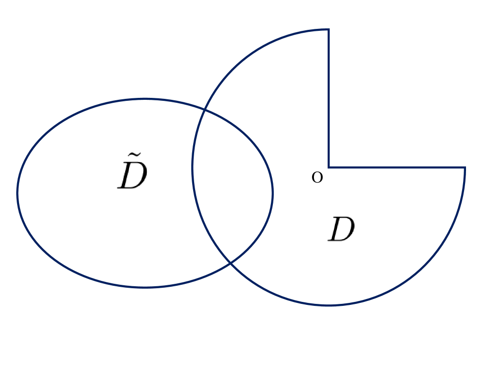
Figure 1: Penetrable scatterers $D$ and $\tilde{D}$ cannot produce identical outgoing waves (far-field patterns) due to the right corner $O$ lying on the boundary of the unbounded component of ${\mathbb{R}}^{2}\backslash\overline{D\cup\tilde{D}}$.

As we shall see from the proof of Theorem 1.1, a right corner scatters any incoming electric wave non-trivially in the TE case, as stated in the following corollary.

Corollary 1.3.

Let $\Omega=D\times{\mathbb{R}}$ be an infinitely long penetrable scatterer of cylindrical type and $u^{in}$ be any incoming wave such that

$$\Delta u^{in}+\kappa^{2}u^{in}=0,\quad{\rm div\,}u^{in}=0\qquad\mbox{in a neighbourhood of $D$}.$$

If $\partial D$ possesses a right corner, then the scattered field $u^{sc}$ corresponding to the transmission problem (1.1)-(1.4) cannot vanish identically in $D^{e}$.

It is easy to observe that, in the TE polarization case, the magnetic field is of the form $H(\textbf{x})=(0,0,v(x))$, where the scalar function $v:=1/(i\kappa)\nabla\times u$ is governed by the Helmholtz equation

$$\Delta v+\kappa^{2}q\;v=0\quad\mbox{in}\quad{\mathbb{R}}^{2},$$ (1.7)

together with the transmission conditions

$$v^{+}=v^{-},\quad\partial_{\nu}v^{+}=\lambda\;\partial_{\nu}v^{-}\quad\mbox{on}\quad\partial D.$$ (1.8)

Here $\lambda:=1/q_{0}\neq 1$ and $v=v^{in}+v^{sc}$ in ${\mathbb{R}}^{2}\backslash\overline{D}$, with

$$v^{in}(x)=1/(i\kappa)\nabla\times u^{in}(x)=-e^{i\kappa x\cdot d},\quad v^{sc}(x)=1/(i\kappa)\nabla\times u^{sc}(x).$$

One can derive from (1.5) that $v^{sc}$ fulfills the two-dimensional Sommerfeld radiation condition

$$\lim_{r\rightarrow\infty}\sqrt{r}\,\left(\partial_{r}v^{sc}-i\kappa v^{sc}\right)=0,\quad r=|x|.$$

In the current paper we do not consider the equivalent scalar transmission problem (1.7)-(1.8), because the subsequent analysis for the two-dimensional Maxwell equation (1.1)-(1.4) would provide us more insights into a possible approach for treating the full Maxwell system in three dimensions. The 3D case appears much more challenging than the planar case, and is still an open fundamental problem in inverse medium scattering problems. On the other hand, the transmission conditions in (1.4) keep the continuity of the Cauchy data $(\nabla\times u,\tau\cdot u)$ of the 2D Maxwell system across the interface $\partial D$. These conditions can be more easily handled by our approach than the transmission conditions (1.8) with $\lambda\neq 1$. The transmission problem (1.7)-(1.8) with $\lambda=1$ corresponds to the TM (transverse magnetic) polarization of our scattering problem, for which the electric and magnetic fields are of the form

$$E({\rm\textbf{x}})=(0,0,v(x)),\quad H({\rm\textbf{x}})=(u_{1}(x),u_{2}(x),0),\quad{\rm\textbf{x}}=(x,0)\in{\mathbb{R}}^{3}.$$

We refer to [1, 8, 5, 6, 20] for recent studies on inverse transmission problems of the scalar Helmholtz equation with $\lambda=1$ (i.e., the refractive index $q$ is continuous or has no jumps across the interface between the homogeneous and inhomogeneous media), not only in two dimensions but also in higher dimensions. It was shown that, under the assumption $\lambda=1$, the global and local uniqueness results as stated in Theorem 1.1 and Corollary 1.2 remain valid for curvilinear polygonal and polyhedral scatterers with variable potential functions (see [6]), and that one-dimensional interfaces with even a "weakly" singular point always scatter incoming waves non-trivially (see [16]). The arguments in these references do not apply to our current case of $\lambda\neq 1$, because the jumps of the normal derivatives would bring essential difficulties. To the best of our knowledge, no uniqueness results with a single incoming wave are available for $\lambda\neq 1$ and piecewise constant $q(x)$. It is worth noting that the case $q\equiv q_{0}$ in ${\mathbb{R}}^{2}$ (that is, the wave speed remains constant in the whole space) was verified by Ikehata in [10] for convex penetrable polygonal obstacles, as a byproduct of the enclosure method. In this paper we investigate the more practical case that $q$ is a piecewise constant function. Our results apply automatically to the Helmholtz system (1.7)-(1.8), since it is equivalent to the two dimensional Maxwell system (1.1)-(1.4). A comparison of the essential differences between our arguments and results with the ones in the recent paper [17] on electromagnetic corner scattering will be made in Remark 2.2 of Section 2.

Remark 1.4.

The unique solvability of the scattering problem (1.1), (1.4) and (1.5) follows from that of (1.7)-(1.8). In fact, applying the integral equation method or the variational approach one can prove that the scalar problem (1.7)-(1.8) admits a unique solution $v\in H^{1}_{loc}({\mathbb{R}}^{2})$ (see e.g., [4] and [3, Chapter 5]). This implies that the original scattering problem (1.1), (1.4) and (1.5) has a unique solution

$$u\in X:=\{u\in L^{2}_{loc}({\mathbb{R}}^{2})^{2},\quad\nabla\times u\in H^{1}_{loc}({\mathbb{R}}^{2})\}.$$

Since $q$ is piecewise constant, by elliptic interior regularity (see [7]) it is easy to see that $u$ is analytic in both $D$ and $D^{e}$.

Let us also mention that, if $\Omega\subset{\mathbb{R}}^{3}$ is a bounded perfectly conducting obstacle of polyhedral type, its geometrical shape $\partial\Omega$ can be uniquely determined by a single electric far-field pattern $E^{\infty}(\hat{{\rm x}})$ for all $\hat{{\rm x}}\in{\mathbb{S}}^{2}$; we refer to [18, 19] for the analysis based on the reflection principle for the full Maxwell system. For general penetrable and impenetrable scatterers, uniqueness in shape identification and medium recovery can be proved if the far-field patterns for all incident directions and polarization vectors with a fixed wavenumber are available; see [4, Chapter 7.1], [11], [13, 14, 21] and references therein.

The remaining part of this paper is organized as follows. In the subsequent Section 2, we prove Theorem 1.1 and Corollaries 1.2 and 1.3, all of which are essentially built upon the results in Lemma 2.1. The proof of Lemma 2.1 will be given in Section 3 via induction arguments.

2 Proofs of the main results

In this section we prove our main results stated in the previous section, namely, Theorem 1.1 and Corollaries 1.2-1.3. For this, we need a fundamental auxiliary result, whose proof is postponed to Section 3.

Lemma 2.1.

Let $B=\{x:|x|<1\}$, $\Gamma=\{(x_{1},0):x_{1}\geq 0\}\cup\{(0,x_{2}):x_{2}\geq 0\}$. Then for any two distinct constants $q_{1}$ and $q_{2}$ in ${\mathbb{C}}$, the solutions $u$ and $v$ to the vector-valued Helmholtz equations

$$\left\{\begin{array}[]{lll}\Delta u+q_{1}u=0&&\mbox{in}\quad B,\\ \Delta v+q_{2}v=0&&\mbox{in}\quad B,\\ {\rm div}\,u={\rm div}\,v=0&&\mbox{in}\quad B,\\ \tau\cdot u=\tau\cdot v&&\mbox{on}\quad B\cap\Gamma,\\ \nabla\times u=\nabla\times v&&\mbox{on}\quad B\cap\Gamma\end{array}\right.$$ (2.1)

vanish identically in the unit ball $B$.

Lemma 2.1 shows a local property of the two-dimensional Maxwell system around a domain with a right corner: the Cauchy data of such two Maxwell equations cannot coincide on an interface with a right corner, if the wavenumbers involved are not identical.

With the help of Lemma 2.1, we can now establish our main results in Section 1. We will provide a detailed proof of Theorem 1.1, but omit the proofs of Corollaries 1.2 and 1.3 as they can be verified basically in the same manner as it is done below for Theorem 1.1.

To prove Theorem 1.1, we assume that $D$ and $\tilde{D}$ are the cross-sections of two infinitely long rectangular penetrable scatterers whose scattered fields are denoted by $u^{sc}$ and $\tilde{u}^{sc}$, respectively. Analogously, we let $u^{\infty}$ and $\tilde{u}^{\infty}$ be the far-field patterns of $u^{sc}$ and $\tilde{u}^{sc}$. Supposing that $u^{\infty}(\hat{x})=\tilde{u}^{\infty}(\hat{x})$ for all $\hat{x}\in{\mathbb{S}}$, we need to show $D=\tilde{D}$. Assume on the contrary that $D\neq\tilde{D}$, then we derive a contradiction below.

We first apply Rellich’s lemma (see [4]) to obtain

$$u^{sc}=\tilde{u}^{sc}\quad\mbox{in}\quad D^{e}\cap\tilde{D}^{e}.$$

If $D\neq\tilde{D}$, one can always find a right corner $O$ and a small number $\epsilon>0$ such that either $O\in\partial D$ and $B_{\epsilon}(O)\subset\tilde{D}^{e}$, or $O\in\partial\tilde{D}$ and $B_{\epsilon}(O)\subset D^{e}$. Without loss of generality, we suppose that the former case holds; see Figure 2. Note that if $D\cap\tilde{D}=\emptyset$, one can easily derive a contradiction by extending the scattered field to the whole space and then applying Rellich’s lemma.

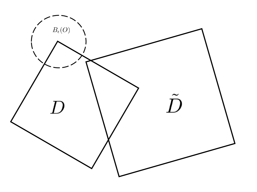
Figure 2: Two rectangular penetrable scatterers with the same far-field data.

Since the Maxwell system is invariant by both rotation and translation, we may suppose, without loss of generality, that the corner $O$ coincides with the origin and that the two sides of this right corner lie on the positive $ox_{1}$ and $ox_{2}$ axes, respectively. Then we have the following coupled system

$$\left\{\begin{array}[]{lll}\overrightarrow{\nabla}\times(\nabla\times u)-\kappa^{2}q_{0}u=0&&\mbox{in}\quad B_{\epsilon}(O)\cap D,\\ \overrightarrow{\nabla}\times(\nabla\times\tilde{u})-\kappa^{2}\tilde{u}=0&&\mbox{in}\quad B_{\epsilon}(O),\\ \tau\cdot u=\tau\cdot\tilde{u}&&\mbox{on}\quad B_{\epsilon}(O)\cap\partial D,\\ \nabla\times u=\nabla\times\tilde{u}&&\mbox{on}\quad B_{\epsilon}(O)\cap\partial D.\end{array}\right.$$

Since $\tilde{u}$ is analytic in $B_{\epsilon}(O)$ and the interface $B_{\epsilon}(O)\cap\partial D$ is piecewise analytic, the Cauchy pair $(\tau\cdot u,\nabla\times u)$ is piecewise analytic on the boundary $B_{\epsilon}(O)\cap\partial D$. Recalling the Cauchy-Kovalevskaya theorem, one may extend $u$ analytically from $\overline{D}\cap B_{\epsilon}(O)$ to a small neighborhood of the corner $O$ in the exterior domain $D^{e}\cap B_{\epsilon}(O)$. For notational convenience, we still denote by $B_{\epsilon}(O)$ the extended domain. Further, the extended function, which we still denote by $u$, satisfies the Maxwell equation

$$\overrightarrow{\nabla}\times(\nabla\times u)-\kappa^{2}q_{0}u=0\quad\mbox{in}\quad B_{\epsilon}(O).$$

Using the relation that $\overrightarrow{\nabla}\times(\nabla\times u)=-\Delta u+\nabla(\nabla\cdot u)$, we may apply Lemma 2.1 to $u$ and $\tilde{u}$ with $q_{1}=\kappa^{2}q_{0}$, $q_{2}=\kappa^{2}$ to deduce that both $u$ and $\tilde{u}$ vanish in $B_{\epsilon}(O)$, where we have used the assumption that $q_{0}\neq 1$. By the unique continuation of the Helmholtz equation, we have $u\equiv 0$ in ${\mathbb{R}}^{2}$. This is a contradiction to the fact that $|u^{in}|=1$ in ${\mathbb{R}}^{2}$ and $|u^{sc}|$ decays as $|x|$ tends to infinity. Hence, we have shown that $D=\tilde{D}$, and complete the proof of Theorem 1.1.

Remark 2.2.

We think that it is possible to prove Lemma 2.1 for the full Maxwell system in a cuboid domain in three dimensions. This was verified in [17] by using the CGO solutions for an admissible set of electric and magnetic fields which contain both electromagnetic planar waves and dipoles. Using this result, it was proved in [17] that the scattered fields do not vanish within the admissible set. But we emphasize that this result can not lead to any uniqueness result to the inverse scattering problem with a single incoming wave. In this work, we are able to demonstrate that any solution to the transmission problem of the two dimensional Maxwell system of the form in Lemma 2.1 must vanish. This excludes the inadmissible set considered in [17] for the TE case, hence help us establish the unique identifiability for the inverse medium scattering with a single incoming wave. Our studies show that the uniqueness issue is more difficult than the corner scattering problems that try to justify the non-vanishing of the scattered fields.

3 Proof of Lemma 2.1

We shall make full use of the expansion of the solutions to the Helmholtz equation in the Cartesian coordinate system to prove Lemma 2.1. We find the expansion in Cartesian coordinates particularly convenient for verifying Lemma 2.1 in domains with a right corner. The expansion in Cartesian coordinates was proved to be an effective approach for the scalar Helmholtz equation [5], but we encountered essential technical difficulties in our efforts to apply this approach to the current vector-valued Helmholtz equations.

Since $u$ and $v$ are the solutions to the Helmholtz equation with constant potentials, the functions $u$ and $v$ are both analytic in $B$. Hence $u$ and $v$ can be expanded in Taylor expansion:

$$u=\sum_{n\geq 0}\sum_{m\geq 0}U_{n,m}\,x_{1}^{n}x_{2}^{m}:=\sum_{n\geq 0}\sum_{m\geq 0}(u_{n,m}^{(1)},u_{n,m}^{(2)})\,x_{1}^{n}x_{2}^{m}\,,$$ (3.1)

$$v=\sum_{n\geq 0}\sum_{m\geq 0}V_{n,m}\,x_{1}^{n}x_{2}^{m}:=\sum_{n\geq 0}\sum_{m\geq 0}(v_{n,m}^{(1)},v_{n,m}^{(2)})\,x_{1}^{n}x_{2}^{m}$$ (3.2)

for $U_{n,m}=(u_{n,m}^{(1)},u_{n,m}^{(2)})\in{\mathbb{C}}^{2}$ and $V_{n,m}=(v_{n,m}^{(1)},v_{n,m}^{(2)})\in{\mathbb{C}}^{2}$. By plugging the expansions into the Helmholtz equations in (2.1), we easily derive the relations satisfied by $U_{n,m}$ and $V_{n,m}$:

$$\begin{split}&(n+1)(n+2)U_{n+2,m}+(m+1)(m+2)U_{n,m+2}+q_{1}U_{n,m}=0,\\ &(n+1)(n+2)V_{n+2,m}+(m+1)(m+2)V_{n,m+2}+q_{2}V_{n,m}=0.\end{split}$$ (3.3)

Let $A_{n,m}:=U_{n,m}-V_{n,m}=(a_{n,m}^{(1)},a_{n,m}^{(2)})$. Then it is easy to see the difference $w=u-v$ admits the Taylor expansion

$$w=\sum_{n\geq 0}\sum_{m\geq 0}A_{n,m}\,x_{1}^{n}x_{2}^{m}=\sum_{n\geq 0}\sum_{m\geq 0}(a_{n,m}^{(1)},a_{n,m}^{(2)})\,x_{1}^{n}x_{2}^{m}\quad\mbox{in}\quad B$$ (3.4)

and satisfies the equation

$$\Delta w+q_{1}w=(q_{2}-q_{1})v\quad\mbox{in}\quad B.$$ (3.5)

We first derive some important relations for the coefficients $a_{n,m}^{(j)}$ in (3.4).

Lemma 3.1.

For $j=1,2$ and all $n,m\geq 0$, the coefficients $a_{n,m}^{(j)}$ in (3.4) satisfy

$$\begin{split}&(m+4)(m+3)(m+2)(m+1)a^{(j)}_{n,m+4}+(n+4)(n+3)(n+2)(n+1)a^{(j)}_{n+4,m}\\ &+2(n+2)(n+1)(m+2)(m+1)a^{(j)}_{n+2,m+2}+(q_{1}+q_{2})(n+2)(n+1)a^{(j)}_{n+2,m}\\ &+(q_{1}+q_{2})(m+2)(m+1)a^{(j)}_{n,m+2}+q_{2}q_{1}a^{(j)}_{n,m}=0\,,\end{split}$$ (3.6)

$$(n+1)a^{(1)}_{n+1,m}=-(m+1)a^{(2)}_{n,m+1}\,,$$ (3.7)

$$a^{(1)}_{n,0}=0,\quad a^{(2)}_{0,m}=0\,,$$ (3.8)

$$(n+1)a^{(2)}_{n+1,0}=a^{(1)}_{n,1},\ a^{(2)}_{1,m}=(m+1)a^{(1)}_{0,m+1}\,.$$ (3.9)

Proof.

Using the expression (3.4) and the equation (3.5), we derive by direct computing that the coefficients $a^{(j)}_{n,m}$ fulfill the recursive relations

$$(n+1)(n+2)a^{(j)}_{n+2,m}+(m+1)(m+2)a^{(j)}_{n,m+2}+q_{1}a^{(j)}_{n,m}=(q_{2}-q_{1})v^{(j)}_{n,m}$$

for $j=1,2$, or equivalently, the coefficients $v^{(j)}_{n,m}$ satisfy that for all $n,m\geq 0$,

$$v^{(j)}_{n,m}=\frac{1}{q_{2}-q_{1}}\left[(n+1)(n+2)a^{(j)}_{n+2,m}+(m+1)(m+2)a^{(j)}_{n,m+2}+q_{1}a^{(j)}_{n,m}\right].$$ (3.10)

Then the desired results in (3.6) follow by inserting (3.10) in the second equation of (3.3). On the other hand, the relations (3.7) can follow directly from the divergence-free condition of $w=u-v$ (see (2.1)). Now using the transmission conditions that $\tau\cdot w=\nabla\times w=0\ \mbox{on}\ B\cap\Gamma$ (see (2.1)), we can obtain the desired relations (3.8)-(3.9). ∎

In the rest of this section we shall establish the desired results in Lemma 2.1 by proving $a^{(1)}_{n,m}=a^{(2)}_{n,m}=0$ for all $n,m\in{\mathbb{N}}^{+}$. Then it follows from (3.10) that $v_{n,m}^{(j)}=0$ for all $n,m\in{\mathbb{N}}^{+}$ and $j=1,2$, leading to $v\equiv 0$ by analyticity. Analogously, the vanishing of $u$ follows from the relation

$$u^{(j)}_{n,m}=\frac{1}{q_{2}-q_{1}}\left[(n+1)(n+2)a^{(j)}_{n+2,m}+(m+1)(m+2)a^{(j)}_{n,m+2}+q_{2}a^{(j)}_{n,m}\right].$$

Our proof is essentially based on an sophisticated induction argument on $M:=n+m=0,1,2,\cdots$, making full use of the relations (3.6)-(3.9).

It is easy to observe that there are a total of $2(M+1)$ coefficients $a^{(j)}_{n,m}$ ($j=1,2$) for each fixed $M=n+m$, while (3.7)-(3.9) give $M+2$ linear relations with $M-2$ unknown coefficients; see the diagram below where the line segment means a linear relation between the entries at two ends of the segment:

$$\begin{pmatrix}a_{M,0}^{(1)}\\ a_{M,0}^{(2)}\end{pmatrix}\diagdown\begin{pmatrix}a_{M-1,1}^{(1)}\\ a_{M-1,1}^{(2)}\end{pmatrix}\diagdown\begin{pmatrix}a_{M-2,2}^{(1)}\\ a_{M-2,2}^{(2)}\end{pmatrix}\diagdown\cdots\diagdown\begin{pmatrix}a_{2,M-2}^{(1)}\\ a_{2,M-2}^{(2)}\end{pmatrix}\diagdown\begin{pmatrix}a_{1,M-1}^{(1)}\\ a_{1,M-1}^{(2)}\end{pmatrix}\diagdown\begin{pmatrix}a_{0,M}^{(1)}\\ a_{0,M}^{(2)}\end{pmatrix},$$

$$\begin{pmatrix}a_{M,0}^{(1)}\\ a_{M,0}^{(2)}\end{pmatrix}\diagup\begin{pmatrix}a_{M-1,1}^{(1)}\\ a_{M-1,1}^{(2)}\end{pmatrix},\qquad\qquad\qquad\qquad\qquad\qquad\qquad\quad\begin{pmatrix}a_{1,M-1}^{(1)}\\ a_{1,M-1}^{(2)}\end{pmatrix}\diagup\begin{pmatrix}a_{0,M}^{(1)}\\ a_{0,M}^{(2)}\end{pmatrix}.$$

Our proof is divided in the following several lemmas.

Lemma 3.2.

The coefficients $a_{n,m}^{(j)}$ in (3.4) satisfy that $a^{(1)}_{n,m}=a^{(2)}_{n,m}=0$ for $n+m=0,1,2$.

Proof.

By setting $n,m=0,1$ in (3.8) we obtain

$$a^{(1)}_{0,0}=a^{(1)}_{1,0}=a^{(2)}_{0,0}=a^{(2)}_{1,0}=0.$$ (3.11)

This, together with (3.7) and (3.9), gives $a^{(1)}_{0,1}=a^{(2)}_{0,1}=0$. Then taking $n,m=2$ in (3.8), we see $a^{(1)}_{2,0}=a^{(2)}_{0,2}=0$. Further, by setting $(n,m)=(0,1),(1,0)$ in (3.7), respectively, we derive

$$a^{(1)}_{1,1}=-a_{0,2}^{(2)}=0,\quad a^{(2)}_{1,1}=-2a_{2,0}^{(1)}=0.$$

Finally, taking $(n,m)=(1,1)$ in (3.9) and using (3.11) we readily deduce

$$a^{(1)}_{0,2}=\frac{1}{2}a_{1,0}^{(2)}=0,\quad a^{(2)}_{2,0}=\frac{1}{2}a_{1,0}^{(1)}=0.$$

∎

Lemma 3.3.

All the coefficients $a_{n,m}^{(j)}$ in (3.4) with $n+m=3,5$ can be expressed by one parameter, respectively, namely

$$\begin{split}&a^{(1)}_{3,0}=0,\quad a^{(1)}_{2,1}=3\eta,\quad a^{(1)}_{1,2}=0,\quad\quad a^{(1)}_{0,3}=-\eta,\\ &a^{(2)}_{3,0}=\eta,\quad a^{(2)}_{2,1}=0,\quad\;a^{(2)}_{1,2}=-3\eta,\quad a^{(2)}_{0,3}=0\end{split}$$ (3.12)

and

$$\begin{split}&a^{(1)}_{5,0}=0,\;a^{(1)}_{4,1}=5\eta_{1},\;a^{(1)}_{3,2}=0,\qquad a^{(1)}_{2,3}=-10\eta_{1},\;a^{(1)}_{1,4}=0,\;\;a^{(1)}_{0,5}=\eta_{1}\\ &a^{(2)}_{5,0}=\eta_{1},\;a^{(2)}_{4,1}=0,\;\;a^{(2)}_{3,2}=-10\eta_{1},\;a^{(2)}_{2,3}=0,\quad\quad a^{(2)}_{1,4}=5\eta_{1},\;a^{(2)}_{0,5}=0\end{split}$$ (3.13)

for some $\eta,\eta_{1}\in\mathbb{R}$.

Proof.

We start with $n+m=3$. Setting $n,m=3$ in (3.8) and $(n,m)=(2,0),(1,1),(0,2)$ in (3.7), respectively, then $(n,m)=(2,1)$ in (3.9), we readily get

$$a^{(1)}_{3,0}=0,\quad a^{(2)}_{0,3}=0,\quad a^{(2)}_{2,1}=0,\quad a^{(1)}_{2,1}=-a^{(2)}_{1,2},\quad a^{(1)}_{1,2}=0,\quad 3a^{(2)}_{3,0}=a^{(1)}_{2,1},\quad 3a^{(1)}_{0,3}=a^{(2)}_{1,2}.$$

From these relations, we can easily see that all the coefficients $a^{(j)}_{n,m}$ with $n+m=3$ can be expressed by one parameter, say $\eta\in\mathbb{R}$, as in (3.12).

For the case $n+m=5$, we do the same as we did above for $n+m=3$ by using the relations (3.7), (3.8) and (3.9) to represent all the coefficients $a^{(j)}_{n,m}$ (with $n+m=5$) in terms of three parameters, say $\eta_{1},\eta_{2},\eta_{3}\in{\mathbb{R}}$,

$$\begin{split}&a^{(1)}_{5,0}=0,\;\;a^{(1)}_{4,1}=5\eta_{1},\;a^{(1)}_{3,2}=\eta_{3},\quad\;\;a^{(1)}_{2,3}=-10\eta_{2},\;a^{(1)}_{1,4}=0,\;\quad a^{(1)}_{0,5}=\eta_{2}\\ &a^{(2)}_{5,0}=\eta_{1},\;a^{(2)}_{4,1}=0,\;\;a^{(2)}_{3,2}=-10\eta_{1},\;a^{(2)}_{2,3}=-\eta_{3},\;\quad a^{(2)}_{1,4}=5\eta_{2},\;a^{(2)}_{0,5}=0.\end{split}$$ (3.14)

Next, we utilize (3.6) to derive a possible relation between three parameters $\eta_{1},\eta_{2},\eta_{3}$ in (3.14). In fact, by setting $n=0,m=1,j=1$ in (3.6) and using the relations in (3.12) and (3.14) for $a_{n,m}^{(1)}$, we can deduce that

$$4!\times 5\eta_{1}-2\times 2\times 3\times 2\times 10\eta_{2}+5!\times\eta_{2}+(q_{1}+q_{2})2\times 3\eta-(q_{1}+q_{2})3\times 2\eta=0\,,$$

which implies $\eta_{1}=\eta_{2}$ by noting the fact that the last two terms in the above equation cancel out. Analogously, one can get $\eta_{3}=0$ by setting $n=1,m=0,j=2$ in (3.6). Consequently, the fact that $\eta_{1}=\eta_{2},\eta_{3}=0$ enables us to reduce (3.14) to the desired one-parameter system (3.13). ∎

Lemma 3.4.

The coefficients $a_{n,m}^{(j)}$ in (3.4) satisfy that $a^{(1)}_{n,m}=a^{(2)}_{n,m}=0$ for $n+m=2k+1$, with all $k\geq 1$.

Proof.

With the results in Lemma 3.3 for $k=1,2$, namely $n+m=3,5$, we may expect that the coefficients $a_{n,m}^{(j)}$ with $M:=n+m=2k+1$ for any number $k\geq 3$ can also be expressed in some parameters. To verify this, we write all these coefficients in terms of $M-2=2k-1$ parameters in two groups: $c_{1},c_{2},\cdots,c_{\frac{M-1}{2}}$ and $b_{1},b_{2},\cdots,b_{\frac{M-3}{2}}$. More precisely, we may assume by using (3.7)-(3.9) that

$$\begin{split}&&\begin{pmatrix}a_{M,0}^{(1)}\\ a_{M,0}^{(2)}\end{pmatrix}=\begin{pmatrix}0\\ c_{1}\end{pmatrix},\quad\begin{pmatrix}a_{M-1,1}^{(1)}\\ a_{M-1,1}^{(2)}\end{pmatrix}=\begin{pmatrix}Mc_{1}\\ 0\end{pmatrix},\quad\begin{pmatrix}a_{M-2,2}^{(1)}\\ a_{M-2,2}^{(2)}\end{pmatrix}=\begin{pmatrix}b_{1}\\ -\frac{M(M-1)}{2}c_{1}\end{pmatrix},\hskip 28.45274pt\\ &&\begin{pmatrix}a_{M-3,3}^{(1)}\\ a_{M-3,3}^{(2)}\end{pmatrix}=\begin{pmatrix}c_{2}\\ -\frac{M-2}{3}b_{1}\end{pmatrix},\qquad\cdots,\qquad\begin{pmatrix}a_{3,M-3}^{(1)}\\ a_{3,M-3}^{(2)}\end{pmatrix}=\begin{pmatrix}b_{\frac{M-3}{2}}\\ -\frac{4}{M-3}c_{\frac{M-3}{2}}\end{pmatrix},\hskip 28.45274pt\\ &&\begin{pmatrix}a_{2,M-2}^{(1)}\\ a_{2,M-2}^{(2)}\end{pmatrix}=\begin{pmatrix}-\frac{M(M-1)}{2}c_{\frac{M-1}{2}}\\ -\frac{3}{M-2}b_{\frac{M-3}{2}}\end{pmatrix},\quad\begin{pmatrix}a_{1,M-1}^{(1)}\\ a_{1,M-1}^{(2)}\end{pmatrix}=\begin{pmatrix}0\\ Mc_{\frac{M-1}{2}}\end{pmatrix},\quad\begin{pmatrix}a_{0,M}^{(1)}\\ a_{0,M}^{(2)}\end{pmatrix}=\begin{pmatrix}c_{\frac{M-1}{2}}\\ 0\end{pmatrix}.\end{split}$$ (3.15)

Then the desired results in Lemma 3.4 are a consequence of the following two steps, first to show all $c_{j}$ in (3.15) vanish (Step 1), then to prove the same for all $b_{j}$ above (Step 2).

Step 1: Prove that $c_{j}=0$ for all $j=1,\cdots,(M-1)/2$.

For the purpose of induction, we rewrite the relations in (3.13) (that is, $k=2$ or $M=5$) involving the non-vanishing parameters in a more general form as follows:

$$\begin{split}&a^{(1)}_{M-1,1}=M\eta_{M},~{}a^{(1)}_{M-3,3}=-\frac{M!}{(M-3)!3!}\eta_{M},\;\cdots,~{}a^{(1)}_{4,M-4}=(-1)^{\frac{M-5}{2}}\frac{M!}{(M-4)!4!}\eta_{M}{\color[rgb]{1.000,0.000,0.000},}\\ &a^{(1)}_{2,M-2}=(-1)^{\frac{M-3}{2}}\frac{M(M-1)}{2}\eta_{M},~{}a^{(2)}_{M-2,2}=-\frac{M(M-1)}{2}\eta_{M},~{}a^{(1)}_{0,M}=(-1)^{\frac{M-1}{2}}\eta_{M},\\ &a^{(2)}_{M,0}=\eta_{M},~{}a^{(2)}_{M-4,4}=\frac{M!}{(M-4)!4!}\eta_{M},~{}a^{(2)}_{M-6,6}=-\frac{M!}{(M-6)!6!}\eta_{M},\cdots\,\\ &a^{(2)}_{3,M-3}=(-1)^{\frac{M-3}{2}}\frac{M!}{(M-3)!3!}\eta_{M},~{}a^{(2)}_{1,M-1}=(-1)^{\frac{M-1}{2}}M\eta_{M}.\end{split}$$ (3.16)

Note that the constant $\eta_{1}$ in (3.13) has been replaced by $\eta_{M}$ and that the coefficients before $\eta_{M}$ in the above relations are derived from (3.7)-(3.9). This confirms that for $M=5$ (or $k=2$), the coefficients in (3.15) related to $c_{j}$ $(j=1,2,\cdots,c_{\frac{M-1}{2}})$ depend only on $\eta_{M}$. For any fixed $k\geq 3$, i.e., $M\geq 7$, we now verify all the relations in (3.16) under the induction hypothesis that

$$\begin{split}&a^{(1)}_{M^{{}^{\prime}}-1,1}=M^{{}^{\prime}}\eta_{M^{{}^{\prime}}},~{}a^{(1)}_{M^{{}^{\prime}}-3,3}=-\frac{M^{{}^{\prime}}!}{(M^{{}^{\prime}}-3)!3!}\eta_{M^{{}^{\prime}}},\cdots\,,~{}a^{(1)}_{4,M^{{}^{\prime}}-4}=(-1)^{\frac{M^{{}^{\prime}}-5}{2}}\frac{M^{{}^{\prime}}!}{(M^{{}^{\prime}}-4)!4!}\eta_{M^{{}^{\prime}}}\\ &a^{(1)}_{2,M^{{}^{\prime}}-2}=(-1)^{\frac{M^{{}^{\prime}}-3}{2}}\frac{M^{{}^{\prime}}(M^{{}^{\prime}}-1)}{2}\eta_{M^{{}^{\prime}}},~{}a^{(1)}_{0,M^{{}^{\prime}}}=(-1)^{\frac{M^{{}^{\prime}}-1}{2}}\eta_{M^{{}^{\prime}}}\\ &a^{(2)}_{M^{{}^{\prime}},0}=\eta_{M^{{}^{\prime}}},~{}a^{(2)}_{M^{{}^{\prime}}-2,2}=-\frac{M^{{}^{\prime}}(M^{{}^{\prime}}-1)}{2}\eta_{M^{{}^{\prime}}},~{}a^{(2)}_{M^{{}^{\prime}}-4,4}=\frac{M^{{}^{\prime}}!}{(M^{{}^{\prime}}-4)!4!}\eta_{M^{{}^{\prime}}},\cdots\,\\ &a^{(2)}_{3,M^{{}^{\prime}}-3}=(-1)^{\frac{M^{{}^{\prime}}-3}{2}}\frac{M^{{}^{\prime}}!}{(M^{{}^{\prime}}-3)!3!}\eta_{M^{{}^{\prime}}},~{}a^{(2)}_{1,M^{{}^{\prime}}-1}=(-1)^{\frac{M^{{}^{\prime}}-1}{2}}M^{{}^{\prime}}\eta_{M^{{}^{\prime}}},\end{split}$$ (3.17)

for all $M^{\prime}=2k^{\prime}+1$, $k^{\prime}=0,1,\cdots,k-1$. This implies that all the coefficients in (3.15) related to $c_{j}$ depend actually on one parameter. For this purpose, it suffices to verify that the coefficients $a_{n,m}^{(j)}$ in (3.16) satisfying $n+m=M$ can be represented by the unique parameter $\eta_{M}$. To do so, we take $n=M-4,m=0,j=2$ and $n=M-5,m=1,j=1$ in (3.6), respectively, and utilize the induction hypothesis above to come readily to the relations

$$\Big{\{}\frac{M!}{(M-4)!}a^{(2)}_{M,0}-2\frac{M!}{(M-4)!}\Big{\}}c_{1}-6(M-3)c_{2}+q_{1}q_{2}\eta_{M-4}=0,$$ (3.18)

$$\frac{M!}{(M-5)!}c_{1}+12(M-3)(M-4)c_{2}+120c_{3}+(M-4)q_{1}q_{2}\eta_{M-4}=0.$$ (3.19)

Analogously, setting $j=1$, $n=M-2k-5$ and $m=2k+1$ for all $1<k\leq{(M-5)}/{2}$ in (3.6), we obtain in combination of (3.18) and (3.19) the following linear system

$$A_{M}\,X_{M}=B_{M},$$ (3.20)

where $A_{M}$, $B_{M}$ and $X_{M}$ are given by

$$A_{M}=\begin{pmatrix}\begin{smallmatrix}-\frac{M!}{(M-4)!}&-(M-3)3\times 2&0&\dots&0&0\\ \frac{M!}{(M-5)!}&2(M-3)(M-4)3\times 2&5\times 4\times 3\times 2&0&\dots&0\\ 0&(M-3)(M-4)(M-5)(M-6)&2(M-5)(M-6)5\times 4&7\times 6\times 5\times 4&0&0\\ 0&0&\ddots&\ddots&\ddots&\vdots\\ 0&\dots&0&6\times 5\times 4\times 3&2(M-4)(M-5)3\times 4&-\frac{\frac{(M)!}{(M-6)!}}{2}\\ 0&\dots&0&0&4\times 3\times 2&-\frac{M!}{(M-4)!}\end{smallmatrix}\end{pmatrix},$$

$$B_{M}=\begin{pmatrix}\begin{smallmatrix}&\eta_{M-4}\\ &(M-4)\eta_{M-4}\\ &-\frac{(M-4)!}{(M-7)!3!}\eta_{M-4}\\ &\vdots\\ &(-1)^{\frac{M-7}{2}}\frac{(M-4)(M-5)}{2}\eta_{M-4}\\ &(-1)^{\frac{M-5}{2}}\eta_{M-4}\end{smallmatrix}\end{pmatrix},\quad X_{M}=\begin{pmatrix}\begin{smallmatrix}&c_{1}\\ &c_{2}\\ &\vdots\\ &c_{\frac{M-1}{2}}\end{smallmatrix}\end{pmatrix}\,.$$

We next demonstrate $\eta_{M-4}=0$ by diagonalizing the matrix $A_{M}$. To this aim, we form the augmented matrix $\widetilde{A}=[A_{M},B_{M}]$:

$$\begin{pmatrix}\begin{smallmatrix}-\frac{M!}{(M-4)!}&-6(M-3)&0&\dots&0&0&\eta_{M-4}\\ \frac{M!}{(M-5)!}&12(M-3)(M-4)&5\times 4\times 3\times 2&0&\dots&0&(M-4)\eta_{M-4}\\ 0&\frac{(M-3)!}{(M-7)!}&2(M-5)(M-6)5\times 4&7\times 6\times 5\times 4&0&0&-\frac{(M-4)!}{(M-7)!3!}\eta_{M-4}\\ 0&0&\ddots&\ddots&\ddots&\vdots&\vdots\\ 0&\dots&0&6\times 5\times 4\times 3&2(M-4)(M-5)3\times 4&-\frac{(M)!}{2(M-6)!}&(-1)^{\frac{M-7}{2}}\frac{(M-4)(M-5)}{2}\eta_{M-4}\\ 0&\dots&0&0&4\times 3\times 2&-\frac{M!}{(M-4)!}&(-1)^{\frac{M-5}{2}}\eta_{M-4}.\end{smallmatrix}\end{pmatrix}.$$

Below we shall often write as $r_{j}$ the $j$-th row of the matrix $\widetilde{A}$ or the transformed variant of $\widetilde{A}$ by an elementary transformation. By applying $r_{1}\times(M-4)+r_{2}$ to $\widetilde{A}$, we have the matrix $\widetilde{A}_{1}$:

$$\begin{pmatrix}\begin{smallmatrix}-\frac{M!}{(M-4)!}&-6(M-3)&0&\dots&0&0&\eta_{M-4}\\ 0&6(M-3)(M-4)&5\times 4\times 3\times 2&0&\dots&0&2(M-4)\eta_{M-4}\\ 0&\frac{(M-3)!}{(M-7)!}&2(M-5)(M-6)5\times 4&7\times 6\times 5\times 4&0&0&-\frac{(M-4)!}{(M-7)!3!}\eta_{M-4}\\ 0&0&\ddots&\ddots&\ddots&\vdots&\vdots\\ 0&\dots&0&6\times 5\times 4\times 3&2(M-4)(M-5)3\times 4&-\frac{(M)!}{2(M-6)!}&(-1)^{\frac{M-7}{2}}\frac{(M-4)(M-5)}{2}\eta_{M-4}\\ 0&\dots&0&0&4\times 3\times 2&-\frac{M!}{(M-4)!}&(-1)^{\frac{M-5}{2}}\eta_{M-4}\end{smallmatrix}\end{pmatrix}\,,$$

to which we apply the transformation $-\frac{r_{2}\times(M-5)(M-6)}{6}+r_{3}$ to get the matrix $\widetilde{A}_{2}$:

$$\begin{pmatrix}\begin{smallmatrix}-\frac{M!}{(M-4)!}&-6(M-3)&0&\dots&0&0&\eta_{M-4}\\ 0&6(M-3)(M-4)&5\times 4\times 3\times 2&0&\dots&0&2(M-4)\eta_{M-4}\\ 0&0&20(M-5)(M-6)&7\times 6\times 5\times 4&0&0&-3\frac{(M-4)!}{(M-7)!3!}\eta_{M-4}\\ 0&0&\ddots&\ddots&\ddots&\vdots&\vdots\\ 0&\dots&0&6\times 5\times 4\times 3&2(M-4)(M-5)3\times 4&-\frac{(M)!}{2(M-6)!}&(-1)^{\frac{M-7}{2}}\frac{(M-4)(M-5)}{2}\eta_{M-4}\\ 0&\dots&0&0&4\times 3\times 2&-\frac{M!}{(M-4)!}&(-1)^{\frac{M-5}{2}}\eta_{M-4}\end{smallmatrix}\end{pmatrix}.$$

Repeating the above process, we come to the matrix $\widetilde{A}_{\frac{M-3}{2}-1}$:

$$\begin{pmatrix}\begin{smallmatrix}-\frac{M!}{(M-4)!}&-6(M-3)&0&\dots&0&0&\eta_{M-4}\\ 0&6(M-3)(M-4)&5\times 4\times 3\times 2&0&\dots&0&2(M-4)\eta_{M-4}\\ 0&0&20(M-5)(M-6)&7\times 6\times 5\times 4&0&0&-3\frac{(M-4)!}{(M-7)!3!}\eta_{M-4}\\ 0&0&\ddots&\ddots&\ddots&\vdots&\vdots\\ 0&\dots&0&0&(M-4)(M-5)3\times 4&-\frac{(M)!}{2(M-6)!}&(\frac{M-3}{2})(-1)^{\frac{M-7}{2}}\frac{(M-4)(M-5)}{2}\eta_{M-4}\\ 0&\dots&0&0&4\times 3\times 2&-\frac{M!}{(M-4)!}&(-1)^{\frac{M-5}{2}}\eta_{M-4}\end{smallmatrix}\end{pmatrix}.$$

Now, taking the action $-r_{\frac{M-3}{2}}\times\frac{2}{(M-4)(M-5)}+r_{\frac{M-1}{2}}$, we may transform $\widetilde{A}_{\frac{M-3}{2}-1}$ into a new matrix whose last row is given by

$$\begin{pmatrix}0&\cdots&0&0&0&0&(-1)^{\frac{M-5}{2}}(\eta_{M-4}+(\frac{M-3}{2})\eta_{M-4})\end{pmatrix}\,.$$

This, along with the linear system (3.20), leads to the relation

$$(-1)^{\frac{M-5}{2}}(\eta_{M-4}+(\frac{M-3}{2})\eta_{M-4})=0,$$

from which we see that

$$\eta_{M-4}=0.$$ (3.21)

Now, the nonhomogeneous system (3.20) reduces to the homogeneous one $A_{M}\,X_{M}=0$ because of the result (3.21). We can easily trace from the previous linear transformations we have applied to $A_{M}$ to know that

$$\mbox{rank}(A_{M})=\frac{M-1}{2}-1.$$ (3.22)

This means that the non-trivial solutions to $A_{M}X_{M}=0$ forms a one-dimensional space. Then we can directly derive from (3.20) by taking $c_{1}=\eta_{M}$ as a single parameter that

$$\begin{pmatrix}c_{1}\\ c_{2}\\ \vdots\\ c_{\frac{M-3}{2}}\\ c_{\frac{M-1}{2}}\\ \end{pmatrix}=\begin{pmatrix}\eta_{M}\\ -\frac{M!}{(M-3)!3!}\eta_{M}\\ \vdots\\ (-1)^{\frac{M-5}{2}}\frac{M!}{(M-4)!4!}\eta_{M}\\ (-1)^{\frac{M-1}{2}}\eta_{M}\,,\end{pmatrix}$$ (3.23)

hence prove the relations in (3.16) for all $M\geq 7$. By the arbitrariness of $M=2k+1$ for $k\geq 3$ and induction argument, we can conclude that $\eta_{M}=0$ for all odd integers $M\in{\mathbb{N}}^{+}$, and in particular, the vanishing of $c_{j}$, $j=1,2,\cdots,c_{{(M-1)}/{2}}$.

Step 2: Prove that $b_{j}=0$ for all $j=1,2,\cdots,{(M-3)}/{2}$, and all $M=2k+1$ with $k\geq 3$. This yields the vanishing of the coefficients $a_{n,m}^{(j)}$ that depend on $b_{1},b_{2},\cdots,b_{{(M-3)}/{2}}$ in (3.15).

Again, we shall use the induction argument to prove that

$$\begin{split}&a^{(1)}_{M,0}=a^{(1)}_{M-2,2}=\cdots\,=a^{(1)}_{3,M-3}=a^{(1)}_{1,M-1}=0,\\ &a^{(2)}_{M-1,1}=0=a^{(2)}_{M-3,3}=\cdots\,=a^{(2)}_{2,M-2}=a^{(2)}_{0,M}=0,\end{split}$$ (3.24)

for all $M=2k+1$, $k\geq 3$. Note that the case of $k=2$ (or $M=5$) was verified in (3.13). We make the induction hypothesis that

$$\begin{split}&a^{(1)}_{M^{{}^{\prime}},0}=a^{(1)}_{M^{{}^{\prime}}-2,2}=\cdots\,=a^{(1)}_{3,M^{{}^{\prime}}-3}=a^{(1)}_{1,M^{{}^{\prime}}-1}=0\\ &a^{(2)}_{M^{{}^{\prime}}-1,1}=0=a^{(2)}_{M^{{}^{\prime}}-3,3}=\cdots\,=a^{(2)}_{2,M^{{}^{\prime}}-2}=a^{(2)}_{0,M^{{}^{\prime}}}=0,\end{split}$$

for all $M^{\prime}=2k^{\prime}+1$, $0\leq k^{\prime}<k$. Then by setting $j=1$, $n=M-4,m=0$ and $n=M-6,m=2$ in (3.6), respectively, and using the induction hypothesis, we obtain that

$$4\times(M-2)(M-3)b_{1}+4!b_{2}=0\,,$$ (3.25)

$$\frac{(M-2)!}{(M-6)!}b_{1}+2(M-4)(M-5)4\times 3b_{2}+6\times 5\times 4\times 3b_{3}=0.$$ (3.26)

We can continue this process, by taking $j=1$, $n=M-2k-4$ and $m=2k$ for any $2\leq k\leq\frac{M-5}{2}$ in (3.6), then using (3.25) and (3.26), to derive the homogeneous linear algebraic system

$$\tilde{G}_{M}Y_{M}=0,$$

where

$$\tilde{G}_{M}=\begin{pmatrix}\begin{smallmatrix}4\times(M-2)(M-3)&4!&\dots&0&0\\ (M-2)(M-3)(M-4)(M-5)&2(M-4)(M-5)4\times 3&6\times 5\times 4\times 3&\dots&0\\ 0&(M-4)(M-5)(M-6)(M-7)&2(M-6)(M-7)6\times 5&8\times 7\times 6\times 5&0\\ 0&\ddots&\ddots&\ddots&\vdots\\ \dots&0&7\times 6\times 5\times 4&2(M-5)(M-6)5\times 4&\frac{(M-3)!}{(M-7)!}\\ \dots&0&0&5\times 4\times 3\times 2&2(M-3)(M-4)6\end{smallmatrix}\end{pmatrix}$$

and

$$Y_{M}=\begin{pmatrix}b_{1},&b_{2},&\cdots\,&b_{\frac{M-3}{2}}&\end{pmatrix}^{\prime}.$$

It is easy to find through diagonalization that $\mbox{Det}(G_{M})\neq 0$, hence leading to the vanishing of $b_{j}$, $j=1,2,\cdots,{(M-3)}/{2}$. ∎

Lemma 3.5.

The coefficients $a_{n,m}^{(j)}$ in (3.4) satisfy that $a^{(1)}_{n,m}=a^{(2)}_{n,m}=0$ for $n+m=2k$, with all $k\geq 2$.

Proof.

The argument is carried out in a similar manner to the one for Lemma 3.4. We first show that $a^{(1)}_{n,m}=a^{(2)}_{n,m}=0$ for $k=2$, or $n+m=4$. To this aim, we set $n=m=4$ in (3.8) and $n=m=3$ in (3.9), respectively, to sfind that

$$a^{(1)}_{4,0}=a^{(2)}_{0,4}=0\quad\mbox{and}\quad 4a^{(2)}_{4,0}=a^{(1)}_{3,1},\quad 4a^{(1)}_{0,4}=a^{(2)}_{1,3}.$$

Then setting $n=n_{j},m=m_{j},n_{j}+m_{j}=3$ for $j=3,2,1,0$ in (3.7), respectively, we easily derive

$$a^{(2)}_{3,1}=0,\quad\frac{3}{2}a^{(1)}_{3,1}=-a^{(2)}_{2,2},\quad\frac{2}{3}a^{(1)}_{2,2}=-a^{(2)}_{1,3},\quad a^{(1)}_{1,3}=0.$$

Therefore, we are able to express all the coefficients $a_{n,m}^{(j)}$ with $n+m=4$ in two parameters $\eta_{1},\eta_{2}\in\mathbb{R}$ as follows:

$$\begin{split}&a^{(1)}_{4,0}=0,~{}a^{(1)}_{3,1}=4\eta_{1},a^{(1)}_{2,2}=-6\eta_{2},~{}a^{(1)}_{1,3}=0,~{}a^{(1)}_{0,4}=\eta_{2},\\ &a^{(2)}_{4,0}=\eta_{1},~{}a^{(2)}_{3,1}=0,~{}a^{(2)}_{2,2}=-6\eta_{1},~{}a^{(2)}_{1,3}=4\eta_{2},~{}a^{(2)}_{0,4}=0.\\ \end{split}$$ (3.27)

Furthermore, by taking $n=0,m=0$ in (3.6), we obtain

$$4\,!\,a_{0,4}^{(j)}+4\,!\,a_{4,0}^{(j)}+8a_{2,2}^{(j)}=0,\quad j=1,2,$$

which, along with (3.27), concludes that $\eta_{1}=\eta_{2}=0$. Therefore, we have shown that $a^{(j)}_{n,m}=0$ for all $n+m=4$ and $j=1,2$.

For any fixed $k\geq 3$, we make the induction hypothesis that

$$a_{n,m}^{(j)}=0\quad\mbox{for all}\quad M=n+m=2k^{{}^{\prime}},\;~{}0\leq k^{{}^{\prime}}<k.$$

Then we argue analogously to what we did for Lemma 3.4 to derive from (3.7)-(3.9) that

$$\begin{split}&a^{(1)}_{M-1,1}=Mc_{1},~{}a^{(1)}_{M-3,3}=c_{2},\;~{}\cdots\,,~{}a^{(1)}_{3,M-3}=c_{\frac{M}{2}-1},~{}a^{(1)}_{1,M-1}=0,\\ &a^{(2)}_{M,0}=c_{1},~{}a^{(2)}_{M-2,2}=-\frac{M(M-1)}{2}c_{1},\;\cdots\,,~{}a^{(2)}_{2,M-2}=-c_{\frac{M}{2}-1},~{}a^{(2)}_{0,M}=0,\\ \end{split}$$ (3.28)

and

$$\begin{split}&a^{(1)}_{M,0}=0,~{}a^{(1)}_{M-2,2}=b_{1},\;\cdots,\,~{}a^{(1)}_{2,M-2}=-\frac{M(M-1)}{2}b_{\frac{M}{2}-1},~{}a^{(1)}_{0,M}=b_{\frac{M}{2}-1},\\ &a^{(2)}_{M-1,1}=0,\quad a^{(2)}_{M-3,3}=\cdots\,=a^{(2)}_{1,M-1}=Mb_{\frac{M}{2}-1},\\ \end{split}$$ (3.29)

where $c_{1}$, $c_{2}$,$\cdots$, $c_{{M}/{2}-1}$ and $b_{1}$, $b_{2}$, $\cdots$, $b_{{M}/{2}-1}$ are all constants in ${\mathbb{C}}$.

Next, we show that all these constants are identically zero. To prove that all the constants $c_{j}$ for $j=1,2,\cdots,M/2-1$ are zero, we set $n=M-4,m=0,j=2$ and $n=M-5,m=1,j=1$ in (3.6), respectively, and use the induction hypothesis (3.28) to deduce that

$$[\frac{M!}{(M-4)!}a^{(2)}_{M,0}-2\frac{M!}{(M-4)!}]c_{1}-(M-3)3\times 2c_{2}=0\,,$$ (3.30)

$$\frac{M!}{(M-5)!}c_{1}+2(M-3)(M-4)3\times 2c_{2}+5\times 4\times 3\times 2c_{3}=0.$$ (3.31)

We can repeat this process by taking $j=1$ and $n=M-2k-5$,$m=2k+1$ for all $0<k\leq\frac{M-6}{2}$ in (3.6) to arrive at the linear system

$$A\,X=0,$$

where

$$A:=\begin{pmatrix}\begin{smallmatrix}-\frac{M!}{(M-4)!}&-(M-3)3\times 2&0&\dots&0&0\\ \frac{M!}{(M-5)!}&2(M-3)(M-4)3\times 2&5\times 4\times 3\times 2&0&\dots&0\\ 0&(M-3)(M-4)(M-5)(M-6)&2(M-5)(M-6)5\times 4&7\times 6\times 5\times 4&0&0\\ 0&0&\ddots&\ddots&\ddots&\vdots\\ 0&\dots&0&7\times 6\times 5\times 4&2(M-5)(M-6)5\times 4&\frac{(M-3)!}{(M-7)!}\\ 0&\dots&0&0&5\times 4\times 3\times 2&2(M-3)(M-4)3\times 2&\end{smallmatrix}\end{pmatrix},$$

and

$$X=\begin{pmatrix}c_{1},&c_{2},&\cdots\,&c_{\frac{M}{2}-1}&\end{pmatrix}^{{}^{\prime}}.$$

Again, by a diagonlization process we can directly verify that $\mbox{Det}(A)\neq 0$, implying that

$$c_{1}=c_{2}=\cdots\,=c_{\frac{M}{2}-1}=0.$$

It remains to show that all constants $b_{j}$ for $j=1,2,\cdots,M/2-1$ also vanish. For this, we set $n=0,m=M-4,j=1$ and $n=2,m=M-6,j=1$ in (3.6) respectively to see that

$$[\frac{M!}{(M-4)!}-2\frac{M!}{(M-4)!}]b_{\frac{M}{2}-1}+4\times 3\times b_{\frac{M}{2}-2}=0\,,$$ (3.32)

$$-\frac{M!}{2(M-6)!}b_{\frac{M}{2}-1}+2(M-4)(M-5)4\times 3b_{\frac{M}{2}-2}+6\times 5\times 4\times 3b_{{\frac{M}{2}}-3}=0.$$ (3.33)

Then we may continue this process by taking $j=1$ and $n=2k$,$m=M-2k-4$ for all $2\leq k\leq\frac{M-4}{2}$ in (3.6), to come up with the linear system

$$\tilde{A}\;Y=0,$$

where

$$\tilde{A}:=\begin{pmatrix}\begin{smallmatrix}-\frac{M!}{(M-4)!}&4\times 3\times 2&0&\dots&0&0\\ -\frac{\frac{M!}{(M-6)!}}{2}&2(M-4)(M-5)4\times 3&6\times 5\times 4\times 3&0&\dots&0\\ 0&(M-4)(M-5)(M-6)(M-7)&2(M-6)(M-7)6\times 5&8\times 7\times 6\times 5&0&0\\ 0&0&\ddots&\ddots&\ddots&\vdots\\ 0&\dots&0&6\times 4\times 3\times 2&2(M-4)(M-5)4\times 3&\frac{(M-2)!}{(M-6)!}\\ 0&\dots&0&0&4\times 3\times 2&4(M-2)(M-3)&\end{smallmatrix}\end{pmatrix},$$

and

$$Y=\begin{pmatrix}b_{\frac{M}{2}-1},&b_{\frac{M}{2}-2},&\cdots\,&b_{1}\end{pmatrix}^{{}^{\prime}}.$$

As we did earlier, we can verify that $\mbox{Det}(\tilde{A})\neq 0$, therefore derive the desired results that

$$b_{1}=b_{2}=\cdots=b_{\frac{M}{2}-1}=0.$$

∎

Now the result of Lemma 2.1 follows directly from Lemmas 3.2-3.5.

Remark 3.6.

We believe that it might be possible to prove Theorem 1.1 in a general planar corner domain whose angle lies in $(0,2\pi)\backslash\{\pi\}$. However, as one could expect, much more complicated technicalities will be involved in the proof of the analogue of Lemma 2.1 by our approach. The inverse transmission problem for the scalar Helmholtz equation (1.7)-(1.8) with such general angles also deserves further investigation.

4 Acknowledgments

The work of G. Hu is supported by the NSFC grant (No. 11671028) and NSAF grant (No. U1530401). The work of L. Li is partially supported by the National Science Foundation of China (61421062, 61520106004) and Microsoft Research of Asia. The work of J. Zou was supported by the Hong Kong RGC General Research Fund (project 14322516) and National Natural Science Foundation of China/Hong Kong Research Grants Council Joint Research Scheme 2016/17 (project N_CUHK437/16).

References

- [1] E. Blåsten, L. Päivärinta and J. Sylvester, Corners always scatter, Commun. Math. Phys., 331 (2014): 725–753.
- [2] J. Bramble and J. Pasciak, Analysis of a cartesian PML approximation to the three dimensional electromagnetic wave scattering problem, Int. J. Numer. Anal. Model. 9 (2012): 543-561.
- [3] F. Cakoni and D. Colton, A Qualitative Approach to Inverse Scattering Theory, Springer, Newyork, 2014.
- [4] D. Colton and R. Kress, Inverse Acoustic and Electromagnetic Scattering Theory, third edition, Springer, New York, 2013.
- [5] J. Elschner and G. Hu, Corners and edges always scatter, Inverse Problems, 31 (2015): 015003.
- [6] J. Elschner and G. Hu, Acoustic scattering from corners, edges and circular cones, Archive for Rational Mechanics and Analysis, 228 (2018): 653-690.
- [7] D. Gilbarg and N. Trudinger, Elliptic Partial Differential Equations of Second Order, Springer-Verlag, Heidelberg, 1977.
- [8] G. Hu, M. Salo, E. V. Vesalainen, Shape identification in inverse medium scattering problems with a single far-field pattern, SIAM J. Math. Anal., 48 (2016): 152–165.
- [9] Q. Hu, C. Liu, S. Shu and J. Zou, An effective preconditioner for a PML system for electromagnetic scattering problem. ESAIM Math. Model. Numer. Anal. 49 (2015): 839-854.
- [10] M. Ikehata, An inverse transmission scattering problem and the enclosure method, Computing 75 (2005): 133–156.
- [11] P. Hähner, A uniqueness theorem for a transmission problem in inverse electromagnetic scattering, Inverse Problems 9 (1993): 667-678.
- [12] A. Kirsch and R. Kress, Uniqueness in inverse obstacle scattering, Inverse Problems, 9 (1993): 285–299.
- [13] R. Kress, Uniquness in inverse obstacle scattering from electromagnetic waves, Proceedings of the URSI General Assembly 2002, Maastricht, availabe at: http://num.math.uni-goettingen.de/kress/ursi.pdf
- [14] R. Kress, Uniqueness in inverse obstacle scattering, New analytic and geometric methods in inverse problems, 323-336, Springer, Berlin, 2004.
- [15] S. Kusiak and J. Sylvester, The scattering support, Communications on Pure and Applied Mathematics, 56 (2003): 1525–1548.
- [16] L. Li, G. Hu and J. Yang, Interface with weakly singular points always scatter, Inverse Problems 34 (2018): 075003.
- [17] H. Liu and J. Xiao, Electromagnetic scattering from a penetrable corner, SIAM J. Math. Anal., 49 (2017): 5207-4241.
- [18] H. Liu, M. Yamamoto and J. Zou, Reflection principle for the Maxwell equations and its application to inverse electromagnetic scattering, Inverse Problems 23 (2007): 2357-2366.
- [19] H. Liu, M. Yamamoto and J. Zou, New reflection principles for Maxwell’s equations and their applications, Numer. Math. Theory Methods Appl. 2 (2009): 1-17.
- [20] L. Päivärinta, M. Salo and E. V. Vesalainen, Strictly convex corners scatter, Rev. Mat. Iberoam., 33 (2017): 1369-1396.
- [21] Z. Sun and G. Uhlmann, An inverse boundary value problem for Maxwell’s equations, Arch. Rat. Mech. Anal., 119 (1992): 71-93.