Perturbation initial conditions for a couple of dark energy scalar field potentials

Abstract

We present perturbation initial conditions for two types of scalar field potential often used in the dark energy study: one inverse power-law and the other exponential. The solutions are presented in the presence of the $w=$ constant fluid ($w=1/3$ for radiation fluid), a minimally coupled scalar field and a sub-dominating zero-pressure fluid (cold dark matter and baryon dust). We consider two gauge conditions, the $w$-fluid comoving gauge and the cold-dark-matter comoving gauge; solutions in the latter gauge are derived by the gauge transformation and this method can be applied to derive solutions in any other gauge condition.

I Introduction

The minimally coupled scalar field (MSF) is widely used as a model of dark energy dynamically providing the late time cosmic acceleration DE-reviews . In the literature the MSF is often replaced by an effective fluid with entropic perturbation. In order to handle the MSF directly as the dark energy we need the proper initial conditions (in the early radiation dominated stage and in the large-scale limit) for the perturbation as well as a background. Background solutions for a couple of field potentials are known in the literature. Based on background solutions, in this work we derive the perturbation initial conditions for the fluid and field system.

Here we consider three-component system: an ideal fluid with constant $w\equiv p_{w}/\mu_{w}$, a minimally coupled scalar field (MSF) $\phi$, and a sub-dominating zero-pressure fluid; $p_{I}$ and $\mu_{I}$ are the pressure and energy density with $I=w,c$ and $\phi$ for the $w$-fluid, cold dark matter (CDM) and the scalar field, respectively; baryon as a pressureless fluid can be absorbed to the CDM component. We consider two types of scalar field potential with the known background evolution: these are the inverse power-law potential with $V=\kappa\phi^{-\alpha}$ and the exponential potential with $V=V_{0}e^{\lambda\phi}$. These potentials in fact cover wide range of more complicated potentials often used as the dark energy in the literature in the early evolution era.

We present the perturbation initial conditions for these two types of potential in the two gauge conditions: the $w$-fluid comoving gauge ($w$CG) and the CDM comoving gauge (CCG). Solutions for the exponential potential were presented previously but only in the two-component system in the $w$CG HN-2001-scaling . We derive solutions in the CCG from the ones in the $w$CG using the gauge transformation. This shows how one could apply the same procedure to get solutions in any other gauge condition. The solutions in the CCG are particularly relevant in research as the state of the art publicly available CAMB code is based on this gauge CAMB .

A complete set of background and perturbation equations with multiple fluids and a field is summarized in the Appendix. We set $c\equiv 1\equiv\hbar$.

II Inverse power-law potential

II.1 Background solutions

We consider an inverse power-law potential Peebles-Ratra-1988

$$V={\kappa\over\phi^{\alpha}},$$ (1)

with constant $\alpha$ and $\kappa$. In the $w$-fluid dominated era, thus $\mu_{\phi}/\mu_{w}\ll 1$, we have

$$H^{2}={8\pi G\over 3}\mu_{w},\quad\mu_{w}\equiv\mu_{w0}a^{-3(1+w)},\quad a\propto t^{2\over 3(1+w)},$$ (2)

where $H\equiv\dot{a}/a$ with $a(t)$ the cosmic scale factor, and we set $a_{0}\equiv 1$ with the subscript $0$ indicating the present epoch. The equation of motion becomes

$$\phi^{\prime\prime}+{3(1-w)\over 2}\phi^{\prime}+{1\over H^{2}}V_{,\phi}=0,$$ (3)

where a prime indicates the derivative in terms of $x\equiv\ln{a}$.

By setting $\phi\equiv Ca^{n}=Ce^{nx}$ we find a solution Peebles-Ratra-1988 ; Watson-Scherrer-2003

$$n={3(1+w)\over\alpha+2},$$

$$C=\left({\kappa\alpha(\alpha+2)^{2}\over 12\pi G\mu_{w0}(1+w)(\alpha+4-\alpha w)}\right)^{1/(\alpha+2)}.$$ (4)

We have

$${\mu_{\phi}\over\mu_{w}}={1+w\over\alpha(\alpha+2)}24\pi G\phi^{2},$$

$$V={\alpha+4-\alpha w\over 2(\alpha+2)}\mu_{\phi},\quad{\dot{\phi}^{2}\over 2}={\alpha(1+w)\over 2(\alpha+2)}\mu_{\phi}.$$ (5)

These solutions remain valid in the presence of additional sub-dominating fluid, like a zero-pressure fluid.

II.2 Solutions in the $w$-fluid comoving gauge ($w$CG)

The $w$CG sets $v_{w}\equiv 0$ as the slicing condition. In the $w$-fluid dominated era, thus ignoring $\mu_{\phi}/\mu_{w}$ and $\mu_{c}/\mu_{w}$ order terms, from Eqs. (56), (60), (61) and (63) we have

$$\delta_{w}^{\prime\prime}+{1-9w\over 2}\delta_{w}^{\prime}-\left[w{\Delta\over a^{2}H^{2}}+{3\over 2}(1+3w)(1-w)\right]\delta_{w}$$

$$\qquad={6(1+w)^{2}\over\alpha+2}8\pi G\phi\delta\phi^{\prime}$$

$$\qquad+{9(\alpha+4-\alpha w)(1+w)^{2}\over 2(\alpha+2)^{2}}8\pi G\phi\delta\phi,$$ (6)

$$\delta\phi^{\prime\prime}+{3\over 2}(1-w)\delta\phi^{\prime}$$

$$\qquad+\left[-{\Delta\over a^{2}H^{2}}+{9(\alpha+1)(\alpha+4-\alpha w)(1+w)\over 2(\alpha+2)^{2}}\right]\delta\phi$$

$$\qquad={3(1-w)\over\alpha+2}\phi\delta_{w}^{\prime}-{9(\alpha+4-\alpha w)w\over(\alpha+2)^{2}}\phi\delta_{w}.$$ (7)

In the large-scale limit we ignore $\Delta/(aH)^{2}$ order terms. By setting $\delta_{w}\propto e^{mx}$ and $\delta\phi\propto e^{\ell x}$, we find

$$\left[m-1-3w\right]\left[m+{3\over 2}\left(1-w\right)\right]$$

$$\qquad\times\bigg{[}m^{2}-{3\over 2}{2-\alpha+6w+\alpha w\over 2+\alpha}m$$

$$\qquad+{9\over 2}{(1+w)(2+\alpha+2w-\alpha w)\over 2+\alpha}\bigg{]}=0,$$

$$\left[\ell-\frac{5+\alpha+9w+3\alpha w}{\alpha+2}\right]\left[\ell+\frac{3(\alpha-4w-\alpha w)}{2(\alpha+2)}\right]$$

$$\qquad\times\bigg{[}\ell^{2}+{3\over 2}(1-w)\ell$$

$$\qquad+{9\over 2}{(\alpha+1)(\alpha+4-\alpha w)(1+w)\over(\alpha+2)^{2}}\bigg{]}=0,$$ (8)

with two real solutions. For the growing mode, we have

$$m=1+3w,\quad\ell=\frac{(1+3w)\alpha+5+9w}{\alpha+2},$$ (9)

and

$$\delta\phi=\frac{3[(1-w)\alpha+2-8w-6w^{2}]}{(\alpha+2)[(7+9w)\alpha+29+60w+27w^{2}]}\phi\delta_{w},$$

$$\delta_{w}\propto a^{1+3w}.$$ (10)

In the presence of additional but subdominant CDM component we recover the same equations in (6) and (7). Thus, the presence of CDM does not affect the $w$-$\phi$ system. For the CDM-component, from Eqs. (60) and (61) we additionally have

$$\delta_{c}^{\prime}={3w\over 1+w}\delta_{w}+\overline{\kappa}+{\Delta\over a^{2}H^{2}}\overline{v}_{c},$$ (11)

$$\overline{v}_{c}^{\prime}+{3(1+w)\over 2}\overline{v}_{c}=-{w\over 1+w}\delta_{w},$$ (12)

where we introduced dimensionless perturbation variables

$$\overline{v}_{c}\equiv aHv_{c},\quad\overline{\kappa}\equiv{\kappa_{\rm pert}\over H},\quad\overline{\chi}\equiv H\chi.$$ (13)

[In order to distinguish $\alpha$ and $\kappa$ in Eq. (1) from the perturbation variables used in the Appendix, we set the perturbed one as $\alpha_{\rm pert}$ and $\kappa_{\rm pert}$.] The variables $\delta_{c}$ and $v_{c}$ can be determined from solutions of $\delta_{w}$. In the $w$-fluid dominated era and in the large-scale limit, for the growing mode in Eq. (10) the solutions are

$$\delta_{c}={1\over 1+w}\delta_{w},\quad\overline{v}_{c}=-{2w\over(1+w)(5+9w)}\delta_{w}.$$ (14)

From Eqs. (61) and (60), (54) and (55), respectively, we have

$$\alpha_{\rm pert}=-{w\over 1+w}\delta_{w},\quad{\Delta\over a^{2}H^{2}}\varphi=-{5+3w\over 2(1+w)}\delta_{w},$$

$$\overline{\kappa}={1\over 1+w}\delta_{w},\quad{\Delta\over a^{2}H^{2}}\overline{\chi}=-{1\over 1+w}\delta_{w}.$$ (15)

We can show that Eq. (57) is satisfied, and Eq. (53) gives

$$\varphi^{\prime}=-{w\over 1+w}\delta_{w},$$ (16)

which is valid to next order in the large-scale expansion; $\dot{\varphi}=0$ for the mode in Eq. (15). We can show

$$\delta_{\phi}={\alpha[(-1+24w+9w^{2})\alpha-2+84w+54w^{2}]\over 2(\alpha+2)[(7+9w)\alpha+29+60w+27w^{2}]}\delta_{w}.$$ (17)

Equations (10), (14)-(17) are the complete solutions for inverse power-law potential in the $w$CG.

II.3 Solutions in the CDM comoving gauge (CCG)

The CCG takes $v_{c}\equiv 0$. The momentum conservation equation of the CDM component leads to $\alpha_{\rm pert}=0$.

Instead of directly solving equations in this gauge condition, here we use the gauge transformation from the $w$CG to CCG. We consider two coordinate systems: the $w$CG ($x^{c}$) and the CCG ($\widehat{x}^{c}$). Under a gauge transformation $\widehat{x}^{c}=x^{c}+\xi^{c}$, we have Bardeen-1988 ; FNL-HN-2013

$$\widehat{\delta}_{I}=\delta_{I}-a{\dot{\mu}_{I}\over\mu_{I}}\xi^{0},\quad\widehat{v}_{I}=v_{I}-\xi^{0},$$

$$\widehat{\kappa}=\kappa+\left(3\dot{H}+{\Delta\over a^{2}}\right)a\xi^{0},\quad\widehat{\chi}=\chi-a\xi^{0},$$

$$\widehat{\delta\phi}=\delta\phi-a\dot{\phi}\xi^{0},\quad\widehat{\varphi}=\varphi-aH\xi^{0},$$ (18)

where $\xi^{c}\equiv\xi^{c}|_{w\rightarrow c}$. We have

$$\widehat{v}_{c}\equiv 0,\quad v_{w}\equiv 0,$$ (19)

as the gauge conditions in the two coordinates. Thus, in the $w$-dominant era and in the large scale limit, we have

$$\widehat{\overline{v}}_{w}=-aH\xi^{0}=-{\overline{v}}_{c},\quad\widehat{\delta}_{w}=\delta_{w}+3(1+w)aH\xi^{0},$$

$$\widehat{\delta}_{c}=\delta_{c}+3aH\xi^{0},\quad\widehat{\overline{\kappa}}=\overline{\kappa}+3a{\dot{H}\over H}\xi^{0},\quad\widehat{\overline{\chi}}=\overline{\chi}-aH\xi^{0},$$

$$\widehat{\delta\phi}=\delta\phi-aH\phi^{\prime}\xi^{0},\quad\widehat{\varphi}=\varphi-aH\xi^{0}.$$ (20)

Using solutions in the $w$CG in Eqs. (10), (14) and (15), and using Eqs. (54) and (55) we have

$$\widehat{\delta}_{w}={5+3w\over 5+9w}\delta_{w},$$ (21)

and

$$\widehat{\delta}_{c}={1\over 1+w}\widehat{\delta}_{w},\quad\widehat{\overline{v}}_{w}={2w\over(1+w)(5+3w)}\widehat{\delta}_{w},$$

$$\widehat{\delta\phi}={3(1+3w)\over(7+9w)\alpha+29+60w+27w^{2}}\phi\widehat{\delta}_{w},$$

$${\Delta\over a^{2}H^{2}}\widehat{\varphi}=-{5+9w\over 2(1+w)}\widehat{\delta}_{w},\quad\widehat{\overline{\kappa}}={1+3w\over 1+w}\widehat{\delta}_{w},$$

$${\Delta\over a^{2}H^{2}}\widehat{\overline{\chi}}=-{5+9w\over(1+w)(5+3w)}\widehat{\delta}_{w}.$$ (22)

We can show that Eq. (57) is satisfied, and Eq. (53) gives

$$\widehat{\varphi}^{\prime}=-{3w\over 5+3w}\widehat{\delta}_{w},$$ (23)

which is valid to next order in the large-scale expansion; $\varphi^{\prime}=0$ for the mode in Eq. (22). We have $\widehat{\varphi}=\varphi$ and $\widehat{\chi}=\chi$ to the leading order in the large-scale expansion, but not to the next order. We can show

$$\widehat{\delta}_{\phi}={\alpha(-1+9w)(1+3w)\over 2[(7+9w)\alpha+29+60w+27w^{2}]}\widehat{\delta}_{w}.$$ (24)

Equations (21)-(24) are the complete solutions for inverse power-law potential in the CCG.

III Exponential potential

III.1 Background solutions

We consider an exponential potential

$$V=V_{0}e^{-\lambda\phi},$$ (25)

with constant $\lambda$ and $V_{0}$. In the presence of a $w$-fluid, we have a scaling solution with $\mu_{\phi}\propto\mu_{w}$, thus $a\propto t^{2\over 3(1+w)}$. In a flat background with a $w$-fluid and the scalar field, we have the solution Lucchin-Matarrese-1985

$$\mu_{\phi}={2\over 1-w}V={1\over 1+w}\dot{\phi}^{2},\quad\phi^{\prime}={3(1+w)\over\lambda},$$

$$\Omega_{\phi}=1-\Omega_{w}={24\pi G(1+w)\over\lambda^{2}}.$$ (26)

This solution applies as long as the $w$-fluid and the scalar field dominate the evolution. It is convenient to have

$$\phi=-{1\over\lambda}\ln{\left({1-w\over 2}{\mu_{w}\over V_{0}}{\Omega_{\phi}\over 1-\Omega_{\phi}}\right)}.$$ (27)

III.2 Solutions in the $w$-fluid comoving gauge ($w$CG)

In the $w$CG, setting $v_{w}\equiv 0$, from Eqs. (56), (60), (61) and (63) we have

$$\delta_{w}^{\prime\prime}+{1-9w\over 2}\delta_{w}^{\prime}+\bigg{[}-w{\Delta\over a^{2}H^{2}}-{3\over 2}(1-w)(1+3w)$$

$$\qquad+{36\pi G\over\lambda^{2}}(1-w)(1+w)^{2}\bigg{]}\delta_{w}$$

$$\qquad={12\pi G\over\lambda}(1+w)^{2}\left[4\delta\phi^{\prime}+3(1-w)\delta\phi\right],$$ (28)

$$\delta\phi^{\prime\prime}+{3\over 2}(1-w)\delta\phi^{\prime}+\left[-{\Delta\over a^{2}H^{2}}+{9\over 2}\left(1-w^{2}\right)\right]\delta\phi$$

$$\qquad={3\over\lambda}\left(1-w\right)\left(\delta_{w}^{\prime}-3w\delta_{w}\right).$$ (29)

In the large-scale limit, by setting $\delta_{w}\propto\delta\phi\propto e^{mx}$ we have

$$\left[m-1-3w\right]\left[m+{3\over 2}(1-w)\right]$$

$$\quad\times\left[m^{2}+{3\over 2}(1-w)m+{9\over 2}\left(1-w^{2}\right)\Omega_{w}\right]=0,$$ (30)

thus,

$$m=1+3w,\quad-{3\over 2}(1-w),$$

$$\qquad{3\over 4}(1-w)\left[-1\pm\sqrt{1-8{1+w\over 1-w}\Omega_{w}}\right].$$ (31)

For the growing mode we have $m=1+3w$, and

$$\delta\phi={1\over\lambda}{3(1-w)\over 7+9w}\delta_{w},\quad\delta_{w}\propto a^{m}.$$ (32)

These solutions were presented in HN-2001-scaling .

In the presence of additional but subdominant CDM component the above equations and solutions remain valid. The evolution of CDM component is described additionally by Eqs. (11) and (12). The growing mode solutions are

$$\delta_{c}={1\over 1+w}\delta_{w},\quad\overline{v}_{c}=-{2w\over(5+9w)(1+w)}\delta_{w},$$

$$\overline{\kappa}={1\over 1+w}\delta_{w},\quad\alpha_{\rm pert}=-{w\over 1+w}\delta_{w},$$ (33)

where we used Eqs. (60) and (61). These solutions are the same as in the inverse power-law case in Eqs. (14) and (15). From Eqs. (54) and (55) we have

$${\Delta\over a^{2}H^{2}}\varphi=\left(-{5+3w\over 2(1+w)}+{9(5+3w)(1-w)\over 4(7+9w)}\Omega_{\phi}\right)\delta_{w},$$

$${\Delta\over a^{2}H^{2}}\overline{\chi}=\left(-{1\over 1+w}+{9(1-w)\over 2(7+9w)}\Omega_{\phi}\right)\delta_{w}.$$ (34)

We can show that Eq. (57) is satisfied, and Eq. (53) gives

$$\varphi^{\prime}=-\left({w\over 1+w}+{3(1-w)\over 2(7+9w)}\Omega_{\phi}\right)\delta_{w}.$$ (35)

This equation is valid to next order in the large-scale expansion; $\varphi^{\prime}=0$ for the mode in Eq. (34). We can show

$$\delta_{\phi}={-1+24w+9w^{2}\over 2(7+9w)}\delta_{w}.$$ (36)

Equations (32)-(36) are the complete solutions for exponential potential in the $w$CG.

III.3 Solutions in the CDM comoving gauge (CCG)

In the CCG, setting $v_{c}\equiv 0$, from Eq. (61) for the CDM component, we have $\alpha_{\rm pert}=0$.

Using the gauge transformation from the $w$CG to CCG in Eq. (20), solutions in the $w$CG in Eqs. (32)-(34) give

$$\widehat{\delta}_{w}={5+3w\over 5+9w}\delta_{w},$$ (37)

and

$$\widehat{\delta}_{c}={1\over 1+w}\widehat{\delta}_{w},\quad\widehat{\overline{v}}_{w}={2w\over(1+w)(5+3w)}\widehat{\delta}_{w},$$

$$\widehat{\overline{\kappa}}={1+3w\over 1+w}\widehat{\delta}_{w},\quad\widehat{\delta\phi}={3\over\lambda}{1+3w\over 7+9w}\widehat{\delta}_{w}.$$ (38)

We have $\widehat{\varphi}=\varphi$ and $\widehat{\overline{\chi}}=\overline{\chi}$ presented in Eq. (34), thus

$${\Delta\over a^{2}H^{2}}\widehat{\varphi}=\left(-{5+9w\over 2(1+w)}+{9(5+9w)(1-w)\over 4(7+9w)}\Omega_{\phi}\right)\widehat{\delta}_{w},$$

$${\Delta\over a^{2}H^{2}}\widehat{\overline{\chi}}=\left(-{1\over 1+w}+{9(1-w)\over 2(7+9w)}\Omega_{\phi}\right){5+9w\over 5+3w}\widehat{\delta}_{w}.$$ (39)

To the next order in the large-scale expansion, from Eq. (34) we have

$$\widehat{\varphi}^{\prime}=-\left({3w\over 5+3w}+{3(1-w)(5+9w)\over 2(7+9w)(5+3w)}\Omega_{\phi}\right)\widehat{\delta}_{w}.$$ (40)

We can show

$$\widehat{\delta}_{\phi}={(-1+9w)(1+3w)\over 2(7+9w)}\widehat{\delta}_{w}.$$ (41)

Equations (37)-(41) are the complete solutions for exponential potential in the CCG.

IV Numerical evolution

The initial conditions presented in this work can be applied to diverse dark energy scenarios based on the MSF as long as these type of potentials approximate the evolution in the early epoch when the initial conditions are imposed. For example, the initial condition for the inverse power-law potential can handle the SUGRA potential Brax-Martin-1999 with

$$V={{V_{0}\over\phi^{\alpha}}e^{\lambda\phi^{2}}}.$$ (42)

The initial condition for the exponential potential can handle the double-exponential potential Park-2009 with

$$V=V_{1}e^{-\lambda_{1}\phi}+V_{2}e^{-\lambda_{2}\phi},$$ (43)

and Albrecht-Scordis (AS) potential AS-2000 with

$$V=V_{0}[(\phi-\phi_{0})^{2}+A]e^{-\lambda\phi}.$$ (44)

Evolutions of the background and perturbation variables in the four different models in the CCG are presented in Figures 1-4 for the four models in Eqs. (1) and (42)-(44), respectively. We use the CAMB code CAMB modified by supplementing the scalar field for the perturbation as well as background. The perturbations in the CAMB are based on the CCG.

For the background, we take the flat $\Lambda$CDM model parameters constrained by the Planck 2015 CMB data (TT+lowP) Planck-2015 without massive neutrino: $h=0.6731$, $\Omega_{b}h^{2}=0.02222$, $\Omega_{c}h^{2}=0.1197$ with the present Hubble constant normalized as $H_{0}\equiv 100h{\rm km}/{\rm sec}/{\rm Mpc}$. In our way of managing the background evolution, we have adjusted one of the potential parameters to satisfy $H(t_{0})=H_{0}$ in the program: these give $\kappa=4663.7$, $V_{0}=2.7103$, $V_{2}=2.0936$ and $V_{0}=2.1395\times 10^{-2}$ for the models in Eqs. (1) and (42)-(44), respectively. Other parameters are explained in the Figure captions.

For perturbations, we take the adiabatic initial condition with amplitudes $\delta_{\gamma,i}=3.3333\times 10^{-9}$ for $k=0.01~{}\textrm{Mpc}^{-1}$, $\delta_{\gamma,i}=3.3333\times 10^{-7}$ for $k=0.1~{}\textrm{Mpc}^{-1}$ and $\delta_{\gamma,i}=3.3333\times 10^{-5}$ for $k=1~{}\textrm{Mpc}^{-1}$ at $a_{i}=2.1575\times 10^{-8}$. The massless neutrino has the same amplitude as the photon, and the baryon and CDM have amplitude adiabatically related to the photon, thus $\delta_{b}=\delta_{c}={3\over 4}\delta_{\gamma}$ [In our numerical work, as we consider the CCG only we ignore hats on perturbation variables.]

Figures show that our initial conditions for the background and perturbations in the CCG work well. The model used in Fig. 4 deserves a special notice. For the AS potential, in the early era when the initial condition is imposed, $(\phi-\phi_{0})^{2}e^{-\lambda\phi}$ part dominates whereas our initial conditions were derived for pure $e^{-\lambda\phi}$. However, as the exponential part dominates over the quadratic part in the early epoch, our solution is still valid approximately. In Fig. 4 we cannot distinguish the difference by eye. In order to show the approximate nature and the small difference in detail, we separately present the potential and evolutions of background and perturbations in Fig. 5.

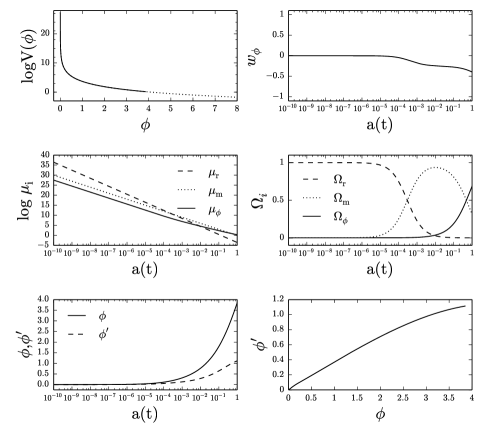
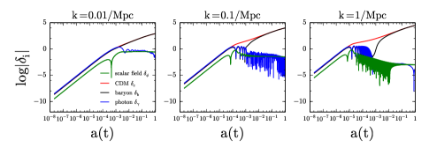
Figure 1: Background (top six panels) and perturbation (bottom three panels for three different scales) evolutions for an inverse power-law potential in Eq. (1). We take $\alpha=6$ for the background. As the initial conditions we use Eqs. (4) and (5) for the background, and Eqs. (21)-(24) for perturbations in the CCG. In the $\phi-V(\phi)$ diagram, the shape of the potential is indicated by the dotted line, and the real evolution till $a_{0}=1$ is indicated by the solid line.

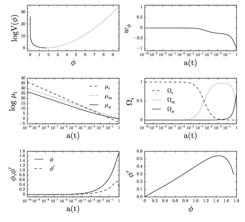
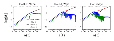
Figure 2: The same as Fig. 1 for a SUGRA potential in Eq. (42). We take $\alpha=6$ and $\lambda=1$ for the background. In this and previous figures, Eq. (24) shows that $\widehat{\delta}_{\phi}$ changes sign at $w={1/9}$.

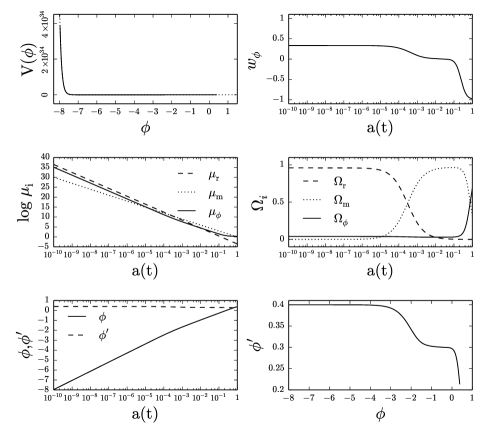
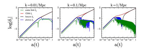
Figure 3: The same as Fig. 1 for a double exponential potential in Eq. (43). We take $\lambda_{1}=10$, $\lambda_{2}=0.1$ and $V_{1}=1$ for the background. In this and next figures, Eq. (41) shows that $\widehat{\delta}_{\phi}$ changes sign at $w={1/9}$.

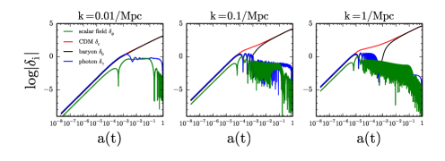
Figure 4: The same as Fig. 1 for AS potential in Eq. (44). We take $\lambda_{1}=10$, $\lambda=10$, $\phi_{0}=-1$ and $A=0.005$ for the background.

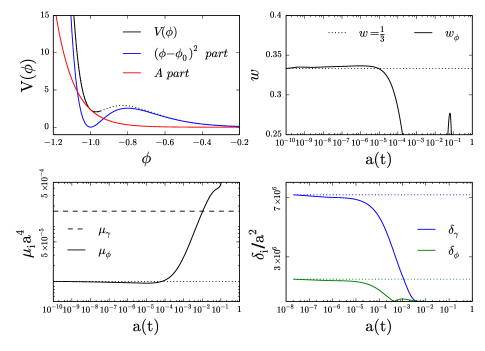
Figure 5: The same model as in Fig. 4, now showing the approximate nature of our solutions in the AS model. Notice the small difference of the $w_{\phi}$, $\mu_{\phi}$, $\delta_{\phi}$ and $\delta_{\gamma}$ compared with the dotted line (the scaling solution) in the early era (till around $a\sim 10^{-5}$). Except for this understandable difference in details our solution is still quite successful.

V Discussion

We presented the perturbation initial conditions for a fluids-field system with two types of scalar field potential in two gauge conditions. The fluids-field system includes an ideal fluid with constant $w$, a minimally coupled scalar field, and a subdominant zero-pressure fluid. The solutions are: for inverse power-law potential, Eqs. (10), (14)-(17) in the $w$CG and Eqs. (21)-(24) in the CCG, and for exponential potential, Eqs. (32)-(36) in the $w$CG and Eqs. (37)-(41) in the CCG.

As we have shown in the previous section the CCG initial conditions for the two type of potentials will have wide applications in the Markov chain Monte Carlo parameter estimation with the scalar field as the dark energy. We have implemented the scalar field in the CAMB CAMB . The CAMB is based on the synchronous gauge with additional fixing of the remnant gauge mode by setting $v_{c}\equiv 0$, and this is the same as the CCG. Thus our perturbation solutions in the CCG are suitable for initial conditions for CAMB supplemented by a scalar field as the dark energy. We will study the role of scalar field as the dark energy in future.

J.H. was supported by Basic Science Research Program through the National Research Foundation (NRF) of Korea funded by the Ministry of Science, ICT and future Planning (No. 2016R1A2B4007964 and No. 2018R1A6A1A06024970). H.N. was supported by National Research Foundation of Korea funded by the Korean Government (No. 2018R1A2B6002466). C.-G.P. was supported by the Basic Science Research Program through the National Research Foundation of Korea (NRF) funded by the Ministry of Education (No. 2017R1D1A1B03028384).

Appendix: Basic equations

We present a complete set of background and scalar-type perturbation equations of multiple component fluids and a scalar field system in a flat Friedmann world model. Our metric and energy-momentum tensor convention is

$$ds^{2}=-a^{2}\left(1+2\alpha\right)d\eta^{2}-2a\chi_{,i}d\eta dx^{i}$$

$$\qquad+a^{2}\left(1+2\varphi\right)\delta_{ij}dx^{i}dx^{j},$$ (45)

$$T^{0}_{0}=-\left(\mu+\delta\mu\right),\quad T^{0}_{i}=-\left(\mu+p\right)v_{,i},$$

$$T^{i}_{j}=\left(p+\delta p\right)\delta^{i}_{j}.$$ (46)

Background equations are

$$H^{2}={8\pi G\over 3}\mu+{\Lambda\over 3},$$ (47)

$$\dot{\mu}+3H\left(\mu+p\right)=0,$$ (48)

where $H\equiv\dot{a}/a$ with an overdot indicating a time derivative based on $t$ with $dt\equiv ad\eta$. In the multiple component case, for individual component, we have

$$\dot{\mu}_{I}+3H\left(\mu_{I}+p_{I}\right)=0,$$ (49)

and

$$\mu=\sum_{J}\mu_{J},\quad p=\sum_{J}p_{J}.$$ (50)

For a MSF we have

$$\ddot{\phi}+3H\dot{\phi}+V_{,\phi}=0,$$ (51)

$$\mu_{\phi}={1\over 2}\dot{\phi}^{2}+V,\quad p_{\phi}={1\over 2}\dot{\phi}^{2}-V.$$ (52)

Ignoring the anisotropic stress, the scalar-type perturbation equations without taking the temporal gauge (slicing) condition are Bardeen-1988 ; HN-2001-scaling

$$\kappa=3H\alpha-3\dot{\varphi}-{\Delta\over a^{2}}\chi,$$ (53)

$$4\pi G\delta\mu+H\kappa+{\Delta\over a^{2}}\varphi=0,$$ (54)

$$\kappa+{\Delta\over a^{2}}\chi-12\pi Ga\left(\mu+p\right)v=0,$$ (55)

$$\dot{\kappa}+2H\kappa+\left(3\dot{H}+{\Delta\over a^{2}}\right)\alpha=4\pi G\left(\delta\mu+3\delta p\right),$$ (56)

$$\varphi+\alpha-\dot{\chi}-H\chi=0,$$ (57)

$$\delta\dot{\mu}+3H\left(\delta\mu+\delta p\right)+\left(\mu+p\right)\left(3H\alpha-\kappa-{\Delta\over a}v\right)$$

$$\qquad=0,$$ (58)

$${1\over a^{4}}\left[a^{4}\left(\mu+p\right)v\right]^{\displaystyle\cdot}={1\over a}\left[\delta p+\left(\mu+p\right)\alpha\right].$$ (59)

For each component, the conservation equations are

$$\delta\dot{\mu}_{I}+3H\left(\delta\mu_{I}+\delta p_{I}\right)$$

$$\qquad+\left(\mu_{I}+p_{I}\right)\left(3H\alpha-\kappa-{\Delta\over a}v_{I}\right)=0,$$ (60)

$${1\over a^{4}}\left[a^{4}\left(\mu_{I}+p_{I}\right)v_{I}\right]^{\displaystyle\cdot}={1\over a}\left[\delta p_{I}+\left(\mu_{I}+p_{I}\right)\alpha\right],$$ (61)

and we have

$$\delta\mu=\sum_{J}\delta\mu_{J},\quad\delta p=\sum_{J}\delta p_{J},$$

$$v={\sum_{J}(\mu_{J}+p_{J})v_{J}\over\sum_{K}(\mu_{K}+p_{K})}.$$ (62)

For the scalar fields we have

$$\delta\ddot{\phi}+3H\delta\dot{\phi}-{\Delta\over a^{2}}\delta\phi+V_{,\phi\phi}\delta\phi$$

$$\qquad=2\ddot{\phi}\alpha+\dot{\phi}\left(\dot{\alpha}+3H\alpha+\kappa\right),$$ (63)

and

$$\delta\mu_{\phi}=\dot{\phi}\delta\dot{\phi}-\dot{\phi}^{2}\alpha+V_{,\phi}\delta\phi,$$

$$\delta p_{\phi}=\dot{\phi}\delta\dot{\phi}-\dot{\phi}^{2}\alpha-V_{,\phi}\delta\phi,\quad v_{\phi}={1\over a}{\delta\phi\over\dot{\phi}}.$$ (64)

References

(1)
V. Sahni, A. Starobinsky, Int. J. Mod. Phys. D 9, 373 (2000);
P.J.E. Peebles, B. Ratra RMP 75, 559 (2003);
E.J. Copeland, M. Sami, S. Tsujikawa, Int. J. Mod. Phys. D 15, 1753 (2006);
L. Amendola, S. Tsujikawa, Dark Energy (Cambridge Univ. Press, 2010).
(2)
J. Hwang, H. Noh, PRD 64, 103509 (2001).
(3)
A. Lewis, A. Challinor, A. Lasenby, Astrophys. J. 538, 473 (2000) ;
A.M. Lewis, Ph.D. thesis, University of Cambridge (2000);
C. Howlett, A. Lewis, A. Hall, and A. Challinor, JCAP 04, 027 (2012);
A. Lewis, CAMB Notes, http://cosmologist.info/notes/CAMB.pdf;
CAMB homepage in A. Lewis and A. Challinor, http://camb.info/ (1999).
(4)
P.J.E. Peebles, B. Ratra, ApJ 325, L17 (1988).