IQ-Collaboratory 1.1: the Star-Forming Sequence of Simulated Central Galaxies

Abstract

A tightly correlated star formation rate–stellar mass relation of star forming galaxies, or star-forming sequence (SFS), is a key feature in galaxy property-space that is predicted by modern galaxy formation models. We present a flexible data-driven approach for identifying this SFS over a wide range of star formation rates and stellar masses using Gaussian mixture modeling (GMM). Using this method, we present a consistent comparison of the $z{=}0$ SFSs of central galaxies in the Illustris, EAGLE, and Mufasa hydrodynamic simulations and the Santa Cruz semi-analytic model (SC-SAM), alongside data from the Sloan Digital Sky Survey. We find, surprisingly, that the amplitude of the SFS varies by up to ${\sim}0.7\,\mathrm{dex}$ (factor of ${\sim}5$) among the simulations with power-law slopes range from 0.7 to 1.2. In addition to the SFS, our GMM method also identifies sub-components in the star formation rate–stellar mass relation corresponding to star-burst, transitioning, and quiescent sub-populations. The hydrodynamic simulations are similarly dominated by SFS and quiescent sub-populations unlike the SC-SAM, which predicts substantial fractions of transitioning and star-burst galaxies at stellar masses above and below $10^{10}M_{\sun}$, respectively. All of the simulations also produce an abundance of low-mass quiescent central galaxies in apparent tension with observations. These results illustrate that, even among models that well reproduce many observables of the galaxy population, the $z{=}0$ SFS and other sub-populations still show marked differences that can provide strong constraints on galaxy formation models.

1 Introduction

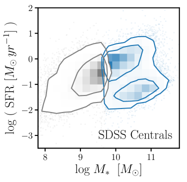
Large galaxy surveys of the past decade such as the Sloan Digital Sky Survey (SDSS; York et al., 2000), have firmly established the major trends of galaxies in the local universe. Galaxies broadly fall into two populations: quiescent galaxies with little star formation that are red in color with elliptical morphologies and star forming galaxies with significant star formation that are blue in color with disk-like morphologies (Kauffmann et al. 2003; Blanton et al. 2003; Baldry et al. 2006; Taylor et al. 2009; Moustakas et al. 2013; see Blanton & Moustakas 2009 and references therein). Star-forming galaxies, furthermore, are found to have a tight relationship between their star formation rates (SFR) and stellar masses placing them on the so-called “star-forming sequence” (hereafter SFS; e.g. Noeske et al., 2007; Daddi et al., 2007; Salim et al., 2007, see also Figure 1).

In fact, this sequence of star-forming galaxies is found in observations well beyond the local universe out to $z>2$ (Wang et al., 2013; Leja et al., 2015; Schreiber et al., 2015). But more than its persistence, the SFS plays a crucial role in characterizing the evolving galaxy population. Although its importance is contested (Kelson, 2014; Abramson et al., 2016), the most dramatic transformations of galaxies over the past $10\,\mathrm{Gyr}$ can be described by the SFS. For instance, the decline in the number density of massive star-forming galaxies and the accompanying growth in number density of quiescent galaxies reflects the cessation of star formation in star-forming galaxies migrating off of the SFS (Blanton, 2006; Borch et al., 2006; Bundy et al., 2006; Moustakas et al., 2013). Similarly, the cosmic decline in star formation (Hopkins & Beacom, 2006; Behroozi et al., 2013a; Madau & Dickinson, 2014) reflects the overall decline of star formation of the SFS (Schreiber et al., 2015).

Galaxy formation models qualitatively reproduce the SFS and similar global relations of galaxy properties at $z\sim 0$ and provide insights into the key physical processes governing those relations (e.g. Vogelsberger et al. 2014; Genel et al. 2014; Schaye et al. 2015; Somerville et al. 2015; Davé et al. 2017a; for a recent review see Somerville & Davé 2015). These hydrodynamic and semi-analytic simulations each seek to capture the complex physics of gas heating and cooling, star formation, stellar feedback, chemical evolution, black hole formation and evolution, and feedback from active galactic nuclei (AGN) using their distinct sub-grid model prescriptions. Many works have already compared the simulations considered in this paper to observations of, for example, galaxy masses, colors, and star formation rates (e.g. Vogelsberger et al., 2014; Genel et al., 2014; Torrey et al., 2014; Sparre et al., 2015; Schaye et al., 2015; Bluck et al., 2016; Davé et al., 2017a; Somerville & Davé, 2015). These works, however, primarily focus on comparing one specific simulated galaxy sample to one or a few observational datasets. Extending such comparisons to include multiple simulations, observations, and a consistent framework for comparing the data-sets would allow us to make detailed comparison of the different sub-grid models and thereby provide key constraints on the physics that govern galaxy formation and evolution.

The SFS, given its prominence, naturally presents itself as a key feature in the data-space of galaxy properties to compare across both observations and simulations. Moreover, with the important role it plays in characterizing the evolving galaxy population, the SFS provides a way to interpret and understand the different galaxy subpopulations and the processes that create them. Two main challenges lie in conducting a meaningful comparison of the SFS. First is the lack of a flexible and data-driven method for identifying the SFS across different datasets. In fact, inconsistencies in how the SFS is identified have incorrectly led to agreement among simulations and observations (e.g. Somerville & Davé, 2015, see Appendix A). The other challenge is the difference in methodology for deriving galaxy properties (such as SFR, $M_{*}$), which even for the same data-set dramatically impacts the SFS (e.g. Speagle et al., 2014). In this paper we address the first challenge by presenting a flexible, data-driven method for identifying the SFS. We then use this method to compare the $z=0$ central galaxy populations of the Illustris, EAGLE, and Mufasa hydrodynamic simulations and the Santa Cruz Semi-Analytic Model (SC-SAM), alongside observations from SDSS.

In Section 2, we describe the data-sets from simulations and observations and how we specifically select our galaxy sample. Then in Section 3, we describe how we identify the SFS with a data-driven approach using Gaussian mixture modeling. We present the resulting SFSs from the simulations and observations in Section 4 and compare the galaxy populations of the simulations and observations. Finally, we conclude and summarize the results of our comparison in Section 5. This paper is the first in a series, initialized by the IQ (Isolated & Quiescent)-Collaboratory, which aims to improve our understanding of quenching processes by comparing isolated star-forming and quiescent galaxies in simulations and observations. This first project in the IQ-Collaboratory focuses on the star-forming and quiescent galaxy populations at $z\sim 0$. Additional projects will focus on galaxy populations at the peak of cosmic star formation (Choi et al. in prep.), and the gas content of star-forming and quenched galaxies (Emerick et al. in prep.). In the subsequent paper of this project (IQ 1.2), we will address the challenges in measured galaxy properties by forward modeling mock spectra of simulated galaxies and measuring their properties in the same manner as observations (Starkenburg et al. in prep).

Figure 1: Star-forming central galaxies in the SDSS have a well-defined relationship between their SFRs and stellar masses, placing them on the “star-forming sequence”. Our SDSS central galaxy sample is derived from a volume-limited sample from Tinker et al. (2011) at $M_{*}>10^{9.7}M_{\sun}$ (blue) and a low luminosity sample from Geha et al. (2012) at $M_{*}<10^{9.7}M_{\sun}$ (gray) described in Section 2.5.

2 The Galaxy Samples

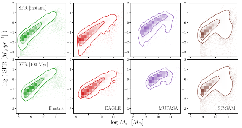
In this work, our main focus is to compare simulated central galaxies from four large-scale cosmological simulations: three hydrodynamic (Illustris, EAGLE, and Mufasa) and one semi-analytic (SC-SAM). A consistent comparison requires consistently defined galaxy properties across the simulations. For all of the simulated galaxies we derive their stellar masses using the same definition and their SFRs on two timescales: instantaneous and averaged over $100\,\mathrm{Myr}$. SFR on these timescales correspond to $H{\alpha}$ and $UV$ based SFR measurements, which represent the formation of young stars with ages ${\lesssim}10\,\mathrm{Myr}$ and star formation in the last ${\sim}100\,\mathrm{Myr}$ (e.g. Kennicutt & Evans, 2012), respectively. We use instantaneous SFR, instead of SFR averaged over $10\,\mathrm{Myr}$, to minimize resolution effects in hydrodynamic simulations on such short timescales (Appendix C).

In the hydrodynamic simulations, we derive the instantaneous SFRs from the rate of star formation in the dense and cold gas and the $100\,\mathrm{Myr}$ averaged SFRs from the ages, or formation times, of star particles in the galaxies. For the semi-analytic model, we derive the instantaneous SFR using the Kennicutt-Schmidt relation for molecular hydrogen (based on Bigiel et al., 2008) and the derived H₂ surface density in radial bins. We derive the $100\,\mathrm{Myr}$ averaged SFRs from the total stellar mass formed in the galaxies, which is outputted from the model every $10\,\mathrm{Myr}$. Meanwhile, for the stellar mass of the simulated galaxies, we use the total stellar mass within the host halos, discounting the stellar mass in any subhalo within the halo. While stellar masses defined within some effective radius is better suited for comparison to observations, we use the total stellar mass within the halo because different sub-grid models can significantly alter galaxy sizes. Furthermore, although halos are identified differently in the simulations, nearly all the stellar mass is in the center of halos. Therefore, the stellar masses are consistently defined among the simulations.

From the SFRs and stellar masses, we derive the specific-SFRs of the galaxies as $\log\,\mathrm{SSFR}=\log\,\mathrm{SFR}-\log\,M_{*}$. Due to the numerical and resolution effects a significant number of galaxies in the hydrodynamic simulations have $100\,\mathrm{Myr}$ averaged “SFR$=0$”, when their SFRs are below the resolution limit of the simulations. We consider these galaxies to have “unmeasurably low SFRs”. For the instantaneous SFRs and both SFRs for the SC-SAM, we analogously consider $\log\,\mathrm{SFR}<-4\ M_{\sun}\mathrm{yr}^{-1}$ as "unmeasureably low SFR". We discuss in Appendix C, how we treat the effect of spatial, mass, and temporal resolution of the simulations, which can impact SFR, in further detail.

In the rest of this section we provide a brief description of the Illustris, EAGLE, Mufasa, and SC-SAM simulations and each of their key sub-grid and feedback prescriptions. In addition, we briefly describe the SDSS galaxy sample, which we include for reference in Section 2.5. Lastly, we describe how we consistently identify central galaxies among the simulations and observations in Section 2.6.

2.1 Illustris

The Illustris simulation (Vogelsberger et al. 2014; Genel et al. 2014; public data release Nelson et al. 2015) evolves a cosmological volume of $(106\ \rm{Mpc})^{3}$ with a uniform baryonic mass resolution of $1.26\times 10^{6}M_{\sun}$ using the Arepo moving-mesh code (Springel, 2010). It employs sub-grid models for star-formation (Springel & Hernquist, 2003), Bondi-like supermassive black hole (SMBH) accretion, a phenomenological model for galactic winds (Oppenheimer & Davé, 2006), and two main modes for energy injection from SMBHs (see Vogelsberger et al., 2013). When gas accretion onto the SMBH occurs at Eddington ratios $>0.05$, thermal energy is injected continuously in the local environment of the SMBH. At lower accretion rates, the energy injection occurs in bursts at large distances from the SMBH, generating hot bubbles in the intracluster medium (Sijacki et al., 2007). Previous works discussing aspects of the SFS and/or quenching in Illustris include Genel et al. (2014); Vogelsberger et al. (2014); Sparre et al. (2015); Bluck et al. (2016); Terrazas et al. (2017).

2.2 EAGLE

The Virgo Consortium’s Evolution and Assembly of GaLaxies and their Environment (EAGLE) project (Schaye et al., 2015; Crain et al., 2015) is a publicly available (McAlpine et al., 2016) suite of cosmological, hydrodynamic simulations of a standard $\Lambda$ cold dark matter universe. Of the simulations, we use L0100Ref, which has a volume of $(100\,\mathrm{comoving\,Mpc})^{3}$ and baryonic mass resolution of $1.81\times 10^{6}M_{\sun}$. It uses Anarchy (Dalla Vecchia et al. in prep.; see also Appendix A of Schaye et al. 2015 and Schaller et al. 2015), which is a modified version of the ${\sc Gadget}$ 3 $N$-body/SPH code (Springel, 2005) that includes modifications to the SPH formulation, time stepping, and sub-grid physics. The sub-grid model for feedback from massive stars and AGN is based on thermal energy injection in the ISM (Dalla Vecchia & Schaye, 2012). The simulations resolve galaxies above $M_{*}>10^{8}M_{\sun}$. The SFR–$M_{*}$ relation and quiescent fractions in EAGLE have been previously discussed in Furlong et al. (2015); Trayford et al. (2015, 2017).

2.3 Mufasa

Mufasa is a hydrodynamic simulation with a box size of $(50\,h^{-1}\ {\rm Mpc})^{3}$ and particle masses of $9.6\times 10^{7}\ M_{\sun}$ and $1.82\times 10^{7}\ M_{\sun}$ for dark matter and baryons, respectively. It uses Gizmo, a code built on Gadget that uses the Meshless Finite Mass hydrodynamics method (Hopkins, 2015) rather than SPH. Mufasa includes star formation via a Kennicutt-Schmidt law based on the molecular hydrogen density as computed using the sub-grid recipe in Krumholz & Gnedin (2011). It also includes two-phase kinetic outflows with scalings as predicted in the Feedback in Realistic Environments (FIRE) simulations (Muratov et al., 2015). Finally, it quenches massive galaxies by keeping all non-self shielded gas within halos above a mass of $M_{q}>(1+0.48z)\,10^{12}M_{\sun}$ near the halos’ virial temperature (Gabor & Davé, 2015; Mitra et al., 2015). The stellar mass function, gas and metal content of galaxies, and color-mass diagram of Mufasa have been previously discussed in Davé et al. (2016, 2017a, 2017b).

2.4 Santa Cruz Semi-Analytic Model

The ‘Santa Cruz’ SAM (SC-SAM) is a semi-analytic model run on merger trees from a ($100$ comoving Mpc/$h$)³ subvolume of the Bolshoi–Planck dark matter only $N$-body simulations (Rodríguez-Puebla et al., 2016). The Bolshoi–Planck simulations have particle masses of $1.5\times 10^{8}M_{\sun}$. The model includes schematic prescriptions for gas heating and cooling, multi-phase gas partitioning, star formation, chemical evolution, feedback from stars, supernovae and SMBHs, the sizes of galactic disks and bulges, and merger-induced starbursts and structural transformations. The SC-SAM was first presented in Somerville & Primack (1999) and Somerville et al. (2001), with significant updates described in Somerville et al. (2008b, a, 2012); Porter et al. (2014); Popping et al. (2014); Somerville et al. (2015). In this work, we use the version of the SC-SAM described in Popping et al. (2014) and Somerville et al. (2015), which includes the Gnedin & Kravtsov (2011) recipe for partitioning multi-phase gas into HI, H₂ and HII based on the dark matter resolution limit, we focus our analysis on halos with $M_{h}{>}10^{11}M_{\sun}$. Since this roughly corresponds to $M_{*}{\sim}10^{8.5}M_{\sun}$ at $z\sim 0$, we impose a conservative cut of $M_{*}>10^{8.8}M_{\sun}$. The properties of the SC-SAM galaxy population, such as the quiescent fraction have been previously discussed in Brennan et al. (2015); Somerville et al. (2015); Somerville & Davé (2015); Brennan et al. (2017); Pandya et al. (2017).

2.5 Observed SDSS Galaxies

As a reference to our comparison of the simulated galaxies, we include SDSS galaxies from two samples: a $M_{*}{>}10^{9.7}M_{\sun}$ Data Release 7 (DR7; Abazajian et al., 2009) sample and a $M_{*}<10^{9.7}M_{\sun}$ Data Release 8 (DR8; Aihara et al., 2011) sample (blue and gray in Figure 1). At high masses, we use the volume-limited galaxy sample from Tinker et al. (2011) constructed from the NYU Value-Added Galaxy Catalog (VAGC; Blanton et al., 2005). It has $M_{r}-5\log(h)<-18$ and is complete for $M_{*}>10^{9.7}M_{\sun}$. For further details, we refer readers to Tinker et al. (2011); Wetzel et al. (2013); Hahn et al. (2017).

At lower stellar masses, we use the isolated dwarf galaxy sample of Geha et al. (2012) from the NASA Sloan Atlas (NSA), a reprocessing of SDSS DR8. The NSA is optimized for low-luminosity objects and relies on the improved background subtraction technique of Blanton et al. (2011). The catalog extends to $z\approx 0.055$ and includes re-calibrated spectroscopy (Yan, 2011; Yan & Blanton, 2012) with much smaller errors.

For both SDSS subsamples, the stellar masses are estimated using the Blanton & Roweis (2007) $\mathtt{kcorrect}$ code, which assumes a Chabrier (2003) IMF. The SFRs are from the current release of Brinchmann et al. (2004), where they are derived using the Bruzual A. & Charlot (1993) model with the Charlot & Fall (2000) dust prescription and CLOUDY (version C90.04; Ferland, 1996) emission line modeling. For galaxies classified as having an AGN or a composite spectrum, the SFR is measured from the $D_{n}4000$ index (Balogh et al., 1998). Additionally, for star-forming galaxies that have low S/N spectra, the SFR is derived from the $H{\alpha}$ luminosity (Brinchmann et al., 2004). We emphasize that SSFRs $\lesssim 10^{-12}\mathrm{yr}^{-1}$ should only be considered upper limits to the true value (Salim et al., 2007). Given the disparate methods used for the SFR measurements, the SFRs in the SDSS sample do not entirely correspond to either the instantaneous or $100\,\mathrm{Myr}$ averaged SFRs of the simulations. Consequently, in this work we compare the simulations on both timescales and refrain from detailed comparisons to SDSS.

2.6 Identifying Central Galaxies

Measurements of the quiescent fraction (e.g. Baldry et al., 2006; Peng et al., 2010; Hahn et al., 2015) and star formation quenching timescale (Wetzel et al., 2013; Hahn et al., 2017) suggest, whether a galaxy is a satellite or central galaxy influences its star formation rate. There may also be significant differences between the SFSs of central versus satellite galaxies (Wang et al., 2018). In this paper we focus solely on the central galaxies, which constitute the majority of massive galaxies ($M_{*}>10^{9.5}M_{\sun}$) at $z\sim 0$.

Central classification, despite its importance, is often heterogeneously defined in the literature. Among simulations, the classification depends on the definition of halo properties, and thus on the underlying halo finders. EAGLE and Illustris use $\mathtt{SUBFIND}$ (Springel et al., 2001), where halos are defined as locally overdense, gravitationally bound (sub)structures within a connected region selected through a friend-of-friends (FOF; Davis et al., 1985) group finder. Mufasa and SC-SAM, meanwhile, use $\mathtt{ROCKSTAR}$ (Behroozi et al., 2013b), which defines halos using a hierarchical phase-space based FOF technique and seeks to maximize the consistency of the halo through time. In addition, these central classifications also use information of the underlying dark matter — information not available in observations. Therefore, we identify central galaxies in all simulations consistently using the Tinker et al. (2011) group finder, designed to identify satellite/centrals in observations.

The Tinker et al. (2011) group finder is a halo-based algorithm that uses the abundance matching ansatz to iteratively assign halo masses to groups. It assigns a tentative halo mass to each galaxy by matching the abundance of the objects. Then starting with the most massive galaxy, nearby lower mass galaxies are assigned a probability of being a satellite. Once all the galaxies are assigned to a group, the halo masses of the central galaxies are updated by abundance matching with the total stellar mass in the groups. This entire process is repeated until convergence. In the resulting catalog, every group contains one central galaxy, which by definition is the most massive, and a group can contain zero, one, or many satellites. For a detailed description we refer readers to Tinker et al. (2011); Wetzel et al. (2012).

Overall, we find good agreement between the central classifications of the group finder with respect to that of the simulations with purities of $99\%,93\%,84\%$, and $97\%$ and completenesses of $86\%$, $89\%$, $91\%$, and $85\%$ for the Illustris, EAGLE, Mufasa and SC-SAM simulations respectively. Differences in the purity and completeness for the simulations is likely due to the different halo finders used in the simulations. We find no significant stellar mass dependence in the purities. As expected from the high purity and completeness, when we perform our analysis using the centrals and identified by the dark matter halos, we find no significant differences. In the next section, we proceed to fitting the star-forming sequence of simulated central galaxies.

Figure 2: The SFR–$M_{*}$ relations of central galaxies from the Illustris (green), EAGLE (red), and Mufasa (purple) hydrodynamic simulations and the SC-SAM (brown) at $z=0$. The top panels use instantaneous SFRs while the bottom panels use SFRs averaged over $100\,\mathrm{Myr}$. The contours in each panel mark the $68\%$ and $95\%$ confidence intervals of the SFR–$M_{*}$ distribution. We describe the simulations and how we derive consistent SFRs and stellar masses in Section 2. The SFR–$M_{*}$ relations reveal star-forming sequences in all of the simulations.

Figure 3: We illustrate our GMM based method for identifying the SFS of Illustris central galaxies in two stellar mass bins highlighted on the SFR–$M_{*}$ relation of the left panel: $10.4<\log\,M_{*}<10.6$ and $11.0<\log\,M_{*}<11.2$. We compare the SSFR distributions, $p(\log\,\mathrm{SSFR})$, in the two stellar mass bins to their best-fit GMMs (right panels). The $p(\log\,\mathrm{SSFR})$ in the center panel is best described by a GMM with three components (orange, green, and blue) while the $p(\log\,\mathrm{SSFR})$ in the right panel is best described by a GMM with two components (orange and blue). The SFS components of the best-fit GMMs are plotted in blue. Our GMM method provides a flexible and data-driven method of identifying the SFS in a wide variety of SSFR distributions without hard assumptions or cuts to the sample.

3 Identifying the Star-Forming Sequence

We present the SFR–$M_{*}$ relation of central galaxies from the observations and simulations of Section 2 in Figures 1 and 2. For both instantaneous and $100\,\mathrm{Myr}$ SFRs (top/bottom), in both simulations and observations, and over four orders of magnitude in SFR and stellar mass, the SFR and $M_{*}$ of star-forming galaxies lie on a well-defined SFS. Despite its universality, in detail, the different datasets give rise to different SFR–$M_{*}$ distributions, which makes the SFS difficult to consistently and meaningfully quantify. So far in the literature, a wide variety of fitting methods has been applied to data — even in a single comparison (see Appendix A). For example, in Lee et al. (2015) and some of the fits in Somerville & Davé (2015) the SFS is fit using median $\log\,\mathrm{SFR}$s of galaxies after some color-color or SSFR cut to the sample. Other SFSs in Somerville & Davé (2015) are fit using the median $\log\,\mathrm{SFR}$s of the entire sample. Bluck et al. (2016) fit the SFS using median $\log\mathrm{SFR}$s of low mass galaxies ($M_{*}<10^{10}M_{\sun}$) and extrapolate to higher masses. Other recent works in the literature have opted for more sophisticated methods such as fitting a three-component Gaussian (Bisigello et al., 2018) or a zero-inflated negative binomial distribution (Feldmann, 2017).

All of these methods require arbitrary assumptions or hard cuts to the sample. More importantly, for such methods, different assumptions or cuts produce different SFSs and inconsistent assumptions and cuts can result in misleading SFS comparisons (Appendix A). Identifying the SFS also requires flexibility in accounting for the different features in the galaxy property space over a wide SFR or $M_{*}$ range and in different simulations and observations. In an effort to better fit the SFS from a wide variety of SFR–$M_{*}$ distributions and to relax the assumptions and cuts imposed on the data, we present a flexible and data-driven method for identifying the SFS that makes use of Gaussian Mixture Models.

3.1 Using Gaussian Mixture Models

Gaussian mixture models (hereafter GMM), and mixture models in general, provide a probabilistic way of describing the distribution of a population by identifying subpopulations from the data (Press et al., 1992; McLachlan & Peel, 2000). Besides their extensive use in machine learning and statistics, GMMs have also been used in a wide range of astronomical analyses (e.g. Bovy et al., 2011; Lee et al., 2012; Taylor et al., 2015). Since identifying the subpopulation of star-forming galaxies from the overall galaxy population is equivalent to identifying the SFS, GMMs provides a well-motivated, data-driven, and effective method to tackle the problem.

A GMM, more precisely, is a weighted sum of $k$ Gaussian component densities

$$\hat{p}(x;\bm{\theta})=\sum\limits_{i=1}^{k}\pi_{i}\,\mathcal{N}(x;\bm{\theta}_{i}),$$ (1)

which can be used to estimate the density. The weights, $\pi_{i}$, mean, and variance $\bm{\theta}_{i}=\{\mu_{i},\sigma_{i}\}$ of the components are free parameters. For a given data set $\{x_{1},...,x_{n}\}$, these parameters are most commonly estimated through the expectation-maximization algorithm (EM; Dempster et al., 1977; Neal & Hinton, 1998).

Starting with randomly assigned $\bm{\theta}_{i}^{0}$ to the $k$ GMM components, the EM algorithm iterates between two steps. First, for every data point, $x_{i}$, the algorithm computes for a probability of $x_{i}$ being generated by each GMM component. These probabilities act as assignment weights to each of the components. Next, based on these weights, $\bm{\theta}_{i}^{t}$ of the components are updated to $\bm{\theta}_{i}^{t+1}$ to maximize the likelihood of the assigned data. $\pi_{i}$ are also updated by summing up the assignment weights and normalizing the sum by the total number of data points. These steps are repeated until $p(\{x_{1},...,x_{n}\};\bm{\theta}_{t})$ converges. Instead of starting with randomly assigning $\bm{\theta}_{i}^{0}$, we initiate our EM algorithm using a $k$-means clustering algorithm (Lloyd, 1982), more specifically we use the $k$-$\mathtt{means}$++ algorithm (Arthur & Vassilvitskii, 2007).

For actually identifying the SFS, we first divide the galaxy sample into stellar mass bins of some width $\Delta\log M_{∗}$. In this paper we use bins of $\Delta\log M_{*}=0.2\ \mathrm{dex}$; however, this choice does not significantly impact the final SFS. For each stellar mass bin, if there are more than $N_{\mathrm{thresh}}{=}100$ galaxies in the bin, we fit the SSFR distribution using GMMs with $k{=}1$ to 3 components with parameters determined from the EM algorithm described above. For the SDSS galaxy sample and the hydrodynamic simulations, even when we allow for more than 3 components, the best-fit GMMs have $k\leq 3$. Hence, the choice of $k\leq 3$ does not significantly impact the results of this work. Out of the three ($k\leq 3$) GMMs, we select the one with the lowest Bayesian Information Criteria (BIC; Schwarz, 1978) as our “best-fit” model. BIC is often used in conjunction with GMMs (e.g. Leroux, 1992; Roeder & Wasserman, 1997; Fraley & Raftery, 1998; Steele & Raftery, 2010) and also more generally for model selection in astronomy (e.g. Liddle, 2007; Broderick et al., 2011; Vakili & Hahn, 2016). In addition to the likelihood, BIC introduces a penalty term for the number of parameters in the model. This way, using BIC not only finds a good fit to the data, but it also addresses the concern of over-fitting.

Given the best-fit GMM, we next identify the SFS components in each $\log M_{*}$ bin. We start from the lowest $\log M_{*}$ bin, where we take the component with the largest weight as the SFS component. Then in the next higher $\log M_{*}$ bin we identify the component with the largest weight. If this component has a mean within $0.5\,\mathrm{dex}$ of the previous lower $\log M_{*}$ bin SFS component mean, we identify this component as the SFS. Otherwise, we discard it and determine whether the component with the next highest weight is within $0.5\,\mathrm{dex}$ of the previous SFS component mean. We repeat this until we either identify a SFS component or, if no component is within $0.5\,\mathrm{dex}$ of the previous SFS component mean, conclude that no SFS component is in the $\log M_{*}$ bin. We repeat this procedure recursively for all the $\log M_{*}$ bins. This scheme takes advantage of the bimodality in the SSFR distributions and assumes that the SFS forms a relatively continuous sequence. In Appendix B, we present a detailed comparison of the GMM fits to the SSFR distributions of the simulations and discuss the advantages of our method in further detail.

In Figure 3, we illustrate our GMM based method for identifying the SFS of the Illustris central galaxies in two stellar mass ranges highlighted in the left panel: $10.4<\log\,M_{*}<10.6$ (center) and $11.0<\log\,M_{*}<11.2$ (right). For the two stellar mass bins, we compare the SSFR distributions of the bins to the components of the best-fit GMMs derived from our method. The SFS components of the best-fit GMMs are plotted in blue. The SSFR distribution of the center panel is best described by a GMM with three components while the SSFR distribution in the right panel is best described by a GMM with only two components. These comparisons highlights the flexibility and effectiveness of our method in identifying the SFS for different SSFR distributions. Our code for identifying the SFS makes use of the following software: astroML (Vanderplas et al., 2012), astropy (Astropy Collaboration et al., 2013; Collaboration et al., 2018), matplotlib (Hunter, 2007), numpy (Van Der Walt et al., 2011), scipy (Jones et al., 2001), and scikit-learn (Pedregosa et al., 2011). All of the code is publicly available at https://github.com/changhoonhahn/LetsTalkAboutQuench.

Figure 4: The SFSs of the central galaxies in the Illustris, EAGLE, Mufasa, and SC-SAM simulations as identified by our GMM based method (Section 3). The SFSs above are identified from the instantaneous SFR–$M_{*}$ relation. The uncertainties of the SFSs are derived using bootstrap resampling and marked by the error bars. For reference, we include the SFS of the SDSS sample in the top right panel and the bottom right panel (black). When we compare the SFSs of the simulations we find that they have significantly different slopes and their amplitudes vary by up to ${\sim}0.7\,\mathrm{dex}$, factor of ${\sim}5$ (bottom right).

Figure 5: Same as Figure 4 but for $100\,\mathrm{Myr}$ SFR. As in Figure 4, the SFSs of the simulations have significantly different slopes and vary in amplitude by up to ${\sim}0.7\,\mathrm{dex}$, factor of ${\sim}5$.

Figure 6: The power-law fits to the SFSs of the Illustris (green), EAGLE (red), Mufasa (purple), and SC-SAM (brown) simulations highlight the significant differences in the slopes of the SFSs. We use instantaneous SFR and $100\,\mathrm{Myr}$ SFR in the left and right panels respectively. For reference, we include the fit to the SDSS SFS (black dotted). We list the best-fit parameters in Table 4.1. For a consistent comparison, we fit the Mufasa SFS below $\log\,M_{*}<10.5$, due to its high stellar mass turnover.

4 Results

4.1 SFS of simulated galaxies

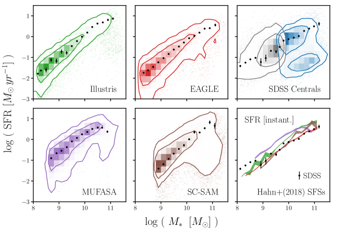
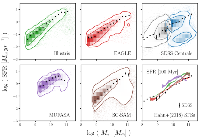
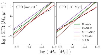
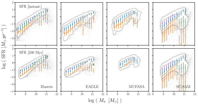
Now using our GMM based method from above, we can identify the SFSs of the simulated central galaxies from Section 2. We present the best-fit SFSs of the simulated galaxies from the Illustris, EAGLE, Mufasa, and SC-SAM simulations for the instantaneous and $100\,\mathrm{Myr}$ SFR timescales in Figures 4 and 5, respectively. In each simulation, for both SFR timescales, the best-fit SFS is in good agreement with the underlying SFR-$M_{*}$ distribution as described by the contour and 2D histogram. However, when we compare the best-fit SFSs of the simulations to each another, we find that they have significantly different slopes and their amplitudes vary by up to $\,{\sim}0.7\,\mathrm{dex}$ (factor of ${\sim}5$) for both the instantaneous and $100\,\mathrm{Myr}$ SFR timescales (bottom right panels of Figures 4 and 5).

The uncertainties for the best-fit SFSs in Figures 4 and 5 are derived from bootstrap resampling (Efron, 1979) in each stellar mass bin. These uncertainties do not account for cosmic variance. Also, they correspond to the uncertainties of the means of the SFS GMM component, which is only one of the parameters in the GMM, and do not account for the correlations other parameters of the GMM in Eq. 1. Our SFS uncertainties are estimated similarly to the cluster red sequence fits in Hao et al. (2009), which use an “error-corrected” GMM that involves bootstrap resampling. Hao et al. (2009), however, use their method to estimate the mean of their GMM component, rather than to estimate its uncertainty.

Using the SFSs we identified, we can now parameterize it to some functional form as often done in the literature — e.g. power-law (Speagle et al., 2014) or broken power-law (Lee et al., 2015). With little evidence of a turnover in the SFS in most of simulations, we fit a power-law of the form

$$\log\,\mathrm{SFR}_{\mathrm{MS}}=m\,(\log\,M_{*}-10.5)+b$$ (2)

to the SFSs in Figure 6. Unlike the SFS of other simulations, the SFSs for Mufasa have a significant turnover at $M_{*}{\sim}10^{10.5}M_{\sun}$. This turnover is not caused by misidentification of the SFS or some systematic effect in the GMM fitting. Instead, the turnover is due to the halo mass dependent quenching prescription in Mufasa (Section 2.3), which causes a sharper cut-off in the SFS, unlike the other more self-consistent AGN feedback models. We focus on the power-law portion of the Mufasa SFS and fit Eq. 2 below the turnover ($M_{*}{<}10^{10.5}M_{\sun}$).

The best-fit (least squares) power-law parameters (Table 4.1 and Figure 6) highlight the significant differences in the slope of the SFSs. Among our simulations, $m$ ranges from sub-linear in Mufasa ($0.75$) to super-linear in SC-SAM ($1.17$). Various sub-grid models (e.g. ISM, star formation, stellar and AGN feedback) can influence the slope and normalization of SFSs in the simulations. To resolve the underlying cause behind the difference in SFSs, would require a detailed comparison of the different sub-grid parameters and prescriptions. While such a comparison is beyond the scope of this paper, the discrepancies we find in the SFSs provide constraints on galaxy formation models. Furthermore, although a detailed comparison with observations is complicated by the differences in how SFR is defined in simulations versus observations, we include in Figure 6 the power-law fit to the SFS of the SDSS central galaxies (black dotted). Compared to the SFSs of the simulations, SFS in SDSS has a significantly a lower slope: $m=0.69$. As a result, the SFSs of the simulations are scattered around the SDSS SFS below $M_{*}{\sim}10^{10}M_{\sun}$, but have higher amplitudes than the SDSS SFS above $M_{*}{\sim}10^{10}M_{\sun}$. This is also apparent in the bottom right panel comparisons of Figures 4 and 5.

The differences we find among the SFSs of the simulations, also propagate to their cosmic star formation densities. Cosmic star formation density roughly corresponds to the total star formation in the SFS weighted by the stellar mass function (SMF). For Illustris, EAGLE, Mufasa, and SC-SAM, respectively, we find total cosmic star formation densities (including satellites) of $10^{-1.66},10^{-2.22},10^{-1.87}$, and $10^{-1.94}\,M_{\sun}\mathrm{yr}^{-1}\mathrm{Mpc}^{-3}$ using instantaneous SFRs and similarly $10^{-1.68}$, $10^{-2.20}$, $10^{-1.91}$, and $10^{-1.94}\,M_{\sun}\mathrm{yr}^{-1}\mathrm{Mpc}^{-3}$ using $100\,\mathrm{Myr}$ SFRs. The rank order of the densities is different than that of the SFSs due to differences in the SMFs. Although these values are roughly within the uncertainties of observations (Madau & Dickinson, 2014), the difference in the star formation density between Illustris and EAGLE, for example, is greater than $0.5\,\mathrm{dex}$— more than factor of 3.

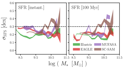
In addition to its position, $\mu_{\mathrm{SFS}}$, the SFS GMM component is also described by $\sigma_{\mathrm{SFS}}$ — the width of the SFS. Using $\sigma_{\mathrm{SFS}}$ derived from the GMM fitting, we can compare the width of the SFS among the simulations (Figure 7). The uncertainties for the widths are calculated through bootstrap resampling in the same way as the SFS uncertainties. Overall, we find little stellar mass dependence in $\sigma_{\mathrm{SFS}}$ for the simulations. For Illustris, EAGLE, Mufasa, and SC-SAM we respectively find $\sigma_{\mathrm{SFS}}{\sim}0.20,0.26,0.25$, and $0.24\,\mathrm{dex}$ for instantaneous SFR and $\sigma_{\mathrm{SFS}}{\sim}0.18,0.20,0.25$, and $0.23\,\mathrm{dex}$ for $100\,\mathrm{Myr}$ SFR (Table 4.1). Although we do not explicitly include the width of the SDSS SFS GMM component due to inconsistencies in the SFRs (Section 2.5), these $\sigma_{\mathrm{SFS}}$ are narrower than the ${\sim}0.3\,\mathrm{dex}$ width measured in observations (e.g. Daddi et al., 2007; Noeske et al., 2007; Salim et al., 2007; Magdis et al., 2012; Whitaker et al., 2012; Speagle et al., 2014). Observational errors, however, will bring the simulated values to closer agreement. Furthermore, the hydrodynamic simulations lack burstiness caused by clustered star formation (and thus feedback) (Sparre et al., 2017). This unresolved variability will also bring the scatter closer to the observed width. We therefore conclude that the width of the SFS from the simulations are in agreement with the observed SFS width.

Table 1: Power-law fit to the SFS of the simulated central galaxies from the Illustris, EAGLE, Mufasa, and SC-SAM simulations.

Star-Forming Sequence power-law fit	width
$\log\,\mathrm{SFR}_{\mathrm{MS}}=m\,(\log\,M_{*}-10.5)+b$
Simulation	$m$	$b$	$\sigma_{\mathrm{SFS}}$ [dex]
Instantaneous SFR
Illustris	1.01 $\pm$ 0.004	0.59 $\pm$ 0.006	0.20
EAGLE	0.91 $\pm$ 0.006	0.23 $\pm$ 0.008	0.26
Mufasa	0.75 $\pm$ 0.014	0.58 $\pm$ 0.011	0.25
Mufasa∗	0.89 $\pm$ 0.020	0.74 $\pm$ 0.020
SC-SAM	1.17 $\pm$ 0.008	0.48 $\pm$ 0.009	0.24
$100\,\mathrm{Myr}$ SFR
Illustris	0.95 $\pm$ 0.006	0.55 $\pm$ 0.008	0.18
EAGLE	0.75 $\pm$ 0.010	0.21 $\pm$ 0.009	0.20
Mufasa	0.38 $\pm$ 0.023	0.36 $\pm$ 0.016	0.25
Mufasa∗	0.97 $\pm$ 0.050	0.83 $\pm$ 0.039
SC-SAM	1.16 $\pm$ 0.008	0.47 $\pm$ 0.009	0.23
SDSS	0.69 $\pm$ 0.008	0.18 $\pm$ 0.007

^∗ power-law fit to the Mufasa SFS below its turnover ($\log\,M_{*}{<}\,10.5$)

One factor that impacts the SFS we identify is the strict lower limit of the $\log\mathrm{SFR}$s caused by the resolution effects in the simulations. This is particularly evident in the $100\,\mathrm{Myr}$ SFR–$M_{*}$ relations of the hydrodynamic simulations of Figure 2 — especially Mufasa. As we describe in Section 2, the $100\,\mathrm{Myr}$ SFRs are calculated using the ages of all star particles in a galaxy. For a galaxy to have star formation (i.e. SFR $>0$), it must at least form one star particle over the last $100\,\mathrm{Myr}$. A single star particle forming over $100\,\mathrm{Myr}$ amounts to a SFR of ${\sim}0.02\ M_{\sun}\mathrm{yr}^{-1}$ for Illustris and EAGLE and ${\sim}0.2\ M_{\sun}\mathrm{yr}^{-1}$ for Mufasa. This resolution limit, ultimately impacts the SFS at $M_{*}{<}10^{8.4}$, $10^{8.4}$, and $10^{9.2}M_{\sun}$ for Illustris, EAGLE, and Mufasa respectively (see Appendix C).

Using our method for identifying the SFS, we are able to conduct a consistent data-driven comparison of the SFSs of simulated central galaxies from the Illustris, EAGLE, Mufasa, and SC-SAM. From this comparison, we find that the amplitudes of the SFSs differ from one another by up to ${\sim}0.7\,\mathrm{dex}$, factor of ${\sim}5$, with significantly different slopes. Furthermore, despite these differences, the SFSs of the simulations have similar widths, consistent with observations.

Figure 7: The width of the SFS, $\sigma_{\mathrm{SFS}}$, for the simulated central galaxies from Illustris, EAGLE, Mufasa, and SC-SAM (green, red, purple, and brown respectively). The uncertainties are estimated using bootstrap resampling in the same way as the SFS uncertainties. The SFS widths in the simulations have little stellar mass dependence and, adding observational measurement errors in SFR, they are roughly consistent with ${\sim}0.3\,\mathrm{dex}$ from observations (black dashed).

Figure 8: Components of the best-fit GMM for the SFR-$M_{*}$ relations of central galaxies in the Illustris, EAGLE, Mufasa, and SC-SAM simulations (left to right). The top and bottom panels use instantaneous SFRs and $100\,\mathrm{Myr}$ SFRs respectively. In each $\log M_{*}$ bin, we mark the SFS component in blue, the low SF component in orange, the intermediate SF component in green, and the component above the SFS in purple. These components loosely correspond to the star-forming, quiescent, transitioning, and star-burst subpopulations. The hydrodynamic simulations have similar subpopulations dominated by the SFS and low SF components. Meanwhile in the SC-SAM, the GMM components reveal broad low SF components that extends out to $\mathrm{SFR}<10^{-4}M_{\sun}\mathrm{yr}^{-1}$, prominent intermediate components at $M_{*}\gtrsim 10^{10}M_{\sun}$, and components above the SFS at $M_{*}\lesssim 10^{10}M_{\sun}$.

Figure 9: Fractional contributions, $\pi_{i}$, of the best-fit GMM components of the central galaxies in Illustris, EAGLE, Mufasa, and SC-SAM (left to right). We highlight the SFS component in blue, the low SF component in orange, galaxies with unmeasurably low SFR in red, the intermediate SF components in green, and the high SF components in purple. We shade the regions below the stellar mass limit set by resolution effects in black (Appendix C). For reference, we include $\pi_{i}$ of the observed SDSS centrals in the rightmost panel. Unlike SDSS or the SC-SAM, we do not find significant high SF components at low $M_{*}$ in the hydrodynamic simulations. Furthermore, treating the components below the SFS as quiescent, we find little $M_{*}$ dependence in the quiescent fraction at $M_{*}<10^{11}M_{\sun}$ unlike observations. In fact, in all of the simulations, we find a significant fraction of quiescent central galaxies at $M_{*}\lesssim 10^{9}M_{\sun}$ contrary to observations.

4.2 Beyond the SFS of Simulated Galaxies

So far we have focused solely on the SFSs of the simulated galaxies — i.e. $\bm{\theta}_{\mathrm{SFS}}=\{\mu_{\mathrm{SFS}},\sigma_{\mathrm{SFS}}\}$ in Eq. 1. Our GMM method, however, also determines $\bm{\theta}_{i}$ of components other than the SFS. These GMM components provide extra features to compare the simulated galaxy samples and also offer interesting insights into the different subpopulations in the simulated galaxy samples. When we examine $\bm{\theta}_{i}$ of all components from our fitting for the simulated galaxies, we find they loosely correspond to galaxy subpopulations typically referred to as quiescent, transitioning, and star-burst (Figure 8). To avoid over-interpreting this correspondence, we refer to the GMM component with the lowest SFR as “low SF” component, the component with SFR in between the SFS and the low SF component as the “intermediate SF” component, and finally the component with higher SFR than the SFS component as the “high SF” component. At a given stellar mass bin, our GMM fits are restricted to $k\leq 3$; hence, the four different components come from different stellar mass bins. In Figure 8, we mark the SFS, low SF, intermediate SF, and high SF in blue, orange, green, and purple respectively.

Examining the GMM components of the hydrodynamic simulations in Figure 8, we find that a few $\log M_{*}$ bins have intermediate SF components in Illustris at $10^{9}M_{\sun}<M_{*}<10^{11}M_{\sun}$. Also a few of the lowest $\log M_{*}$ bins in Illustris and EAGLE have high SF components for the $100\,\mathrm{Myr}$ SFRs. Besides these few bins, however, the central galaxies from the hydrodynamic simulations are dominated by the SFS and low SF components. Furthermore, throughout the stellar mass ranges of the simulations, the low SF components in each of these simulations have relatively constant widths and lie ${\sim}1\,\mathrm{dex}$ below the SFS components.

Unlike the hydrodynamic simulations, however, the low SF components in the SC-SAM span out to $\log\,\mathrm{SFR}{=}{-}4\ M_{\sun}\mathrm{yr}^{-1}$. Furthermore, the intermediate and high SF components are much more prominent in the SC-SAM centrals. At low stellar masses ($M_{*}\lesssim 10^{10}M_{\sun}$) every $\log M_{*}$ bin has a high SF component. The $\log\,\mathrm{SSFR}$ distributions in these bins have extended tails on the higher SFR side of the SFS. Our GMM method, thus, fits high SF components in these $\log M_{*}$ bins (bottom left and center panels of Figures B.1 and B.2). These high SF components and the extended range of low SF components are likely caused by the re-accretion prescription of the SAM (Section 2.7 of Somerville et al. 2008a). A fraction of gas ejected from halos (e.g. from supernovae) is kept in a reservoir, which re-collapses into the halos at a later time and becomes available again for cooling. The rate of this re-accretion depends on the mass of ejected gas, the dynamical time of the halo, and a free parameter degenerate with supernovae feedback parameters. This prescription results in bursty star formation in the SC-SAM galaxies and causes the extended low SF components and the high SF components.

At high stellar masses ($M_{*}\gtrsim 10^{10}M_{\sun}$) every $\log M_{*}$ bin in the SC-SAM has an intermediate component. While the $\log\,\mathrm{SSFR}$ distributions in the bottom right panels of Figures B.1 and B.2 and the BIC values illustrate the benefit of the GMM with an intermediate SF component, these are accentuated by the broader distribution of the low SF population. Despite these differences between the hydrodynamic simulations and the SC-SAM, all of the simulations have a low SF component throughout their stellar mass range, even at $M_{*}<10^{9}M_{\sun}$. We discuss these low $M_{*}$ low SF galaxies in further detail later in this section.

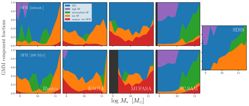
Another set of parameters we infer from our GMM fitting is the weight of the GMM components: $\pi_{i}$ in Eq. 1. These weights correspond to the fractional contribution of the different subpopulations. For example, the weight of the low SF component loosely corresponds to the quiescent fraction (e.g. Borch et al., 2006; Bundy et al., 2006; Iovino et al., 2010; Geha et al., 2012; Hahn et al., 2015). In Figure 9, we present the fractional contribution of the components from our best-fit GMM, as a function of stellar mass: SFS (blue), low SF (orange), intermediate SF (green), and high SF (purple). We also include the fractional contribution of galaxies with unmesurably low SFRs (red; see Section 2). The $\pi_{i}$ have uncertainties, estimated from bootstrap resampling, on the order of ${\sim}0.1$.

For every simulation, a significant fraction of galaxies have unmeasurably low SFRs. In hydrodynamic simulations, a galaxy with unmeasureably low SFR can have an SFR below the resolution limit, or have a “true” $\mathrm{SFR}{=}0$ on the measured timescales (Appendix C). For the SC-SAM, we consider the SFR unmeasurably low when $\log\mathrm{SFR}<{-}4\ M_{\sun}\mathrm{yr}^{-1}$. Therefore, in both hydrodynamic simulations and the SAM, galaxies with unmeasurably low SFR can be considered quiescent. Moreover, we confirm that SFR resolution does not significantly impact the fraction contributions of Figures 9 (see Appendix C and Figure C.3).

The fractional contributions of the GMM components in Figures 9 reveal significant disagreements between the simulated galaxies and trends established from observations— especially the hydrodynamic simulations. For instance, in the hydrodynamic simulations we do not find significant high SF components at low $M_{*}$, unlike in SDSS or SC-SAM. The few $M_{*}$ bins with fractional contributions from high SF components have large bootstrap uncertainties (${\sim}0.2$). Furthermore, if we treat the components below the SFS as quiescent (green, orange and red in Figure 9), we find little stellar mass dependence in the quiescent fraction of the hydrodynamic simulations, unlike the quiescent fraction measurements of isolated SDSS galaxies (Baldry et al., 2006; Peng et al., 2010; Hahn et al., 2015). Meanwhile, at $M_{*}{>}10^{9}M_{\sun}$ the SC-SAM is roughly consistent with SDSS (rightmost panel) and in agreement with previous SC-SAM quiescent fraction comparisons to observations (Brennan et al., 2015, 2017; Pandya et al., 2017).

Furthermore, for some of the hydrodynamic simulations in Figure 9 (Illustris, EAGLE, and Mufasa with $100\,\mathrm{Myr}$ SFRs and EAGLE, and Mufasa instantaneous SFRs) we find surprisingly high quiescent fractions (${\sim}0.4$) at low masses in stark contrast with observations (Baldry et al., 2006; Peng et al., 2010; Hahn et al., 2015). In fact, all the simulations, even the SC-SAM, have non-negligible (${\gtrsim}10\%$) quiescent fraction at $M_{*}{<}10^{9}M_{\sun}$ contrary to the $M_{*}$ lower bound of ${\sim}10^{9}M_{\sun}$ for isolated/central quiescent galaxies we observe in SDSS and established in the literature (e.g. Geha et al., 2012).

One possible explanation for the significant fraction of low SFR galaxies at low $M_{*}$ in the hydrodynamic simulations is misclassification of “splashback” (or “blacksplash” or “ejected”) galaxies as centrals. Splashback galaxies are satellite galaxies that have orbited outside the virial radii of its host halo after having passed through it (e.g. Mamon et al., 2004; Gill et al., 2005; Wang et al., 2009; Wetzel et al., 2014). The SC-SAM is not subject to this misclassification because subhalos are not tracked after mergers, so by construction the model does not have splashbacks. To test whether splashbacks impact our results for the hydrodynamic simulations, we adjust our central galaxy selection criteria in Section 2.6 to exclude any centrals with a more massive halo within three virial radii of it. When we use this stricter central classification and measure the SFS and other GMM components, we find no significant change to the SFS fits or the fractional contributions of the GMM components. We also find no significant changes to our results when we restrict the selection to galaxies with no “luminous” neighbors within $1.5\,\mathrm{Mpc}/h$ — analogous to the Geha et al. (2012) criteria. We therefore conclude that the significant fraction of low SFR and low $M_{*}$ galaxies is not caused by misclassification of centrals.

Another possible explanation for the abundance of low SFR galaxies at low $M_{*}$, is that the hydrodynamic simulations have insufficient resolution for galaxies with $M_{*}<10^{9}M_{\sun}$. Low $M_{*}$ galaxies in reality, may have star-forming clumps with masses lower than the baryonic particle mass. Such star formation will not be captured by the simulations (Sparre et al., 2017). We test whether our results are impacted by the resolution limit using a higher resolution box ($8\times$ higher baryon mass resolution) for EAGLE. When we measure the fractional contributions of the GMM components for the higher resolution EAGLE simulation, we confirm the abundance of low SFR galaxies at $M_{*}<10^{9}M_{\sun}$.

Taking a step back, we emphasize that this discrepancy between the simulations and observations must be taken with a grain of salt and our comparison is not an apples-to-apples comparison. For instance, in Geha et al. (2012) low SF/quiescent galaxies are classified based on a $H\alpha$ emission and $D_{n}4000$ criteria — different than in the simulations. Even the central (isolation in Geha et al. 2012) criteria, in detail, is different than the analogous criteria above. More broadly, the comparisons we present in this paper are among simulations and therefore are based on “theoretical” predictions of galaxy properties. Many factors make it difficult to robustly extend this comparison to observations.

For example, SFRs and $M_{*}$, the galaxy properties considered in this paper, in simulations can be directly measured either using star or gas particles in the simulations. In observations, even the SFR alone is estimated from SFR indicators such as $H\alpha$ flux, $D_{n}4000$, or UV brightness and dust absorption measurements. While they serve as estimates of the SFRs, as Speagle et al. (2014) find even for the same SDSS galaxies, different SFR indicators can produce large discrepancies in the slope and amplitude of the SFS. Furthermore, a consistent comparison to observations requires a thorough understanding of the selection effects that come with the observed galaxy sample. These effects are difficult to propagate into SFR and $M_{*}$ space of simulations.

Therefore, while we note some of the differences in Figures 4, 5, 6, and 9, between the simulations and observations, we reserve a more detailed comparison to the next paper in our series: Starkenburg et al. in prep. In this next paper, instead of comparing the “theoretical” galaxy properties, we forward model galaxy spectra and photometry of simulated galaxies using their star formation histories, make observationally motivated measurements of SFR and $M_{*}$ on the synthetic spectra and photometry, and conduct a quantitative, apples-to-apples, comparison of the simulations to observations.

In this section, we demonstrate that our method for identifying the SFS provides additional features besides the SFSs, to compare different galaxy samples. These extra components offer insights into the distinct galaxy subpopulations of the simulations. Based on the non-SFS components/populations, we find that the hydrodynamic simulations are similarly dominated by the SFS and low SF components, while the SC-SAM predicts substantial fractions of high and intermediate SF components. Moreover, we find that all of the simulations have a significant fraction of low SFR central galaxies at $M_{*}\,{\lesssim}\,10^{9}M_{\sun}$, contrary to observations. Furthermore, the hydrodynamic simulations, at even $M_{*}\,{\lesssim}\,10^{11}M_{\sun}$, do not reproduce the quiescent fractions from the literature or their stellar mass dependence.

5 Summary and Conclusions

The Star-Forming Sequence provides a key feature in galaxy property space to consistently compare galaxy populations in simulations and observations. Such comparisons are crucial for validating our theories of galaxy formation and evolution. However, they face two main challenges: the lack of a consistent data-driven method for identifying the SFS and the discrepancies in methodology for deriving galaxy properties such as SFR and $M_{*}$. In this paper, we address the former by presenting a flexible data-driven method for identifying the SFS.

Our method takes advantage of Gaussian mixture models to fit the SFR distributions in stellar mass bins and Bayesian Information Criteria for model selection. This data-driven approach allows us to robustly fit the SFR-$M_{*}$ relation of galaxy populations and identify the SFS, while relaxing many of the assumptions and hard cuts that go into other methods. Furthermore, it allows us to identify the SFS over a wide range of star formation and stellar masses down to $M_{*}{\sim}10^{8}M_{\sun}$. Finally, our method also allows us to identify subpopulations of galaxies, beyond the SFS, that correspond to the quiescent, transitioning, and star-burst galaxy populations.

Next we apply our method to the central galaxies of the Illustris, EAGLE, and Mufasa hydrodynamic simulations and the Santa Cruz Semi-Analytic Model. The central galaxies are identified in the simulations using the Tinker et al. (2011) group finder and have consistently derived $M_{*}$ and SFRs on instantaneous and $100\,\mathrm{Myr}$ timescales. For reference, we also apply our method to central galaxies from SDSS observations. Comparing the resulting SFSs and other components from the simulations and observations, we find the following:

• The identified SFSs of Illustris, EAGLE, Mufasa, and SC-SAM vary by up to ${\sim}0.7\,\mathrm{dex}$ (factor of ${\sim}5$) and have significantly different slopes over the stellar mass range $10^{8.5}M_{\sun}<M_{*}<10^{11}M_{\sun}$ with little mass dependence in the discrepancies. Meanwhile the width of the SFSs are consistent with one another and in agreement with the $\sim 0.3\,\mathrm{dex}$ width from observations.

• From the best-fit GMMs, we find that the hydrodynamic simulations are mainly dominated by the SFS and low SF (quiescent) components. Meanwhile, the SC-SAM is composed of a substantial fraction of galaxies between the SFS and low SF components at high masses ($M_{*}>10^{10}M_{\sun}$) and above the SFS at low masses ($M_{*}<10^{10}M_{\sun}$), likely due to its re-accretion prescription.

• The quiescent fractions of the hydrodynamic simulations, estimated from the components of the best-fit GMMs and galaxies with unmeasurably low SFR, have little stellar mass dependence and are inconsistent with the SC-SAM as well as with observations. Moreover, in all of the simulations, we find an abundance of low mass ($M_{*}{<}\,10^{9}M_{\sun}$) quiescent central galaxies, which we do not find in SDSS or the literature .

With a consistent treatment of the simulations and our method for identifying their SFSs and other subpopulations, we demonstrate significant differences in the central galaxy populations of Illustris, EAGLE, Mufasa, and SC-SAM. Although we refrain from a detailed comparison with observations, we also find significant differences between the simulations and established trends in observations. These discrepancies, which previous comparisons failed to identify, underscore the importance of a consistent data-driven approach for accurately comparing galaxy populations.

Furthermore these results illustrate how differences in the sub-grid physics of the simulations propagate into significant differences in the properties of their galaxy populations. Extending our approach of a consistent data-driven comparison, to observations, we can test the subgrid physics of simulations and derive strong constraints on our galaxy formation models. This is exactly what we will present in the subsequent paper of our series—Starkenburg et al. in prep.

Acknowledgements

It is a pleasure to thank Melanie Habouzit, Shirley Ho, John Moustakas, and Emmanuel Schaan for valuable discussions and feedback. We also thank the Illustris collaboration and the Virgo Consortium for making their simulation data publicly available. The EAGLE simulations were performed using the DiRAC-2 facility at Durham, managed by the ICC, and the PRACE facility Curie based in France at TGCC, CEA, Bruyères-le-Châtel. This material is based upon work supported by the U.S. Department of Energy, Office of Science, Office of High Energy Physics, under contract No. DE-AC02-05CH11231. The IQ (Isolated & Quiescent)-Collaboratory thanks the Flatiron Institute for hosting the collaboratory and its meetings. The Flatiron Institute is supported by the Simons Foundation.

Appendix A Previous Comparisons of the Star-Forming Sequence

Earlier SFS comparisons in the literature overall report agreement among simulations and observations at $z=0$ (e.g. Genel et al., 2014; Somerville & Davé, 2015; Sparre et al., 2015; Schaye et al., 2015; Bluck et al., 2016; Davé et al., 2016). This agreement is particularly evident in the comparison in Somerville & Davé (2015) (Figure 5). However, as Somerville & Davé (2015) note, the SFSs compiled in the comparison are derived inconsistently, with some applying a star-forming galaxy selection cut (e.g. SSFR cut) and others not applying any cut. We demonstrate in this section that inconsistency in measuring the SFS can produce misleading agreement among simulations.

Figure A.1: The SFSs of Illustris, EAGLE, Mufasa, and SC-SAM central galaxies, where we measure the SFSs using different methods as in Figure 5 of Somerville & Davé (2015) (left panel) and using the same method (right panel). In the left panel, we measure the SFSs by taking the median SFR in a $M_{*}$ bin with no selection cuts for Illustris and Mufasa and by taking the median SFR after a SSFR > $10^{-11}\,\mathrm{yr}^{-1}$ cut for EAGLE and SC-SAM. In the right panel, we measure the SFSs by taking the median SFR after a SSFR > $10^{-11}\,\mathrm{yr}^{-1}$ cut for all four simulations. The difference between the two panels illustrate that the agreement found in the left panel, and similarly in Somerville & Davé (2015), is mainly driven by the difference in methods used to measure SFSs.

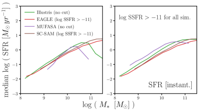
In the left panel of Figure A.1 we reproduce the SFS comparison of Somerville & Davé (2015) Figure 5 for the simulations in Section 2 using different methods for measuring the SFS. For Illustris and EAGLE, we apply the same methods as the SFSs in Somerville & Davé (2015): the median SFR in a $M_{*}$ bin with no selection cut for Illustris (green) and with a SSFR > $10^{-11}\,\mathrm{yr}^{-1}$ cut for EAGLE (red; Schaye et al., 2015). Mufasa and the current version of SC-SAM did not exist and were not included in Somerville & Davé (2015). Since we are illustrating how inconsistent SFS measurements can result in misleading agreement, for Mufasa and SC-SAM we measure the median SFR with no selection cut and with a SSFR > $10^{-11}\,\mathrm{yr}^{-1}$ cut, respectively. As in Figure 5 of Somerville & Davé (2015), we find good agreement among the SFSs of the simulations.

Instead of measuring the SFSs differently, if we measure the SFS by taking the median SFR after a SSFR > $10^{-11}\,\mathrm{yr}^{-1}$ cut consistently for all the simulations, we find discrepancies in the SFSs on the order of ${\sim}0.5\,\mathrm{dex}$ (right panel of A.1). This illustrates that the agreement found in Somerville & Davé (2015) is driven in large part by the difference in methods used to measure SFSs. Furthermore, the difference between the Illustris and Mufasa SFSs in the two panels illustrate how different SFS fitting methods, even when consistently applied, can increase the difference between SFSs. The difference between the Illustris and Mufasa SFSs is significantly larger in the right panel when the SSFR > $10^{-11}\,\mathrm{yr}^{-1}$ cut is applied and galaxies with SFR below the resolution limit, which make up a larger fraction of the Mufasa galaxies than the Illustris galaxies, are removed by the selection cut. This impact highlights the need for a data-driven method for identifying the SFS that better account for intrinsically different SFR–$M_{*}$ distributions in the simulations. Therefore, Figure A.1 highlights the impact of hard selection cuts and the importance of using a consistent data-driven methodology for measuring the SFS.

Appendix B Identifying the SFS using Gaussian Mixture Models

In order to derive the best-fit GMM used for identifying the SFS in each $M_{*}$ bin, we compare GMM fits with $k\leq 3$ components using their BICs (Section 3). In Figures B.1 and B.2, we illustrate this comparison among the GMMs with $k=1,2,$ and $3$ (blue, orange, and green) components fit to the instantaneous SSFR distributions, $P(\log\,\mathrm{SSFR})$, of the Illustris, EAGLE, Mufasa, and SC-SAM (top to bottom panels) centrals in three stellar mass bins: $9.2<\log\,M_{*}<9.4$, $9.8<\log\,M_{*}<10$, and $10.6<\log\,M_{*}<10.8$ (left to right). The SSFR distributions in Figures B.1 and B.2 are derived using instantaneous and $100\,\mathrm{Myr}$ SFRs respectively. Galaxies with unmeasurably low SFR are represented at the edge of the SSFR distributions with $\log\,\mathrm{SSFR}=-13.5$. In each panel, we also present the BICs and plot every component of the GMM fits (dashed) in their respective colors. These figures illustrate the advantages of the data-driven GMM based fitting and BIC based model selection used in our SFS fitting.

Figure B.1: GMMs with $k=1,2,$ and $3$ (blue, orange, and green) components fit to the instantaneous SSFR distributions, $P(\log\,\mathrm{SSFR})$, of the Illustris, EAGLE, Mufasa, and SC-SAM (top to bottom panels) centrals in three stellar mass bins: $[9.2,9.4]$, $[9.8,10.]$, and $[10.6,10.8]$ (left to right). We represent galaxies with unmeasurably low SFR in $P(\log\,\mathrm{SSFR})$s with $\log\,\mathrm{SSFR}=-13.5$. For every GMM fit, we plot each component in dash lines and list their BICs in the same color. In our SFS fitting, we select the GMM with the lowest BIC as the best-fit. This provides a data-driven way of accurately fitting the SSFR distribution while avoiding overfitting.

Figure B.2: Same as Figure B.1 but for the $100\,\mathrm{Myr}$ SSFR distributions.

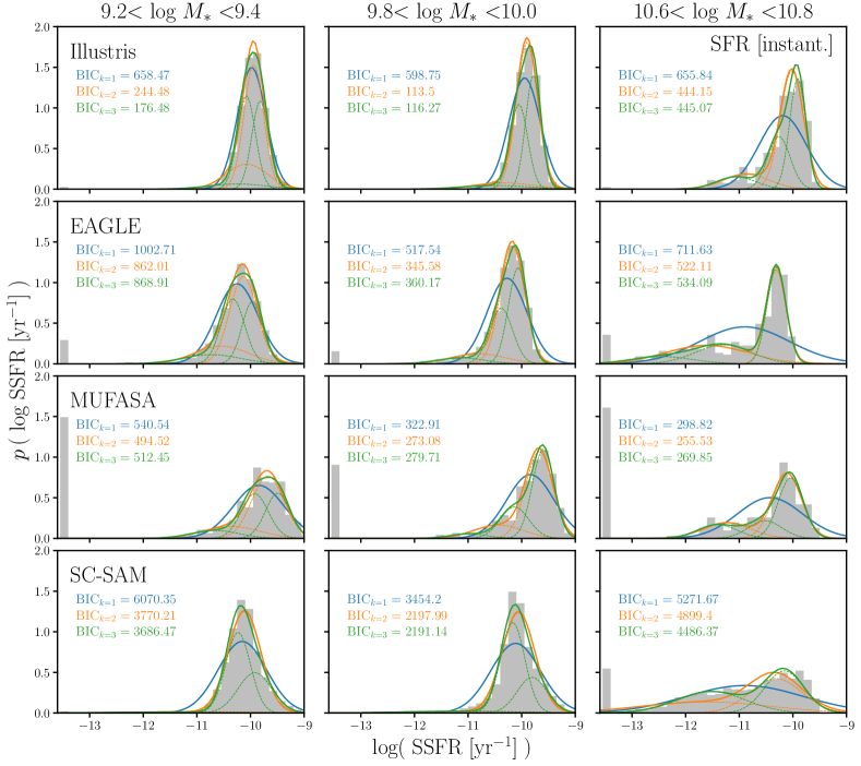
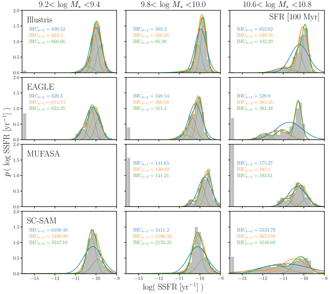
For instance, in most of the highest $M_{*}$ bin (right panels in both figures) the $k=1$ GMM fits do not reflect the clearly bimodal SSFR distributions. In these cases, the $\mathrm{BIC}_{k=1}$ is significantly larger than $\mathrm{BIC}_{k=2}$ and $\mathrm{BIC}_{k=3}$, so our BIC based model selection favors GMMs with more than one component. In fact, GMMs with more components are more flexible and generally can better fit the underlying distribution. However as the EAGLE and Mufasa $9.8<\log\,M_{*}<10$ bins of the figures illustrate, our BIC based model selection does not always favor the higher $k$ GMM fits. Although the $k=3$ GMMs have the lowest $\chi^{2}$ in these panels, because of the penalty term for the number of model parameters, our BIC criteria favors the $k=2$ GMMs. According to the BICs, the $k=3$ GMMs in these panels overfit the SSFR distributions.

From the best-fit GMMs, we identify the SFS components iteratively starting from the lowest $M_{*}$ bin as described in Section 3.1. We consider other components, depending on their mean, as intermediate or high SF components in Section 4.2. The SC-SAM in particular has high SF components at $M_{*}\lesssim 10^{10}M_{\sun}$ (bottom left and center panels of Figures B.1 and B.2). In these cases, the SSFR distribution is not well described by a single log-normal distribution. Instead the distribution is asymmetric with a heavier tail on the more star-forming end of the distribution. An extra component to account for the heavier tail improves the fit more than the penalty term, giving us the high SF components.

Appendix C SFR Resolution Effects in Hydrodynamic Simulations

In our analysis, we consistently derive SFRs for all of the simulated galaxies on two timescales: instantaneous and averaged over $100\,\mathrm{Myr}$ (Section 2). For the hydrodynamic simulations, SFR averaged over $100\,\mathrm{Myr}$ is derived using the formation times of the star particles in the simulation, which means that the mass and temporal resolutions of the simulations impact the $100\,\mathrm{Myr}$ SFR. In Illustris, EAGLE, and Mufasa, their $100\,\mathrm{Myr}$ SFRs have resolutions of $\Delta_{\mathrm{SFR}}=0.0126$, $0.018$, and $0.182\,M_{\sun}\mathrm{yr}^{-1}$, corresponding to baryon particle masses of $1.26\times 10^{6}\ M_{\sun}$, $1.8\times 10^{6}\ M_{\sun}$, and $1.82\times 10^{7}\ M_{\sun}$, respectively. For SFR averaged over $10\,\mathrm{Myr}$, the $\Delta_{\mathrm{SFR}}$s would be 10 times larger. Therefore, we instead use instantaneous SFRs to measure star formation on the shortest timescale.

Figure C.1: The impact of SFR resolution on the SSFR distribution, $P(\log\,\mathrm{SSFR})$, in two stellar mass bins of the hydrodynamic simulations: Illustris (left), EAGLE (center), and Mufasa (right). We plot the $P(\mathrm{SSFR})$ distributions using the $100\,\mathrm{Myr}$ SFRs with resolution effects in black. These exclude galaxies with unmeasurably low SFRs. In orange, we plot the $P(\log\,\mathrm{SSFR})$ distributions where the SFRs of the galaxies are sampled uniformly within the SFR resolution range ($[\mathrm{SFR}_{i},\mathrm{SFR}_{i}+\Delta_{\mathrm{SFR}}]$). The uncertainties for the orange $P(\mathrm{SSFR})$s are estimated from re-sampling the SFR of each galaxy based on the SFR resolution. At low stellar masses (top) the SFR resolution significantly impacts the star-forming end of $P(\mathrm{SSFR})$s. At higher stellar masses, although the SFR resolution impacts the $P(\mathrm{SSFR})$s, the effect is limited to below $\log\,\mathrm{SSFR}<-11$.

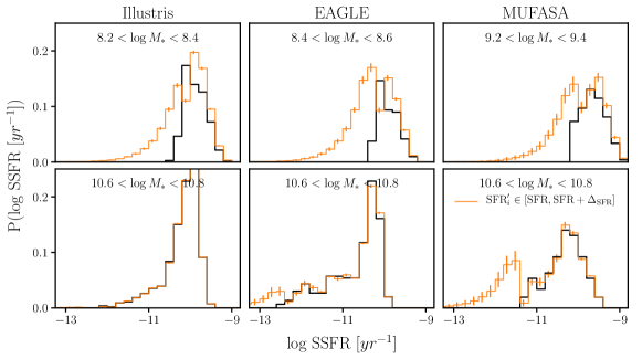
For galaxies with high $100\,\mathrm{Myr}$ SFR, the resolution $\Delta_{\mathrm{SFR}}$ is relatively small compared to their SFRs and therefore it does not have a significant impact. However for low SFR galaxies, the resolution effect is more significant. At the lowest SFR end, galaxies that, without the resolution effect, would have SFR ranging $0<\mathrm{SFR}<\Delta_{\mathrm{SFR}}$, may have unmeasurably low SFR ($\mathrm{SFR}{=}0$) with the resolution effect. These galaxies are thereby not included in the $\mathrm{SFR}$–$M_{*}$ plane or when we identify the SFS. In Figure C.1, we present the impact of excluding these galaxies and the overall resolution effect on the $P(\log\,\mathrm{SSFR})$ distributions of the hydrodynamic simulations in two stellar mass bins. In black, we plot the $P(\log\,\mathrm{SSFR})$ distributions using the $100\,\mathrm{Myr}$ SFRs with resolution effects (excluding galaxies with unmeasurably low SFR). In orange, we plot the $P(\log\,\mathrm{SSFR})$ distributions of all galaxies where $\mathrm{SFR}^{\prime}_{i}$ of each galaxy sampled uniformly within the SFR resolution range, $[\mathrm{SFR}_{i},\mathrm{SFR}_{i}+\Delta_{\mathrm{SFR}}]$. Uncertainties for the orange $P(\log\,\mathrm{SSFR})$s are derived from repeating this SFR sampling $100$ times. For the low $M_{*}$ bins (top), the SFR resolution affects the $P(\log\,\mathrm{SSFR})$s well above $\log\,\mathrm{SSFR}{=}{-}11.0$ on the star-forming end of the distribution. Meanwhile, the impact at higher $M_{*}$ (bottom), is limited to the low SSFR end.

Figure C.2: The resolution effect of $100\,\mathrm{Myr}$ SFRs in the hydrodynamic simulations (Illustris, EAGLE, and Mufasa) impact the identified SFSs at low stellar masses. In black we plot the best-fit SFS with the resolution effects. In orange we plot the best-fit SFS where the SFR for each galaxy is sampled uniformly within the resolution range: $\mathrm{SFR}_{i}^{\prime}\in[\mathrm{SFR}_{i},\mathrm{SFR}_{i}+\Delta_{\mathrm{SFR}}]$). Based on the discrepancy between the fits, we determine stellar mass limits above which the SFR resolution does not significantly impact ($<0.2\,\mathrm{dex}$) the identified SFS. For Illustris, EAGLE, and Mufasa this corresponds to $\log M_{\mathrm{lim}}=8.4,8.4$, and $9.2$, as shown in the gray shaded region.

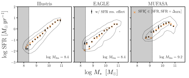
In order to better quantify the impact of the SFR resolution effect on our SFS fitting, in Figure C.2 we compare the SFS fits using $100\,\mathrm{Myr}$ SFRs with resolution effects (black) to the SFS fits using $100\,\mathrm{Myr}$ SFRs sampled uniformly within the SFR resolution range (orange; $\mathrm{SFR}_{i}^{\prime}\in[\mathrm{SFR}_{i},\mathrm{SFR}_{i}+\Delta_{\mathrm{SFR}}]$). The uncertainties of our SFS fits in black are calculated using bootstrap resampling (Section 3). In agreement with Figure C.1, we find that the SFR resolution significantly impacts the identified SFS at low $M_{*}$. Moreover, using the comparison of Figure C.2, we determine the stellar mass limit above which the SFR resolution does not significantly impact the identified SFS — i.e. the shift in best-fit SFS is below $0.2\,\mathrm{dex}$. For Illustris, EAGLE, and Mufasa we determine $\log M_{\mathrm{lim}}=8.4,8.4$, and $9.2$, respectively. For EAGLE, where we have a higher resolution box ($8\times$ higher baryon mass resolution) available, we further confirm that the SFS is not significantly impacted above $\log M_{\mathrm{lim}}$.

Figure C.3: Fractional contributions, $\pi_{i}$, of the best-fit GMM components from our method for the hydrodynamic simulations (Illustris, EAGLE, and Mufasa) where we uniformly sample the $100\,\mathrm{Myr}$ SFRs within the SFR resolution range — $\mathrm{SFR}_{i}^{\prime}\in[\mathrm{SFR}_{i},\mathrm{SFR}_{i}+\Delta_{\mathrm{SFR}}]$. Compared to Figure 9, we find SFR resolution has no significant impact on the qualitative results in Section 4.2.

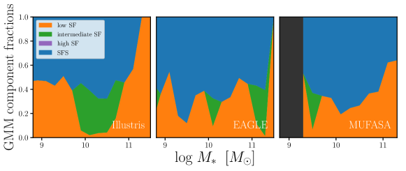
In addition to its effect on the SFS fits, we also examine the impact of SFR resolution on our results regarding the non-SFS components of our GMM fitting (Figure 9). In Figure C.3 we present the fraction contributions ($\pi_{i}$) of the best-fit components for the Illustris, EAGLE, and Mufasa simulations, where we uniformly sample the SFRs within the SFR resolution range (same as above). Besides no longer having a component of galaxies with unmeasurably low SFRs due to the SFR sampling, we find no significant change from the $\pi_{i}$ of Figure 9 and, thus, the results of Section 4.2.

References

- Abazajian et al. (2009) Abazajian, K. N., Adelman-McCarthy, J. K., Agüeros, M. A., et al. 2009, The Astrophysical Journal Supplement Series, 182, 543, doi: 10.1088/0067-0049/182/2/543
- Abramson et al. (2016) Abramson, L. E., Gladders, M. D., Dressler, A., et al. 2016, The Astrophysical Journal, 832, 7, doi: 10.3847/0004-637X/832/1/7
- Aihara et al. (2011) Aihara, H., Allende Prieto, C., An, D., et al. 2011, The Astrophysical Journal Supplement Series, 193, 29, doi: 10.1088/0067-0049/193/2/29
- Arthur & Vassilvitskii (2007) Arthur, D., & Vassilvitskii, S. 2007, in Proceedings of the Eighteenth Annual ACM-SIAM Symposium on Discrete Algorithms, SODA ’07 (Philadelphia, PA, USA: Society for Industrial and Applied Mathematics), 1027–1035
- Astropy Collaboration et al. (2013) Astropy Collaboration, Robitaille, T. P., Tollerud, E. J., et al. 2013, 558, A33, doi: 10.1051/0004-6361/201322068
- Baldry et al. (2006) Baldry, I. K., Balogh, M. L., Bower, R. G., et al. 2006, Monthly Notices of the Royal Astronomical Society, 373, 469, doi: 10.1111/j.1365-2966.2006.11081.x
- Balogh et al. (1998) Balogh, M. L., Schade, D., Morris, S. L., et al. 1998, The Astrophysical Journal Letters, 504, L75, doi: 10.1086/311576
- Behroozi et al. (2013a) Behroozi, P. S., Wechsler, R. H., & Conroy, C. 2013a, The Astrophysical Journal, 770, 57, doi: 10.1088/0004-637X/770/1/57
- Behroozi et al. (2013b) Behroozi, P. S., Wechsler, R. H., & Wu, H.-Y. 2013b, The Astrophysical Journal, 762, 109, doi: 10.1088/0004-637X/762/2/109
- Bigiel et al. (2008) Bigiel, F., Leroy, A., Walter, F., et al. 2008, The Astronomical Journal, 136, 2846, doi: 10.1088/0004-6256/136/6/2846
- Bisigello et al. (2018) Bisigello, L., Caputi, K. I., Grogin, N., & Koekemoer, A. 2018, Astronomy and Astrophysics, 609, A82, doi: 10.1051/0004-6361/201731399
- Blanton (2006) Blanton, M. R. 2006, The Astrophysical Journal, 648, 268, doi: 10.1086/505628
- Blanton et al. (2011) Blanton, M. R., Kazin, E., Muna, D., Weaver, B. A., & Price-Whelan, A. 2011, The Astronomical Journal, 142, 31, doi: 10.1088/0004-6256/142/1/31
- Blanton & Moustakas (2009) Blanton, M. R., & Moustakas, J. 2009, Annual Review of Astronomy and Astrophysics, 47, 159, doi: 10.1146/annurev-astro-082708-101734
- Blanton & Roweis (2007) Blanton, M. R., & Roweis, S. 2007, The Astronomical Journal, 133, 734, doi: 10.1086/510127
- Blanton et al. (2003) Blanton, M. R., Hogg, D. W., Bahcall, N. A., et al. 2003, The Astrophysical Journal, 594, 186, doi: 10.1086/375528
- Blanton et al. (2005) Blanton, M. R., Schlegel, D. J., Strauss, M. A., et al. 2005, The Astronomical Journal, 129, 2562, doi: 10.1086/429803
- Bluck et al. (2016) Bluck, A. F. L., Mendel, J. T., Ellison, S. L., et al. 2016, Monthly Notices of the Royal Astronomical Society, 462, 2559, doi: 10.1093/mnras/stw1665
- Borch et al. (2006) Borch, A., Meisenheimer, K., Bell, E. F., et al. 2006, Astronomy and Astrophysics, 453, 869, doi: 10.1051/0004-6361:20054376
- Bovy et al. (2011) Bovy, J., Hogg, D. W., & Roweis, S. T. 2011, The Annals of Applied Statistics, 5, 1657, doi: 10.1214/10-AOAS439
- Brennan et al. (2015) Brennan, R., Pandya, V., Somerville, R. S., et al. 2015, Monthly Notices of the Royal Astronomical Society, 451, 2933, doi: 10.1093/mnras/stv1007
- Brennan et al. (2017) —. 2017, Monthly Notices of the Royal Astronomical Society, 465, 619, doi: 10.1093/mnras/stw2690
- Brinchmann et al. (2004) Brinchmann, J., Charlot, S., White, S. D. M., et al. 2004, Monthly Notices of the Royal Astronomical Society, 351, 1151, doi: 10.1111/j.1365-2966.2004.07881.x
- Broderick et al. (2011) Broderick, A. E., Fish, V. L., Doeleman, S. S., & Loeb, A. 2011, The Astrophysical Journal, 735, 110, doi: 10.1088/0004-637X/735/2/110
- Bruzual A. & Charlot (1993) Bruzual A., G., & Charlot, S. 1993, The Astrophysical Journal, 405, 538, doi: 10.1086/172385
- Bundy et al. (2006) Bundy, K., Ellis, R. S., Conselice, C. J., et al. 2006, The Astrophysical Journal, 651, 120, doi: 10.1086/507456
- Chabrier (2003) Chabrier, G. 2003, Publications of the Astronomical Society of the Pacific, 115, 763, doi: 10.1086/376392
- Charlot & Fall (2000) Charlot, S., & Fall, S. M. 2000, The Astrophysical Journal, 539, 718, doi: 10.1086/309250
- Collaboration et al. (2018) Collaboration, T. A., Price-Whelan, A. M., Sipőcz, B. M., et al. 2018, The Astronomical Journal, 156, 123, doi: 10.3847/1538-3881/aabc4f
- Crain et al. (2015) Crain, R. A., Schaye, J., Bower, R. G., et al. 2015, Monthly Notices of the Royal Astronomical Society, 450, 1937, doi: 10.1093/mnras/stv725
- Daddi et al. (2007) Daddi, E., Dickinson, M., Morrison, G., et al. 2007, The Astrophysical Journal, 670, 156, doi: 10.1086/521818
- Dalla Vecchia & Schaye (2012) Dalla Vecchia, C., & Schaye, J. 2012, Monthly Notices of the Royal Astronomical Society, 426, 140, doi: 10.1111/j.1365-2966.2012.21704.x
- Davé et al. (2017a) Davé, R., Rafieferantsoa, M. H., & Thompson, R. J. 2017a, arXiv:1704.01135 [astro-ph]. https://arxiv.org/abs/1704.01135
- Davé et al. (2017b) Davé, R., Rafieferantsoa, M. H., Thompson, R. J., & Hopkins, P. F. 2017b, Monthly Notices of the Royal Astronomical Society, 467, 115, doi: 10.1093/mnras/stx108
- Davé et al. (2016) Davé, R., Thompson, R., & Hopkins, P. F. 2016, Monthly Notices of the Royal Astronomical Society, 462, 3265, doi: 10.1093/mnras/stw1862
- Davis et al. (1985) Davis, M., Efstathiou, G., Frenk, C. S., & White, S. D. M. 1985, The Astrophysical Journal, 292, 371, doi: 10.1086/163168
- Dempster et al. (1977) Dempster, A. P., Laird, N. M., & Rubin, D. B. 1977, Journal of the Royal Statistical Society. Series B (Methodological), 39, 1
- Efron (1979) Efron, B. 1979, The Annals of Statistics, 7, 1, doi: 10.1214/aos/1176344552
- Feldmann (2017) Feldmann, R. 2017, Monthly Notices of the Royal Astronomical Society, 470, L59, doi: 10.1093/mnrasl/slx073
- Ferland (1996) Ferland, G. J. 1996, Hazy, A Brief Introduction to Cloudy 90
- Fraley & Raftery (1998) Fraley, C., & Raftery, A. E. 1998, The Computer Journal, 41, 578, doi: 10.1093/comjnl/41.8.578
- Furlong et al. (2015) Furlong, M., Bower, R. G., Theuns, T., et al. 2015, Monthly Notices of the Royal Astronomical Society, 450, 4486, doi: 10.1093/mnras/stv852
- Gabor & Davé (2015) Gabor, J. M., & Davé, R. 2015, Monthly Notices of the Royal Astronomical Society, 447, 374, doi: 10.1093/mnras/stu2399
- Geha et al. (2012) Geha, M., Blanton, M. R., Yan, R., & Tinker, J. L. 2012, The Astrophysical Journal, 757, 85, doi: 10.1088/0004-637X/757/1/85
- Genel et al. (2014) Genel, S., Vogelsberger, M., Springel, V., et al. 2014, Monthly Notices of the Royal Astronomical Society, 445, 175, doi: 10.1093/mnras/stu1654
- Gill et al. (2005) Gill, S. P. D., Knebe, A., & Gibson, B. K. 2005, Monthly Notices of the Royal Astronomical Society, 356, 1327, doi: 10.1111/j.1365-2966.2004.08562.x
- Gnedin & Kravtsov (2011) Gnedin, N. Y., & Kravtsov, A. V. 2011, The Astrophysical Journal, 728, 88, doi: 10.1088/0004-637X/728/2/88
- Hahn et al. (2017) Hahn, C., Tinker, J. L., & Wetzel, A. R. 2017, The Astrophysical Journal, 841, 6, doi: 10.3847/1538-4357/aa6d6b
- Hahn et al. (2015) Hahn, C., Blanton, M. R., Moustakas, J., et al. 2015, The Astrophysical Journal, 806, 162, doi: 10.1088/0004-637X/806/2/162
- Hao et al. (2009) Hao, J., Koester, B. P., Mckay, T. A., et al. 2009, The Astrophysical Journal, 702, 745, doi: 10.1088/0004-637X/702/1/745
- Hopkins & Beacom (2006) Hopkins, A. M., & Beacom, J. F. 2006, The Astrophysical Journal, 651, 142, doi: 10.1086/506610
- Hopkins (2015) Hopkins, P. F. 2015, Monthly Notices of the Royal Astronomical Society, 450, 53, doi: 10.1093/mnras/stv195
- Hunter (2007) Hunter, J. D. 2007, Computing In Science & Engineering, 9, 90
- Iovino et al. (2010) Iovino, A., Cucciati, O., Scodeggio, M., et al. 2010, Astronomy and Astrophysics, 509, A40, doi: 10.1051/0004-6361/200912558
- Jones et al. (2001) Jones, E., Oliphant, T., Peterson, P., & others. 2001
- Kauffmann et al. (2003) Kauffmann, G., Heckman, T. M., White, S. D. M., et al. 2003, Monthly Notices of the Royal Astronomical Society, 341, 54, doi: 10.1046/j.1365-8711.2003.06292.x
- Kelson (2014) Kelson, D. D. 2014, arXiv:1406.5191 [astro-ph]. https://arxiv.org/abs/1406.5191
- Kennicutt & Evans (2012) Kennicutt, R. C., & Evans, N. J. 2012, Annual Review of Astronomy and Astrophysics, 50, 531, doi: 10.1146/annurev-astro-081811-125610
- Krumholz & Gnedin (2011) Krumholz, M. R., & Gnedin, N. Y. 2011, The Astrophysical Journal, 729, 36, doi: 10.1088/0004-637X/729/1/36
- Lee et al. (2012) Lee, K. J., Guillemot, L., Yue, Y. L., Kramer, M., & Champion, D. J. 2012, Monthly Notices of the Royal Astronomical Society, 424, 2832, doi: 10.1111/j.1365-2966.2012.21413.x
- Lee et al. (2015) Lee, N., Sanders, D. B., Casey, C. M., et al. 2015, The Astrophysical Journal, 801, 80, doi: 10.1088/0004-637X/801/2/80
- Leja et al. (2015) Leja, J., van Dokkum, P. G., Franx, M., & Whitaker, K. E. 2015, 798, 115, doi: 10.1088/0004-637X/798/2/115
- Leroux (1992) Leroux, B. G. 1992, The Annals of Statistics, 20, 1350, doi: 10.1214/aos/1176348772
- Liddle (2007) Liddle, A. R. 2007, Monthly Notices of the Royal Astronomical Society, 377, L74, doi: 10.1111/j.1745-3933.2007.00306.x
- Lloyd (1982) Lloyd, S. 1982, IEEE Transactions on Information Theory, 28, 129, doi: 10.1109/TIT.1982.1056489
- Madau & Dickinson (2014) Madau, P., & Dickinson, M. 2014, Annual Review of Astronomy and Astrophysics, 52, 415, doi: 10.1146/annurev-astro-081811-125615
- Magdis et al. (2012) Magdis, G. E., Daddi, E., Béthermin, M., et al. 2012, The Astrophysical Journal, 760, 6, doi: 10.1088/0004-637X/760/1/6
- Mamon et al. (2004) Mamon, G. A., Sanchis, T., Salvador-Solé, E., & Solanes, J. M. 2004, Astronomy and Astrophysics, 414, 445, doi: 10.1051/0004-6361:20034155
- McAlpine et al. (2016) McAlpine, S., Helly, J. C., Schaller, M., et al. 2016, Astronomy and Computing, 15, 72, doi: 10.1016/j.ascom.2016.02.004
- McLachlan & Peel (2000) McLachlan, G., & Peel, D. 2000, Finite Mixture Models (Wiley-Interscience)
- Mitra et al. (2015) Mitra, S., Davé, R., & Finlator, K. 2015, Monthly Notices of the Royal Astronomical Society, 452, 1184, doi: 10.1093/mnras/stv1387
- Moustakas et al. (2013) Moustakas, J., Coil, A. L., Aird, J., et al. 2013, The Astrophysical Journal, 767, 50, doi: 10.1088/0004-637X/767/1/50
- Muratov et al. (2015) Muratov, A. L., Kereš, D., Faucher-Giguère, C.-A., et al. 2015, Monthly Notices of the Royal Astronomical Society, 454, 2691, doi: 10.1093/mnras/stv2126
- Neal & Hinton (1998) Neal, R. M., & Hinton, G. E. 1998, in Learning in Graphical Models, NATO ASI Series (Springer, Dordrecht), 355–368
- Nelson et al. (2015) Nelson, D., Pillepich, A., Genel, S., et al. 2015, Astronomy and Computing, 13, 12, doi: 10.1016/j.ascom.2015.09.003
- Noeske et al. (2007) Noeske, K. G., Weiner, B. J., Faber, S. M., et al. 2007, The Astrophysical Journal Letters, 660, L43, doi: 10.1086/517926
- Oppenheimer & Davé (2006) Oppenheimer, B. D., & Davé, R. 2006, Monthly Notices of the Royal Astronomical Society, 373, 1265, doi: 10.1111/j.1365-2966.2006.10989.x
- Pandya et al. (2017) Pandya, V., Brennan, R., Somerville, R. S., et al. 2017, Monthly Notices of the Royal Astronomical Society, 472, 2054, doi: 10.1093/mnras/stx2027
- Pedregosa et al. (2011) Pedregosa, F., Varoquaux, G., Gramfort, A., et al. 2011, Journal of machine learning research, 12, 2825
- Peng et al. (2010) Peng, Y.-j., Lilly, S. J., Kovač, K., et al. 2010, The Astrophysical Journal, 721, 193, doi: 10.1088/0004-637X/721/1/193
- Popping et al. (2014) Popping, G., Somerville, R. S., & Trager, S. C. 2014, Monthly Notices of the Royal Astronomical Society, 442, 2398, doi: 10.1093/mnras/stu991
- Porter et al. (2014) Porter, L. A., Somerville, R. S., Primack, J. R., & Johansson, P. H. 2014, Monthly Notices of the Royal Astronomical Society, 444, 942, doi: 10.1093/mnras/stu1434
- Press et al. (1992) Press, W. H., Teukolsky, S. A., Vetterling, W. T., & Flannery, B. P. 1992, Numerical Recipes in C (2Nd Ed.): The Art of Scientific Computing (New York, NY, USA: Cambridge University Press)
- Rodríguez-Puebla et al. (2016) Rodríguez-Puebla, A., Primack, J. R., Behroozi, P., & Faber, S. M. 2016, Monthly Notices of the Royal Astronomical Society, 455, 2592, doi: 10.1093/mnras/stv2513
- Roeder & Wasserman (1997) Roeder, K., & Wasserman, L. 1997, Journal of the American Statistical Association, 92, 894, doi: 10.1080/01621459.1997.10474044
- Salim et al. (2007) Salim, S., Rich, R. M., Charlot, S., et al. 2007, The Astrophysical Journal Supplement Series, 173, 267, doi: 10.1086/519218
- Schaller et al. (2015) Schaller, M., Dalla Vecchia, C., Schaye, J., et al. 2015, 454, 2277, doi: 10.1093/mnras/stv2169
- Schaye et al. (2015) Schaye, J., Crain, R. A., Bower, R. G., et al. 2015, Monthly Notices of the Royal Astronomical Society, 446, 521, doi: 10.1093/mnras/stu2058
- Schreiber et al. (2015) Schreiber, C., Pannella, M., Elbaz, D., et al. 2015, Astronomy and Astrophysics, 575, A74, doi: 10.1051/0004-6361/201425017
- Schwarz (1978) Schwarz, G. 1978, The Annals of Statistics, 6, 461, doi: 10.1214/aos/1176344136
- Sijacki et al. (2007) Sijacki, D., Springel, V., Di Matteo, T., & Hernquist, L. 2007, Monthly Notices of the Royal Astronomical Society, 380, 877, doi: 10.1111/j.1365-2966.2007.12153.x
- Somerville & Davé (2015) Somerville, R. S., & Davé, R. 2015, Annual Review of Astronomy and Astrophysics, 53, 51, doi: 10.1146/annurev-astro-082812-140951
- Somerville et al. (2012) Somerville, R. S., Gilmore, R. C., Primack, J. R., & Domínguez, A. 2012, Monthly Notices of the Royal Astronomical Society, 423, 1992, doi: 10.1111/j.1365-2966.2012.20490.x
- Somerville et al. (2008a) Somerville, R. S., Hopkins, P. F., Cox, T. J., Robertson, B. E., & Hernquist, L. 2008a, Monthly Notices of the Royal Astronomical Society, 391, 481, doi: 10.1111/j.1365-2966.2008.13805.x
- Somerville et al. (2015) Somerville, R. S., Popping, G., & Trager, S. C. 2015, Monthly Notices of the Royal Astronomical Society, 453, 4337, doi: 10.1093/mnras/stv1877
- Somerville & Primack (1999) Somerville, R. S., & Primack, J. R. 1999, Monthly Notices of the Royal Astronomical Society, 310, 1087, doi: 10.1046/j.1365-8711.1999.03032.x
- Somerville et al. (2001) Somerville, R. S., Primack, J. R., & Faber, S. M. 2001, Monthly Notices of the Royal Astronomical Society, 320, 504, doi: 10.1046/j.1365-8711.2001.03975.x
- Somerville et al. (2008b) Somerville, R. S., Barden, M., Rix, H.-W., et al. 2008b, The Astrophysical Journal, 672, 776, doi: 10.1086/523661
- Sparre et al. (2017) Sparre, M., Hayward, C. C., Feldmann, R., et al. 2017, Monthly Notices of the Royal Astronomical Society, 466, 88, doi: 10.1093/mnras/stw3011
- Sparre et al. (2015) Sparre, M., Hayward, C. C., Springel, V., et al. 2015, Monthly Notices of the Royal Astronomical Society, 447, 3548, doi: 10.1093/mnras/stu2713
- Speagle et al. (2014) Speagle, J. S., Steinhardt, C. L., Capak, P. L., & Silverman, J. D. 2014, The Astrophysical Journal Supplement Series, 214, 15, doi: 10.1088/0067-0049/214/2/15
- Springel (2005) Springel, V. 2005, Monthly Notices of the Royal Astronomical Society, 364, 1105, doi: 10.1111/j.1365-2966.2005.09655.x
- Springel (2010) —. 2010, 401, 791, doi: 10.1111/j.1365-2966.2009.15715.x
- Springel & Hernquist (2003) Springel, V., & Hernquist, L. 2003, Monthly Notices of the Royal Astronomical Society, 339, 289, doi: 10.1046/j.1365-8711.2003.06206.x
- Springel et al. (2001) Springel, V., White, S. D. M., Tormen, G., & Kauffmann, G. 2001, Monthly Notices of the Royal Astronomical Society, 328, 726, doi: 10.1046/j.1365-8711.2001.04912.x
- Steele & Raftery (2010) Steele, R. J., & Raftery, A. E. 2010
- Taylor et al. (2009) Taylor, E. N., Franx, M., van Dokkum, P. G., et al. 2009, The Astrophysical Journal, 694, 1171, doi: 10.1088/0004-637X/694/2/1171
- Taylor et al. (2015) Taylor, E. N., Hopkins, A. M., Baldry, I. K., et al. 2015, Monthly Notices of the Royal Astronomical Society, 446, 2144, doi: 10.1093/mnras/stu1900
- Terrazas et al. (2017) Terrazas, B. A., Bell, E. F., Woo, J., & Henriques, B. M. B. 2017, The Astrophysical Journal, 844, 170, doi: 10.3847/1538-4357/aa7d07
- Tinker et al. (2011) Tinker, J., Wetzel, A., & Conroy, C. 2011, ArXiv e-prints, 1107, arXiv:1107.5046
- Torrey et al. (2014) Torrey, P., Vogelsberger, M., Genel, S., et al. 2014, Monthly Notices of the Royal Astronomical Society, 438, 1985, doi: 10.1093/mnras/stt2295
- Trayford et al. (2015) Trayford, J. W., Theuns, T., Bower, R. G., et al. 2015, Monthly Notices of the Royal Astronomical Society, 452, 2879, doi: 10.1093/mnras/stv1461
- Trayford et al. (2017) Trayford, J. W., Camps, P., Theuns, T., et al. 2017, Monthly Notices of the Royal Astronomical Society, 470, 771, doi: 10.1093/mnras/stx1051
- Vakili & Hahn (2016) Vakili, M., & Hahn, C. H. 2016, arXiv:1610.01991 [astro-ph]. https://arxiv.org/abs/1610.01991
- Van Der Walt et al. (2011) Van Der Walt, S., Colbert, S. C., & Varoquaux, G. 2011, ArXiv e-prints, arXiv:1102.1523. https://arxiv.org/abs/1102.1523
- Vanderplas et al. (2012) Vanderplas, J., Connolly, A., Ivezi’c, Z., & Gray, A. 2012, in Conference on Intelligent Data Understanding (CIDU), 47–54
- Vogelsberger et al. (2013) Vogelsberger, M., Genel, S., Sijacki, D., et al. 2013, Monthly Notices of the Royal Astronomical Society, 436, 3031, doi: 10.1093/mnras/stt1789
- Vogelsberger et al. (2014) Vogelsberger, M., Genel, S., Springel, V., et al. 2014, Monthly Notices of the Royal Astronomical Society, 444, 1518, doi: 10.1093/mnras/stu1536
- Wang et al. (2009) Wang, H., Mo, H. J., & Jing, Y. P. 2009, Monthly Notices of the Royal Astronomical Society, 396, 2249, doi: 10.1111/j.1365-2966.2009.14884.x
- Wang et al. (2013) Wang, L., Farrah, D., Oliver, S. J., et al. 2013, Monthly Notices of the Royal Astronomical Society, 431, 648, doi: 10.1093/mnras/stt190
- Wang et al. (2018) Wang, L., Norberg, P., Brough, S., et al. 2018, arXiv:1802.08456 [astro-ph]. https://arxiv.org/abs/1802.08456
- Wetzel et al. (2012) Wetzel, A. R., Tinker, J. L., & Conroy, C. 2012, Monthly Notices of the Royal Astronomical Society, 424, 232, doi: 10.1111/j.1365-2966.2012.21188.x
- Wetzel et al. (2013) Wetzel, A. R., Tinker, J. L., Conroy, C., & van den Bosch, F. C. 2013, Monthly Notices of the Royal Astronomical Society, 432, 336, doi: 10.1093/mnras/stt469
- Wetzel et al. (2014) —. 2014, Monthly Notices of the Royal Astronomical Society, 439, 2687, doi: 10.1093/mnras/stu122
- Whitaker et al. (2012) Whitaker, K. E., van Dokkum, P. G., Brammer, G., & Franx, M. 2012, The Astrophysical Journal Letters, 754, L29, doi: 10.1088/2041-8205/754/2/L29
- Yan (2011) Yan, R. 2011, The Astronomical Journal, 142, 153, doi: 10.1088/0004-6256/142/5/153
- Yan & Blanton (2012) Yan, R., & Blanton, M. R. 2012, The Astrophysical Journal, 747, 61, doi: 10.1088/0004-637X/747/1/61
- York et al. (2000) York, D. G., Adelman, J., Anderson, Jr., J. E., et al. 2000, The Astronomical Journal, 120, 1579, doi: 10.1086/301513