Tunneling into a finite Luttinger liquid coupled to noisy capacitive leads

Abstract

Tunneling spectroscopy of one-dimensional interacting wires can be profoundly sensitive to the boundary conditions of the wire. Here, we analyze the tunneling spectroscopy of a wire coupled to capacitive metallic leads. Strikingly, with increasing many-body interactions in the wire, the impact of the boundary noise becomes more prominent. This interplay allows for a smooth crossover from standard 1D tunneling signatures into a regime where the tunneling is dominated by the fluctuations at the leads. This regime is characterized by an elevated zero-bias tunneling alongside a universal power-law decay at high energies. Furthermore, local tunneling measurements in this regime show a unique spatial-dependence that marks the formation of plasmonic standing waves in the wire. Our result offers a tunable method by which to control the boundary effects and measure the interaction strength (Luttinger parameter) within the wire.

Advances in control and design of mesoscopic systems have made it possible to realize a variety of ultra-small electronic tunnel-junctions Ingold and Nazarov (1992); Ihn (2004). In such junctions, many-body interactions and coherent effects compete with the charge fluctuations and impedance of the environment to profoundly impact the resulting tunneling characteristics; the tunneling inside the junction excites the electromagnetic modes of an external circuit making it extremely sensitive to the circuit’s impedance Ingold and Nazarov (1992); Ihn (2004); Ingold and Nazarov (2005). This competition alters the tunneling density of states (TDOS) of the various device constituents, with a wide variety of such effects seen in, e.g., normal-metal tunnel-junctions Josephson (1971), Josephon junctions Josephson (1962) and transmission lines Chakravarty and Schmid (1986). Particular examples of such effects include, among others, the Coulomb blockade Kouwenhoven et al. (2001), the Kondo effect Goldhaber-Gordon et al. (1998); Kouwenhoven and Glazman (2001); Rössler et al. (2015) and Andreev bound modes Andreev (1964); van Woerkom et al. (2017); Suominen et al. (2017); Das et al. (2012).

Tunnel-junctions involving one-dimensional (1D) quantum wires are especially intriguing, since many-body interactions fundamentally alter the emergent many-body physics compared with conventional Fermi-liquid metals. Interacting wires are better described using Tomonaga-Luttinger liquid (TLL) theory Tomonaga (1950); Luttinger (1963); Haldane (1981): the low-energy elementary excitations in 1D appear as collective bosonic plasmon modes — in stark contrast to the constitutive fermionic electrons. Consequently, 1D systems show exotic phenomena, such as charge fractionalization of injected electrons Safi and Schulz (1995); Rosenow et al. (2016), spin-charge separation Auslaender and et al. (2005); Jompol and et al. (2009), and zero-bias anomalies (ZBA) Kane and Fisher (1992a); Matveev and Glazman (1993); Mishchenko et al. (2001); Gutman et al. (2008), all of which uniquely interplay with disorder Apel and Rice (1982); Giamarchi and Schulz (1988), quasi-disorder Vidal et al. (2000), and dissipation Altland et al. (2012, 2015). Such 1D effects are ubiquitous and have been observed in a wide variety of systems, including nanotubes Bockrath and et al. (1999); Yao and et al. (1999), GaAs wires Auslaender and et al. (2005); Jompol and et al. (2009), quantum Hall edges Wen (1990); Chang (2003); Ji et al. (2003), as well as, chains of spins or atoms Blumenstein and et al. (2011); Krinner et al. (2015).

More recently, significant progress was made in the description of realistic finite-sized 1D wires with boundary conditions both in- and out-equilibrium Giamarchi (2003); Levkivskyi (2012); Gutman et al. (2008, 2009, 2010). These can generally be grouped into wires (i) with open boundaries Eggert et al. (1996); Schneider et al. (2008); Nazarov et al. (1997), (ii) connected to ohmic contacts Slobodeniuk et al. (2013), or (iii) coupled to inherently out-of-equilibrium charge distributions Gutman et al. (2008, 2009). Interestingly, despite the fact that the many-body interactions profoundly alter the emergent quasiparticle excitations in the wire relative to the electronic boundaries, the wire–boundary interplay cannot be revealed in DC-transport measurements due to the suppression of electron backscattering in clean wires Kane and Fisher (1992b); Giamarchi (2003); Matveev et al. (2010). In contrast, a tunnel-junction between a superconducting or metallic scanning tunneling microscope (STM) and the wire is ideally suited to sense these effects, since it gives access to the wire’s energy distribution function Pothier et al. (1997); Anthore et al. (2003), or to the (local) TDOS Luther and Peschel (1974) of the wire, respectively. The latter commonly displays power-law scaling dependent on the extent of many-body interactions in the system Giamarchi (2003); Fisher and Glazman (1997) – quantified by the Luttinger parameter $K$ – and is strongly impacted by the boundaries, i.e. impedance of the environment Ingold and Nazarov (2005).

In this work, we study the impact of noisy capacitive metallic leads on tunneling into an interacting quantum wire. The capacitance in the leads imposes a finite response time in the wire, suppressing its fast high-energy excitations. Surprisingly, with increasing many-body interactions, the impact of the boundary noise on the wire is enhanced, and its TDOS displays this interplay by entering a regime where it is dominated by the classical impedance of the capacitive reservoirs: at low energies, the finite length of the wire cuts off the expected 1D tunneling zero-bias anomaly Nazarov et al. (1997); Fisher and Glazman (1997), and a zero-bias tunneling peak appears instead as a function of the environment capacitance; at high energies, the characteristic power-law growth is replaced by a universal $\omega^{-3}$ decay Ingold and Nazarov (2005). Interestingly, this wire–environment competition introduces a unique spatial dependence to the TDOS, thus offering an external handle by which to control the correlations in the wire, such that its Luttinger parameter can be tunably detected.

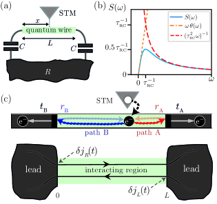
Figure 1: (a) A 1D metallic quantum wire of length $L$ is connected to metallic leads, depicted as an outer circuit that is characterized by an ohmic resistance $R$ and the capacitance $C$. The leads act as electron reservoirs with well-defined Fermi-Dirac distributions. The tunneling density of states [Eq. (1)] at position $x$ along the wire is probed by a nearby scanning tunneling microscope (STM). (b) The zero temperature power spectral-density $S(\omega)$ of the RC-circuit’s noise [Eq. (3)] (blue solid line) and two asymptotic limits: (i) $\omega\,\tau_{\textrm{\tiny RC}}\ll 1$ (orange dot-dashed line) corresponding to the behavior of ideal ohmic leads Lifshitz and Pitaevskii (1980) and (ii) $\omega\,\tau_{\textrm{\tiny RC}}\gg 1$ (red dashed line) where high-energy fluctuations are damped by the circuit’s capacitance. (c) (Top) An electron from the STM induces 1D plasmonic excitations, for which the finite wire acts as an effective Fabry-Pérot interferometer with reflection (transmission) coefficients $r_{{\rm A,B}}$ ($t_{{\rm A,B}}$). (Bottom) A schematic view of the wire as left/right-propagating modes connected to two identical leads, that impart current fluctuations $\delta j_{L/R}(t)$ onto the wire [Eq. (3)].

We consider a finite 1D wire coupled to metallic leads, depicted as an outer circuit that is characterized by an ohmic resistance $R$ and the capacitance $C$, and probed by a nearby STM, see Fig 1(a). The STM signal measures the local TDOS at position $x$ along the wire Bruus and Flensberg (2004)

$$\nu(x,\omega)\!=i\!\!\int\differential t\,e^{i\omega t}\,\left(G^{>}(x,t)-G^{<}(x,t)\right),$$ (1)

where $\omega$ is the electron’s energy, and $G^{<}(x,t)$ and $G^{>}(x,t)$ are the lesser and greater Green’s functions, respectively. We work in natural units, where $\hbar,e=1$. In equilibrium, $G^{<}(x,t)=-G^{>}(x,-t)$ Bruus and Flensberg (2004) and it suffices to analyze $G^{<}(x,t)=i\,\expectationvalue{\psi^{\dagger}(x,t)\psi(x,0)}$, where we wrote its definition using the electronic field-operator $\psi(x,t)$, and the average is taken with respect to the equilibrium ground state.

In $1$D, interacting electrons form a TLL with collective wave-like plasmonic excitations Tomonaga (1950); Luttinger (1963); Haldane (1981); Giamarchi (2003); von Delft and Schoeller (1998). An electron injected from the STM into the wire excites plasmonic modes that propagate away such that the probability amplitude for the excitation to tunnel back into the STM decreases faster than in a non-interacting system. This decay manifests as a power-law in the Green’s function von Delft and Schoeller (1998); Levkivskyi (2012); Gutman et al. (2010)

$$\lim_{L\to\infty}G^{<}(x,t)=\frac{i\,\Lambda}{2\pi v_{F}}\frac{1}{(1+i\Lambda t)^{\alpha}}\,,$$ (2)

where $L$ is the length of the wire, $\Lambda$ is the bandwidth of the electronic system, $v_{F}$ is the Fermi velocity, and $\alpha=\left(K+K^{-1}\right)/2\geq 1$ is the interaction-dependent power-law exponent for the Luttinger parameter $K$. For non-interacting systems $K=1$, and therefore $\alpha=1$.

In a finite wire, the effects of many-body interactions compete with the noise arising at the boundaries Gutman et al. (2008, 2009); Levkivskyi (2012); Slobodeniuk et al. (2013). The latter is characterized, in our case, by a power spectral-density Machlup (1954); Carmi and Oreg (2012); Shahmoon and Leonhardt (2018)

$$S(\omega) \equiv\expectationvalue{\delta j_{L/R}(\omega)\delta j_{L/R}(-\omega)}=\frac{\omega\cdot(1-f_{FD}(\omega))}{1+\tau_{\textrm{\tiny RC}}^{2}\omega^{2}}\,,$$ (3)

where $\tau_{\textrm{\tiny RC}}=RC$ is the discharge time of the capacitor in the outer circuit, and $f_{FD}(\omega)=(1+\exp[-\omega/k_{B}T])^{-1}$ is the Fermi-Dirac distribution in the left and right leads – assumed here to be identical and uncorrelated. The main difference between (3) and the power spectral-density of ideal ohmic leads is that the RC-circuit acts as an additional low-pass filter Levkivskyi (2012); Lifshitz and Pitaevskii (1980), see Fig. 1(b).

We are interested in how the boundary noise (3) and interaction-induced 1D plasmons manifest in the electronic correlations in the wire, e.g., in $G^{<}(x,t)$. While the noise is characterized by the discharge time $\tau_{\textrm{\tiny RC}}$, we shall see below that the plasmonic waves are characterized by their time-of-flight $\tau$ through the finite wire, cf. Eq. (9). We provide here first a brief overview of our main results: the finite discharge time of the leads imposes two distinct regimes, (i) strong-capacitance regime (see Fig. 2), where the time-of-flight is much shorter than the discharge time, $\tau\ll\tau_{\textrm{\tiny RC}}$, and (ii) the more commonly studied complementary weak-capacitance regime with $\tau\gg\tau_{\textrm{\tiny RC}}$. The latter shows a standard TLL behavior for short times $t\leq\tau$, whereas for long times the finite wire acts as a 0D Fabry-Pérot cavity for the plasmons and free-electron correlations are reobtained (cf. Refs. Nazarov et al. (1997); Ingold and Nazarov (2005)). Case (i) shows a richer behavior: at short times ($t\ll\tau,\tau_{\textrm{\tiny RC}}$), the boundary noise inhibits highly-excited plasmons and consequently suppresses tunneling, whereas at long times ($t\gg\tau,\tau_{\textrm{\tiny RC}}$), both the interactions and noise correlations are averaged-out to yield a similar 0D plasmonic Fabry-Pérot behavior. Interestingly, at intermediate times ($\tau<t<\tau_{\textrm{\tiny RC}}$), a competition between the TLL correlations and the boundary response ensues, showing both Fabry-Pérot oscillations, as well as non-trivial power-laws in the electronic correlations, cf. Eq. (10) and see Fig. 2(a). Furthermore, the power-laws show an unexpected dependence on the STM’s position Note (4) that can be observed through [see Fig. 2(b)]

$$\tilde{g}(x,t)\equiv\frac{G^{<}(x,t)}{G^{<}(L/2,t)}\,.$$ (4)

In Fig. LABEL:main_fig:TDOS(a), we plot the TDOS in the strong-capacitance regime. The spatial dependence can be seen in the intermediate energy regime, see Fig. LABEL:main_fig:TDOS(b). For comparison, in Fig. LABEL:main_fig:TDOS(c) we plot the TDOS for both finite- and infinite-length interacting wires. The relatively flat peak of the TDOS at low energies is a result of the finite-length of the wire that suppresses the ZBA of an infinite TLL [Fig. LABEL:main_fig:TDOS(c)], and is in agreement with the free-electron behavior of the Green’s function at long times, cf. Fig. 2(a) and Refs. Nazarov et al. (1997); sup . At high energies, interaction-induced Fabry-Pérot oscillations appear but there is no interaction-dependent power-law growth as compared with both the finite- and infinite-TLL, where the TDOS grows as $\nu(\omega)/\nu_{0}\propto\omega^{\alpha-1}$, with $\alpha=(K+K^{-1})/2$ and $\nu_{0}=\nu(\omega,\tau_{\textrm{\tiny RC}}=0,K=1)$ the TDOS into a non-interacting metal with zero capacitance. This is a consequence of a linear, interaction-independent growth of the Green’s function at short times, see Fig. 2(a). Hence, the noise of the capacitive leads suppresses the power-law growth and causes the TDOS to drop as $\nu/\nu_{0}\propto\omega^{-3}$, in similitude to high-impedance tunnel-junctions Ingold and Nazarov (1992, 2005).

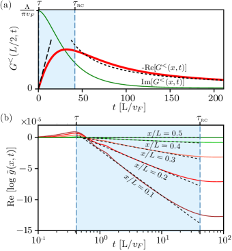
Figure 2: The Green’s function of the wire in the strong-capacitance limit. (a) The imaginary (thin green line) and real (thick red line) part of a lesser Green’s function $G^{<}(L/2,t)$ [Eq. (7)]. The dashed lines show the analytically obtained asymptotic limits for long ($t\gg\tau_{\textrm{\tiny RC}}$) and short ($t\ll\tau_{\textrm{\tiny RC}}$) times. The shaded region (light blue) marks the time interval $\tau<t<\tau_{RC}$ where the interaction-induced correlations in the wire compete with the RC noise. (b) The real part of $\log(\tilde{g}(x,t))$ [Eq. (4)] exhibiting the non-trivial power-law behavior of the Green’s function depending on the position of the STM tip (solid lines). Furthermore, our analytical asymptotic result (dashed lines) [Eq. (11)] agrees with the numerical result (solid lines). In all plots, we use an experimentally realizable interaction parameter $U/v_{F}=15$, see, e.g., Refs. Bockrath and et al. (1999); Yao and et al. (1999), and large capacitance, $\tau_{RC}/\tau=100$.

To obtain our results, we closely follow the derivation used in Refs. Nazarov et al. (1997); sup . We consider the Hamiltonian density of a single-channel wire von Delft and Schoeller (1998); Giamarchi (2003); Gutman et al. (2010); Levkivskyi (2012); Nazarov et al. (1997)

$$\mathcal{H}(x) =-i\,v_{F}\,\left(\psi_{R}^{\dagger}(x)\,\partial_{x}\psi_{R}(x)-\psi_{L}^{\dagger}(x)\,\partial_{x}\psi_{L}(x)\right)$$

$$\quad+\sum\limits_{\eta,\eta^{\prime}=L,R}\int\differential y\,V_{\eta\eta^{\prime}}(x-y)\rho_{\eta}(x)\rho_{\eta^{\prime}}(y),$$ (5)

where the left- and right-moving electrons ($\eta=L,R$) are described by field operators $\psi_{\eta}(x)$, and $V_{\eta\eta^{\prime}}(x)$ is the electronic interaction between (normal-ordered) density operators $\rho_{\eta}(x)=\mathbf{:}\psi_{\eta}^{\dagger}(x)\psi_{\eta}(x)\mathbf{:}$. The first term describes the kinetic contribution for a linearized dispersion $E(\delta k)=v_{F}\,\delta k$ around the Fermi momentum $k_{F}$, such that the electron field $\psi(x)\simeq e^{-ik_{F}x}\psi_{L}(x)+e^{ik_{F}x}\psi_{R}(x)$. We further assume that the effective electron-electron interaction is point-like, i.e. $V_{\eta\eta^{\prime}}(x)=U\,\delta(x)$. Note that the linearized dispersion is associated with a bandwidth $\Lambda$ serving as a high-energy cut-off. Using bosonization von Delft and Schoeller (1998), we introduce new bosonic field operators $\phi_{\eta}(x)$ related to the electron density by $\rho_{\eta}(x)=\partial_{x}\phi_{\eta}/2\pi$, with commutation relations $\commutator{\phi_{L/R}(x)}{\partial_{x}\phi_{L/R}(y)}=\pm 2\pi i\,\delta(x-y)$. These fields are defined via $\psi_{\eta}(x)=:\hat{F}_{\eta}\left(\Lambda/[2v_{F}\pi]\right)^{1/2}e^{-i\phi_{\eta}(x)}$, where the Klein factors $\hat{F}_{\eta}$ ensure fermionic anti-commutation of $\psi_{\eta}$. In this language, the Hamiltonian takes a simple quadratic form Giamarchi (2003); von Delft and Schoeller (1998); Levkivskyi (2012)

$$\mathcal{H}(x) \!=\!\left(\frac{v_{F}}{4\pi}+\frac{U}{8\pi^{2}}\right)\!\!\!\sum_{\eta={L,R}}\!\!(\partial_{x}\phi_{\eta})^{2}\!+\!\frac{U}{4\pi^{2}}\,\partial_{x}\phi_{L}\,\partial_{x}\phi_{R}\,.$$ (6)

Substituting the bosonization identities into the lesser Green’s function of a finite wire, we obtain

$$G_{\eta}^{<}(x,t) =\frac{i\,\Lambda}{2\pi v_{F}}\exp(\!-\frac{1}{2}\expectationvalue{(\phi_{\eta}(x,t)\!-\!\phi_{\eta}(x,0))^{2}})\,,$$ (7)

where we have used the fact that the charge-fluctuations at the boundaries are Gaussian distributed, and that $\expectationvalue{F_{\eta}^{\dagger}F_{\eta}}=1$. Note that the overall Green’s function is $G^{<}(x,t)=G_{L}^{<}(x,t)+G_{R}^{<}(x,t)$ Bruus and Flensberg (2004). Using the equations of motion for the fields $\phi_{\eta}$ sup , we find (in similitude to Ref. Nazarov et al. (1997)) that $G_{\eta}^{<}(x,t)\equiv i\Lambda/(2\pi v_{F})\exp(-\mathcal{I}(x,t))$ with the integral

$$\mathcal{I}(x,t)=\int\limits_{-\Lambda}^{\Lambda}\frac{\differential\omega}{\omega^{2}}\,(1-e^{-i\omega t})\,\mathcal{F}(x,\omega)\,S(\omega)\,,$$ (8)

where $S(\omega)$ is as in Eq. (3). The structure-function

$$\mathcal{F}(x,\omega)\equiv\frac{1+\chi-2\chi\cos(\tau\omega)\cos(2\tau\omega\,(\frac{1}{2}-\frac{x}{L}))}{1-\chi\cos(2\tau\omega)}$$ (9)

captures both interaction effects through the parameter $\chi^{-1}\equiv(1+8\pi\,v_{F}/U+8\pi^{2}\,(v_{F}/U)^{2})=[1-8K^{2}/(1+6K^{2}+K^{4})]^{-1}$, and the finite-length of the wire through the time-of-flight of the plasmonic excitations $\tau=(L/v_{F})\,(1+\pi^{-1}U/v_{F})^{-1/2}$. This structure-function is equivalent to that of a plasmonic Fabry-Pérot interferometer of length $L$. Indeed, the same expression is obtained when describing a free-particle that is injected at a position $x$ and is reflected from the two boundaries with reflection and tunneling coefficients $r_{\textrm{\tiny A,B}}\equiv r$, $t_{\textrm{\tiny A,B}}\equiv t$, respectively, where $\chi=2\,r^{2}\,(1+r^{4})^{-1}$ [cf. Fig. 1(c) and Refs. Nazarov et al. (1997); Safi and Schulz (1995); Gutman et al. (2009); Note (2)]. This implies that the plasmonic character of excitations in the wire (due to interactions) causes reflections from the free-electron boundaries.

We can now (i) evaluate $G_{\eta}^{<}(x,t)$ numerically using Eqs. (3) and (7)-(9) for different devices with varying $\tau_{\textrm{\tiny RC}}/\tau$ and $U/v_{F}$ sup , as well as (ii) find analytical asymptotic results for the specific time windows mentioned above. In the latter, we assume that the STM is placed in proximity to the middle of the wire, such that $\left(1/2-x/L\right)\ll 1$.

Strong-capacitance regime  $(\tau\ll\tau_{\textrm{\tiny RC}})$

For short times, $t\ll\tau\ll\tau_{\textrm{\tiny RC}}$, the real-part of the Green’s function is linear, while its imaginary-part reaches a finite value, i.e., $G^{<}(x,t\rightarrow 0)=\Lambda(\pi v_{F})^{-1}\,\left(i-\pi/2\cdot t/\tau_{\textrm{\tiny RC}}\right)$, see Fig. 2(a). This behavior leads to the reduced TDOS at high energies, see Eq. (1) and Fig. LABEL:main_fig:TDOS(a). The large capacitance in the leads effectively acts as a low-pass filter for the plasmonic modes, and inhibits the conversion of high-energy STM electrons into plasmons.

At intermediate times, $\tau\ll t\ll\tau_{\textrm{\tiny RC}}$, the main weight of the integral $\mathcal{I}(x,t)$ [Eq. (8)] lies at $\omega\gg\tau_{\textrm{\tiny RC}}^{-1}$, where the spectral function is approximated as $S(\omega)\approx 1/\tau_{\textrm{\tiny RC}}^{2}\cdot\omega^{-1}$. We expand the cosine terms in Eq. (9) in small $\tau/t\ll 1$, to obtain

$$G^{<}(x,t)\approx G^{<}\left(L/2,t\right)\cdot\frac{i\,\Lambda}{2\pi v_{F}}\frac{1}{(1+it\Lambda)^{\alpha(x)}}\,,$$ (10)

with a spatially-dependent exponent

$$\alpha(x)=\left(\frac{1}{2}-\frac{x}{L}\right)^{2}\frac{(K^{2}-1)^{2}}{2K^{3}}\frac{\tau^{2}}{\tau_{\textrm{\tiny RC}}^{2}}\,.$$ (11)

The first factor in Eq. (10) does not depend on the position within the wire. Remarkably, however, the second factor has the same power-law form as that of the Green’s function of an infinite TLL, see Eq. (2) – with the notable difference that the exponent has a spatial dependence. This exponent can be extracted from $\tilde{g}(x,t)$ as defined in Eq. (4), see Fig. 2 (b).

In the long time limit, $\tau\ll\tau_{\textrm{\tiny RC}}\ll t$, the main weight of the integral $\mathcal{I}(x,t)$ [Eq. (8)] stems from small energies, $\omega\ll(\tau_{\textrm{\tiny RC}})^{-1}$, where the spectral function is approximated as $S(\omega)\approx\omega\cdot(1-f_{FD}(\omega))$, see Fig. 1(b). Furthermore, for $\tau\ll t$, the structure function is constant, i.e. $\mathcal{F}(x,\omega)\approx 1+\mathcal{O}(\tau^{2}/t^{2})$. Hence, the leading term in Eq. (8) becomes $\mathcal{I}(x,t)=\gamma_{E}+\log(t/\tau_{\textrm{\tiny RC}})+i\pi/2$ with $\gamma_{E}$ the Euler constant, resulting in a free-electron response, $G^{<}(t)=-\Lambda(\pi v_{F})^{-1}\cdot\exp(\gamma_{E})\,\tau_{\textrm{\tiny RC}}/t$ [cf. Eq. (2)]. The plasmons created by the STM reflect back and forth multiple times between the boundaries such that their interference ’washes out’ the effects of 1D interactions, and a 0D plasmonic cavity forms Nazarov et al. (1997); Ingold and Nazarov (2005).

The interplay between noisy capacitive boundaries and many-body interactions in a finite quantum wire can smoothly alter its temporal and spatial correlations. Specifically, we find that the many-body interactions drive the wire to display a TDOS with features that are dominated by the classical fluctuations of its boundaries. Moreover, the emergent TDOS is predicted to be spatially-dependent and can be measured using a scanning tunneling microscope. Employing this emergent spatial-dependence and control over the classical boundary noise, one can extract the Luttinger parameter of a finite interacting wire with the ability of preforming multiple measurements on a single sample. Our work opens up interesting questions concerning the impact of an environment on the TDOS into a wire, e.g., what would be the outcome of the competition between the classical capacitive-noise studied here and strong out-of-equilibrium noise Gutman et al. (2010)? A natural next step would be to investigate the impact of treating quantum mechanical capacitive fluctuations. Furthermore, another intriguing avenue would be to study similar correlations in the context of modern synthetic atomic Cazalilla (2011); Yang et al. (2017); Giamarchi (2017) and photonic Gullans et al. (2016) wires.

We would like to thank B. Rosenow, L. I. Glazman, I. V. Protopopov, and I. V. Gornyi for fruitful discussions. We acknowledge financial support from the Swiss National Science Foundation.

In the main text, we analyze a finite-length 1D wire subject to charge-fluctuations at its boundaries [described by a power spectral-density $S(\omega)$ as in Eq. (3) in the main text]. The electronic modes in the wire are naturally described by plasmonic modes according to the Hamiltonian density

$$\mathcal{H}(x)=\left(\frac{v_{F}}{4\pi}+\frac{U}{8\pi^{2}}\right)\sum_{\eta=L,R}\left(\partial_{x}\phi_{\eta}\right)^{2}+\frac{U}{4\pi^{2}}\partial_{x}\phi_{L}\partial_{x}\phi_{R},$$

where $\phi_{L,R}$ are bosonic fields, $v_{F}$ is the Fermi velocity and $U$ is the (repulsive) interaction strength, see Eq. (6) in the main text. The bosonic fields satisfy commutation relations $\commutator{\phi_{\eta}(x)}{\partial_{x}\phi_{\eta}(y)}=\pm 2\pi i\,\delta(x-y)$.

In Section I, we show how to obtain the eigenmodes of $\mathcal{H}(x)$ for given boundary conditions imposed by the current flucations at the interface between the wire and the outer circuit. In Section II and Section III we elaborate on the calculations for the weak and strong capacitance regimes discussed in the main text. In Section IV, we show in more detail how the real part of the wire’s Green’s function depends on the length of the wire $L$ and the discharge time $\tau_{{\rm{\scriptscriptstyle RC}}}$ of the outer circuit’s capacitor. In Section V, we show how the TDOS behaves for different wire lengths $L$ and values of $\tau_{\textrm{\tiny RC}}$.

I Equations of Motion

The equations of motion for the modes in the wire can be obtained from the Hamiltonian and the commutation relation for the left- and the right-moving bosonic fields $\phi_{\eta}(x,t)$ nazarov , i.e.,

$$\partial_{t}\phi_{L}(x,t) =i\commutator{H}{\phi_{L}(x,t)}=\left(v_{F}+\frac{U}{2\pi}\right)\,\partial_{x}\phi_{L}(x,t)+\frac{U}{2\pi}\partial_{x}\phi_{R}(x,t),$$ (I.1)

$$\partial_{t}\phi_{R}(x,t) =i\commutator{H}{\phi_{R}(x,t)}=-\left(v_{F}+\frac{U}{2\pi}\right)\,\partial_{x}\phi_{R}(x,t)-\frac{U}{2\pi}\partial_{x}\phi_{L}(x,t).$$ (I.2)

The quadratic Hamiltonian density $\mathcal{H}(x)$ is diagonal in the basis of the fields $\phi_{\pm}(x,t)=\frac{1}{\sqrt{2}}\left(\phi_{L}(x,t)\pm\phi_{R}(x,t)\right)$ , whose equations of motion directly follow from Eqs. (I.1) and (I.2), i.e.,

$$\partial_{t}\phi_{+}(x,t) =v_{F}\,\partial_{x}\phi_{-}(x,t),$$

$$\partial_{t}\phi_{-}(x,t) =v_{F}\left(1+\frac{U}{\pi v_{F}}\right)\,\partial_{x}\phi_{+}(x,t),$$ (I.3)

where the definition of the Luttinger parameter naturally emerge as $K=\left(1+\frac{U}{\pi v_{F}}\right)^{-1/2}$.

The system of differential equations (I) can be solved in frequency space, i.e. $\phi_{\alpha}(x,t)=\frac{L}{2\pi v_{F}}\int\differential\omega\,e^{i\omega t}\tilde{\phi}_{\alpha}(x,\omega)$, resulting in

$$\partial_{x}^{2}\tilde{\phi}_{\pm}(x,\omega)+\kappa(\omega)^{2}\tilde{\phi}_{\pm}(x,\omega) =0$$ (I.4)

with a single parameter $\kappa(\omega)=K\cdot\omega/v_{F}$. The solutions are plane waves of the form

$$\tilde{\phi}_{\pm}(x,\omega) =c_{1,\pm}e^{i\,\kappa(\omega)\,x}+c_{2,\pm}e^{-i\,\kappa(\omega)\,x},$$ (I.5)

where the four coefficients $c_{1,\pm},c_{2,\pm}$ are still related through Eqs. (I), leading to the general solution

$$\left.\begin{array}[]{rl}\tilde{\phi}_{+}(x,\omega)&=c_{1}e^{i\kappa x}+c_{2}e^{-i\kappa x}\\ \tilde{\phi}_{-}(x,\omega)&=c_{1}\frac{1}{K}e^{i\kappa x}-c_{2}\frac{1}{K}e^{-i\kappa x}\end{array}\right\}\quad\Leftrightarrow\quad\left\{\begin{array}[]{rl}\tilde{\phi}_{L}(x,\omega)&=\frac{1}{\sqrt{2}}\left(c_{1}\gamma_{+}e^{i\kappa x}+c_{2}\gamma_{-}e^{-i\kappa x}\right)\\ \tilde{\phi}_{R}(x,\omega)&=\frac{1}{\sqrt{2}}\left(c_{1}\gamma_{-}e^{i\kappa x}+c_{2}\gamma_{+}e^{-i\kappa x}\right)\end{array}\right.,$$ (I.6)

where $\gamma_{\pm}=1\pm K^{-1}$ and $c_{1}$, $c_{2}$ are two independent coefficients determined by boundary conditions. The latter are given by the continuity equation for the fluctuating currents $\delta j_{L,R}(t)$ at the left and right reservoir [see Fig. 1(c) in the main text]

$$\partial_{t}\phi_{L}(L,t)=2\pi\,\delta j_{L}(t),\quad\partial_{t}\phi_{R}(0,t)=2\pi\,\delta j_{R}(t).$$ (I.7)

Transforming Eq. (I.7) to frequency space and substituting the general solution Eq. (I.6) then results in

$$\gamma_{+}e^{i\kappa L}\,c_{1}+\gamma_{-}e^{-i\kappa L}\,c_{2}=\frac{\sqrt{2}}{i\,\omega}\,\delta j_{L}(\omega)$$

$$\gamma_{-}\,c_{1}+\gamma_{+}\,c_{2}=\frac{\sqrt{2}}{i\,\omega}\,\delta j_{R}(\omega)$$ (I.8)

where $\delta j_{L}(\omega),\delta j_{R}(\omega)$ are the Fourier transforms of $\delta j_{L,R}(t)$. Solving for the coefficients $c_{1,2}$ and substituting them into Eq. (I.6) then yields

$$\left(\begin{matrix}\tilde{\phi}_{L}(x,\omega)\\ \tilde{\phi}_{R}(x,\omega)\end{matrix}\right) =-i\frac{1}{\omega}\,\frac{1}{\gamma_{-}^{2}e^{-i\kappa L}-\gamma_{+}^{2}e^{i\kappa L}}\left(\begin{matrix}\gamma_{-}^{2}e^{-i\kappa x}-\gamma_{+}^{2}e^{i\kappa x}&-2i\gamma_{+}\gamma_{-}\sin(\kappa(L-x))\\ -2i\gamma_{+}\gamma_{-}\sin(\kappa x)&\gamma_{-}^{2}e^{-i\kappa(L-x)}-\gamma_{+}^{2}e^{i\kappa(L-x)}\end{matrix}\right)\left(\begin{matrix}\delta j_{L}(\omega)\\ \delta j_{R}(\omega)\end{matrix}\right).$$ (I.9)

II Weak capacitance regime  $(\tau\gg\tau_{\textrm{\tiny RC}})$

In the case where $\tau_{{\rm{\scriptscriptstyle RC}}}$ is the smallest time scale, the spectral function of the boundary fluctuations [cf. Eq. (3) in the main text] is approximated as $S(\omega)=\omega\,(1-f_{FD}(\omega))$ [see Fig. 1(b) in a main text]. In this case the integral $\mathcal{I}(x,t)$ in Eq. (9) of the main text can be evaluated in both asymptotic limits $t\ll\tau$ and $t\gg\tau$.

In the short time limit ($t\ll\tau$), the fast-oscillating cosines in Eq. (10) of the main text can be averaged. The spatial dependance near the middle of the wire ($x\approx L/2$) vanishes so that $\mathcal{F}(x,\omega)=\sqrt{(1+\chi)/(1-\chi)}\equiv\alpha$ and hence $\mathcal{I}(t)=\alpha\log(1+i\Lambda t)$. Combining the two approximations together, we obtain Eq. (2) in the main text for the Green’s function of the wire, i.e.,

$$G^{<}(x\approx L/2,t\ll\tau)=\frac{i\,\Lambda}{2\pi v_{F}}\frac{1}{(1+i\Lambda t)^{\alpha}}.$$ (II.1)

This result can be interpreted as follows: an electron injected from the STM forms plasmons, which for short times $t\ll\tau$ do not have time to propagate to and reflect from the boundaries. Hence, there is no Fabry-Pérot interference and we observe the Green’s function behavior of (infinite) interacting 1D wires.

In the long time limit ($t\gg\tau$), the cosines in Eq. (10) of the main text can be expanded in small $\tau/t\ll 1$ such that $\mathcal{F}(x,\omega)\approx 1+\mathcal{O}(\tau^{2}/t^{2})$ and hence $\mathcal{I}(t)=\log(1+i\Lambda t)$. The Green’s function then takes the form

$$G^{<}(x\approx L/2,t\gg\tau)=\frac{i\,\Lambda}{2\pi v_{F}}\frac{1}{1+i\Lambda t}.$$ (II.2)

Comparing this result with Eq. (3) in the main text, we recover the result of free electrons ($\alpha=1$) similar to the long-time limit of strong capacitance regime in the main text. This is not surprising, since the long-time limit the emergent 0D Fabry-Perot cavity should always tend to the result of non-interacting electrons.

III Strong capacitance regime   $(\tau\ll\tau_{\textrm{\tiny RC}})$

We can write the integral from Eq. (9) of the main text as $\mathcal{I}(t)=\mathcal{I}_{\cos}(t)+\mathcal{I}_{\sin}(t)$ and evaluate it analytically in the limit of strong capacitance (main:zwillinger, ; main_edvin_ivan2017, ):

$$\mathcal{I}_{\cos}(t)=\lim\limits_{\eta\rightarrow 0}\int_{0}^{\infty}\differential\omega\,\frac{\omega}{\omega^{2}+\eta^{2}}\frac{1-\cos(\omega t)}{1+\tau_{\textrm{\tiny RC}}^{2}\omega^{2}} =\gamma_{E}+\log(\frac{t}{\tau_{\textrm{\tiny RC}}})-\frac{e^{-t/\tau_{\textrm{\tiny RC}}}}{2}\operatorname{Ei}[\frac{t}{\tau_{\textrm{\tiny RC}}}]-\frac{e^{t/\tau_{\textrm{\tiny RC}}}}{2}\operatorname{Ei}[-\frac{t}{\tau_{\textrm{\tiny RC}}}],$$ (III.1)

$$\mathcal{I}_{\sin}(t)=-\lim\limits_{\eta\rightarrow 0}\int_{0}^{\infty}\differential\omega\,\frac{\omega}{\omega^{2}+\eta^{2}}\frac{\sin(\omega t)}{1+\tau_{\textrm{\tiny RC}}^{2}\omega^{2}} =-\frac{\pi}{2}\left(1-e^{-t/\tau_{\textrm{\tiny RC}}}\right),$$ (III.2)

where $\gamma_{E}=0.577...$ is an Euler’s constant and $\operatorname{Ei}[x]=-\int_{-x}^{\infty}\differential y\,e^{-y}/y$ is the exponential integral for real non-zero values of $x$. The asymptotic limits of the exponential integral $\operatorname{Ei}[t/\tau_{\textrm{\tiny RC}}]$ are:

$$\operatorname{Ei}[\pm\frac{t}{\tau_{\textrm{\tiny RC}}}]\simeq\begin{cases}\gamma_{E}+\log(\frac{t}{\tau_{\textrm{\tiny RC}}})&\text{for $\quad$}t\ll\tau_{\textrm{\tiny RC}}\\ \pm\frac{e^{\pm t/\tau_{\textrm{\tiny RC}}}}{t/\tau_{\textrm{\tiny RC}}}&\text{for $\quad$}t\gg\tau_{\textrm{\tiny RC}}\end{cases}$$

This leads to the asymptotic result

$$\mathcal{I}(t) =\begin{cases}i\frac{\pi}{2}\frac{t}{\tau_{\textrm{\tiny RC}}}&\text{for }\quad t\ll\tau_{\textrm{\tiny RC}}\\ \gamma_{E}+\log(\frac{t}{\tau_{\textrm{\tiny RC}}})+i\frac{\pi}{2}&\text{for }\quad t\gg\tau_{\textrm{\tiny RC}}\end{cases}.$$ (III.3)

IV Green’s function as function of discharge time $\tau_{\textrm{\tiny RC}}$ and length $L$

In Sup. Fig. 1(a), we show the behavior of the real part of the Green’s function $G^{<}(x,t)$ for different values of the discharge time $\tau_{\textrm{\tiny RC}}$ when the time of flight $\tau$ is fixed (by fixing the length $L$ and interaction strength $U/v_{F}$). We can see the smooth transition from the weak-capacitance regime to the strong capacitance regime. The former is characterized by a $1/t^{\alpha}$ dependence at short times ($t\ll\tau$) due to the interactions and a $1/t$ free electron behavior at long times ($t\gg\tau$). The latter shows interaction-independent linear dependence at short times and a free electron behavior $1/t$ at long times. Furthermore, in the weak capacitance limit, Fabry-Pérot oscillations with length-scale $2\tau$ can be seen. In Sup. Fig. 1(b), we show the same interpolation between weak- and strong-capacitance regime but now keeping the value of the discharge time $\tau_{\textrm{\tiny RC}}$ fixed while instead changing the length $L$ of the wire (and consequently $\tau$).

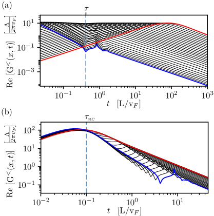
Supplementary Figure 1: Dependence of the Green’s function of a finite wire embedded in a capacative circuit on (a) the discharge time $\tau_{\textrm{\tiny RC}}$ and (b) the length $L$ of the wire. In both cases, the blue lines mark the weak capacitance regime, $\tau_{\textrm{\tiny RC}}/\tau\ll 1$ and the red lines mark the the strong capacitance regime $\tau_{\textrm{\tiny RC}}/\tau\gg 1$. The black curves show how the Green’s function interpolates between the two regimes as the respective paramter is varied. In both plots, interaction strength is fixed at $U/v_{F}=15$.

V TDOS for different wire lengths $L$ and values of $\tau_{\textrm{\tiny RC}}$

In the Sup. Fig. 2 we show the behavior of the tunneling density of states $\nu/\nu_{0}$ for different lengths of the wire, both for vanishing discharge time, i.e., $\tau_{\textrm{\tiny RC}}=0$ [Fig. 2(a-c)] and for finite $\tau_{\textrm{\tiny RC}}$ [Fig. 2(d-f)].

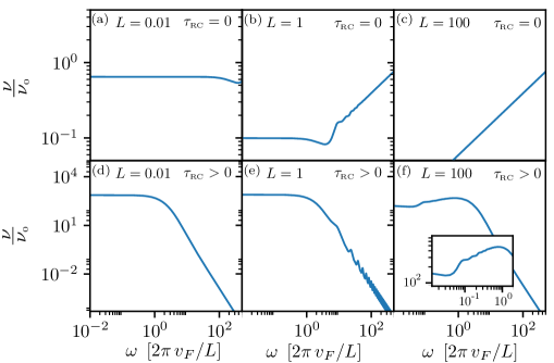
Supplementary Figure 2: The normalized TDOS $\nu/\nu_{0}$ for different lengths $L$ [in units of $v_{F}\,\tau$] of the wire for (a-c) in absence of an external capacative circuit ($\tau_{\textrm{\tiny RC}}=0$) and (d-f) in presence of one ($\tau_{\textrm{\tiny RC}}\neq 0$). The normalization is w.r.t. to the TDOS $\nu_{0}$ in the non-interacting case and in absence of the capacitance, i.e., $\tau_{\textrm{\tiny RC}}=0$. (a) For a short wire, the constant TDOS indicates the free-electron behavior caused by multiple reflections of the plasmons against the boundaries. As $L$ is further decreased, the TDOS $\nu$ will approach $\nu_{0}$. (b) For intermediate lengths, the TDOS shows both free-electron behavior (constant TDOS) at low energies and TLL behavior (power-law growth) at high energies, see Fig. 3(c) in the main text. Furthermore, Fabry-Pérot oscillations with a period of $2\pi/\tau$ appear. (c) For a long wire, the TDOS follows a power-law behavior characteristic for the infinite size TLL-s. In presence of a capacative outer circuit, the TDOS of (d) a short wire is completely determined by the fluctuations with an elevated zero-bias peak and universal $\omega^{-3}$ decay at high energies. (e) At intermediate lengths, the result from the main text is recovered, see Fig. 3(a). Fabry-Pérot oscillations appear at higher energies, but the overall shape is the same as in the case of (d). (f) In case of a long wire, we see that the TDOS for low and high energies behaves as in (d), but in addition an intermediate regime appears, in which the power-law behavior of (b) is recovered [see also the inset of (f)]. This intermediate region is characteristic for the tunneling into a TLL. Throughout, we used a finite interaction strength $U/v_{F}=15$.

References

- Ingold and Nazarov (1992) G.-L. Ingold and Y. V. Nazarov, Charge Tunneling Rates in Ultrasmall Junctions, edited by H. Grabert and M. H. Devoret (Plenum, New York, 1992.).
- Ihn (2004) T. Ihn, Electronic Quantum Transport in Mesoscopic Semiconductor Structures (Springer, 2004).
- Ingold and Nazarov (2005) G.-L. Ingold and Y. V. Nazarov, eprint arXiv:cond-mat/0508728 (2005).
- Josephson (1971) M. Josephson, Japan. J. appl. Phys. 10, 1171 (1971).
- Josephson (1962) B. Josephson, Phys. Lett. 1, 251 (1962).
- Chakravarty and Schmid (1986) S. Chakravarty and A. Schmid, Phys. Rev. B 33, 2000 (1986).
- Kouwenhoven et al. (2001) L. P. Kouwenhoven, D. G. Austing, and S. Tarucha, Reports on Progress in Physics 64, 701 (2001).
- Goldhaber-Gordon et al. (1998) D. Goldhaber-Gordon, H. Shtrikman, D. Mahalu, D. Abusch-Magder, U. Meirav, and M. Kastner, Nature (London) 391, 156 (1998).
- Kouwenhoven and Glazman (2001) L. P. Kouwenhoven and L. Glazman, Phys. World 14, 33 (2001).
- Rössler et al. (2015) C. Rössler, D. Oehri, O. Zilberberg, G. Blatter, M. Karalic, J. Pijnenburg, A. Hofmann, T. Ihn, K. Ensslin, C. Reichl, and W. Wegscheider, Phys. Rev. Lett. 115, 166603 (2015).
- Andreev (1964) A. F. Andreev, Sov. Phys. JETP 19, 1228 (1964).
- van Woerkom et al. (2017) D. J. van Woerkom, A. Proutski, B. van Heck, D. Bouman, J. I. Väyrynen, L. I. Glazman, P. Krogstrup, J. Nygård, L. P. Kouwenhoven, and A. Geresdi, Nature Physics 13, 876 EP (2017).
- Suominen et al. (2017) H. J. Suominen, M. Kjaergaard, A. R. Hamilton, J. Shabani, C. J. Palmstrøm, C. M. Marcus, and F. Nichele, Phys. Rev. Lett. 119, 176805 (2017).
- Das et al. (2012) A. Das, Y. Ronen, Y. Most, Y. Oreg, M. Heiblum, and H. Shtrikman, Nature Physics 8, 887 EP (2012).
- Tomonaga (1950) S. Tomonaga, Prog. Theor. Phys. 5, 544 (1950).
- Luttinger (1963) J. M. Luttinger, J. Math. Phys. 4, 1154 (1963).
- Haldane (1981) F. D. M. Haldane, J. Phys. C: Solid State Phys 14, 2585 (1981).
- Safi and Schulz (1995) I. Safi and H. J. Schulz, Phys. Rev. B 52, R17040 (1995).
- Rosenow et al. (2016) B. Rosenow, I. P. Levkivskyi, and B. I. Halperin, Phys. Rev. Lett. 116, 156802 (2016).
- Auslaender and et al. (2005) O. M. Auslaender and et al., Science 308, 88 (2005).
- Jompol and et al. (2009) Y. Jompol and et al., Science 325, 597 (2009).
- Kane and Fisher (1992a) C. L. Kane and M. P. A. Fisher, Phys. Rev. Lett. 68, 1220 (1992a).
- Matveev and Glazman (1993) K. A. Matveev and L. I. Glazman, Phys. Rev. Lett. 70, 990 (1993).
- Mishchenko et al. (2001) E. G. Mishchenko, A. V. Andreev, and L. I. Glazman, Phys. Rev. Lett. 87, 246801 (2001).
- Gutman et al. (2008) D. B. Gutman, Y. Gefen, and A. D. Mirlin, Phys. Rev. Lett. 101, 126802 (2008).
- Apel and Rice (1982) W. Apel and T. M. Rice, Phys. Rev. B 26, 7063 (1982).
- Giamarchi and Schulz (1988) T. Giamarchi and H. J. Schulz, Phys. Rev. B 37, 325 (1988).
- Vidal et al. (2000) J. Vidal, D. Mouhanna, and T. Giamarchi, International Journal of Modern Physics B, 15 (2000).
- Altland et al. (2012) A. Altland, Y. Gefen, and B. Rosenow, Phys. Rev. Lett. 108, 136401 (2012).
- Altland et al. (2015) A. Altland, Y. Gefen, and B. Rosenow, Phys. Rev. B 92, 085124 (2015).
- Bockrath and et al. (1999) M. Bockrath and et al., Nature 397, 598 (1999).
- Yao and et al. (1999) Z. Yao and et al., Nature 402, 273 (1999).
- Wen (1990) X. G. Wen, Phys. Rev. B 41, 12838 (1990).
- Chang (2003) A. M. Chang, Rev. Mod. Phys. 75, 1449 (2003).
- Ji et al. (2003) Y. Ji, Y. C. Chung, D. Sprinzak, M. Heiblum, D. Mahalu, and H. Shtrikman, Nature(London) 422, 415 (2003).
- Blumenstein and et al. (2011) C. Blumenstein and et al., Nat. Phys. 7, 776 (2011).
- Krinner et al. (2015) S. Krinner, D. Stadler, D. Husmann, J. Brantut, and T. Esslinger, Nature 517, 64 (2015).
- Giamarchi (2003) T. Giamarchi, Quantum Physics in One dimension (Clarendon Press, 2003).
- Levkivskyi (2012) I. Levkivskyi, Mesoscopic Quantum Hall Effect (Springer-Verlag Berlin Heidelberg, 2012.).
- Gutman et al. (2009) D. B. Gutman, Y. Gefen, and A. D. Mirlin, Phys. Rev. B 80, 045106 (2009).
- Gutman et al. (2010) D. B. Gutman, Y. Gefen, and A. D. Mirlin, Phys. Rev. B 81, 085436 (2010).
- Eggert et al. (1996) S. Eggert, H. Johannesson, and A. Mattsson, Phys. Rev. Lett. 76, 1505 (1996).
- Schneider et al. (2008) I. Schneider, A. Struck, M. Bortz, and S. Eggert, Phys. Rev. Lett. 101, 206401 (2008).
- Nazarov et al. (1997) Y. V. Nazarov, A. A. Odintsov, and D. V. Averin, EPL (Europhysics Letters) 37, 213 (1997).
- Slobodeniuk et al. (2013) A. O. Slobodeniuk, I. P. Levkivskyi, and E. V. Sukhorukov, Phys. Rev. B 88, 165307 (2013).
- Kane and Fisher (1992b) C. L. Kane and M. P. A. Fisher, Phys. Rev. B 46, 15233 (1992b).
- Matveev et al. (2010) K. A. Matveev, A. V. Andreev, and M. Pustilnik, Phys. Rev. Lett. 105, 046401 (2010).
- Pothier et al. (1997) H. Pothier, S. Guéron, N. O. Birge, D. Esteve, and M. H. Devoret, Phys. Rev. Lett. 79, 3490 (1997).
- Anthore et al. (2003) A. Anthore, F. Pierre, H. Pothier, and D. Esteve, Phys. Rev. Lett. 90, 076806 (2003).
- Luther and Peschel (1974) A. Luther and I. Peschel, Phys. Rev. B 9, 2911 (1974).
- Fisher and Glazman (1997) M. P. A. Fisher and L. I. Glazman, “Transport in a one-dimensional luttinger liquid,” in Mesoscopic Electron Transport, edited by L. L. Sohn, L. P. Kouwenhoven, and G. Schön (Springer Netherlands, 1997) pp. 331–373.
- Lifshitz and Pitaevskii (1980) E. M. Lifshitz and L. P. Pitaevskii, Statistical Physics, Part 2, Landau and Lifshitz Course of Theoretical Physics Vol. 9 (Butterworth/Heinemann, Oxford, 1980).
- Bruus and Flensberg (2004) H. Bruus and K. Flensberg, Many-Body Quantum Theory in Condensed Matter Physics: An Introduction (Oxford University, Oxford, 2004.).
- von Delft and Schoeller (1998) J. von Delft and H. Schoeller, Annalen Phys. 7, 225 (1998).
- Machlup (1954) S. Machlup, Journal of Applied Physics 25, 341 (1954).
- Carmi and Oreg (2012) A. Carmi and Y. Oreg, Phys. Rev. B 85, 045325 (2012).
- Shahmoon and Leonhardt (2018) E. Shahmoon and U. Leonhardt, Science Advances 4 (2018).
- Note (4) The spatial dependence we discuss in this letter is different than that of a wire with open boundaries [Ref. Eggert et al. (1996)].
- (59) See Supplementary Material for additional details.
- Note (2) In Ref. Nazarov et al. (1997); Safi and Schulz (1995); Gutman et al. (2009), the interaction-dependent scattering amplitudes at the boundary of the wire that enter Eq. (9) were derived microscopically. Our results correspond to the sharp boundary limit of Ref. Gutman et al. (2009) where the reflection coefficient is .
- Cazalilla (2011) M. A. Cazalilla, Reviews of Modern Physics 83, 1405 (2011).
- Yang et al. (2017) B. Yang, Y.-Y. Chen, Y.-G. Zheng, H. Sun, H.-N. Dai, X.-W. Guan, Z.-S. Yuan, and J.-W. Pan, Phys. Rev. Lett. 119, 165701 (2017).
- Giamarchi (2017) T. Giamarchi, Physics 10, 115 (2017).
- Gullans et al. (2016) M. J. Gullans, J. D. Thompson, Y. Wang, Q.-Y. Liang, V. Vuletić, M. D. Lukin, and A. V. Gorshkov, Phys. Rev. Lett. 117, 113601 (2016).
Supplemental Material for

References

- (1) E. G. Idrisov, I. P. Levkivskyi and E. V. Sukhorukov, Phys. Rev. B, 96, 155408 (2017).
- (2) I. S. Gradshteĭn and I. M. Ryžik, Table of Integrals, Series, and Products, 8th Edition, (Academic Press, 2004).
- (3) Y. V. Nazarov, A. A. Odintsov and D. V. Averin, EPL (Europhysics Letters) 37, 213 (1997)