Projected Newton method for a system of Tikhonov-Morozov equations

Abstract

In this paper we derive a Newton type method to solve the non-linear system formed by combining the Tikhonov normal equations and Morozov’s discrepancy principle. We prove that by placing a bound on the step size of the Newton iterations the method will always converge to the solution. By projecting the problem onto a low dimensional Krylov subspace and using the method to solve the projected non-linear system we show that we can reduce the computational cost of the method.

68Q25, 68R10, 68U05

1 Introduction

In this paper we consider linear inverse problems of the form $Ax=b$ with $A\in\mathbb{R}^{m\times n}$, $x\in\mathbb{R}^{n}$ and $b\in\mathbb{R}^{m}$. Here, the right hand side $b$ is the perturbed version of the unknown exact measurements or observations $b_{ex}=b+e$, with $e\sim\mathcal{N}(0,\sigma^{2}I_{m})$. It is well known that for ill-posed problems some form of regularization has to be used in order to deal with the noise $e$ in the data $b$ and to find a good approximation for the true solution of $Ax=b_{ex}$. One of the most widely used methods to do so is Tikhonov regularization. In its standard from, the Tikhonov solution to the inverse problem is given by

(1) $$x_{\alpha}=\operatorname*{arg\,min}_{x\in\mathbb{R}^{n}}\left\|Ax-b\right\|^{2}+\alpha\left\|x\right\|^{2},$$

where $\alpha>0$ is a regularization parameter and $\left\|\cdot\right\|$ denotes the standard Euclidean norm.

The choice of the regularization parameter is very important since its value has a significant impact on the reconstruction. If, on the one hand, $\alpha$ is chosen too large, focus lies on minimizing the regularization term $\left\|x\right\|^{2}$. The corresponding reconstruction $x_{\alpha}$ will therefore no longer be a good solution for the linear system $Ax=b$, will typically have lost many details and be what is referred to as “oversmoothed”. If, on the other had, $\alpha$ is chosen too small, focus lies on minimizing the residual $\left\|Ax-b\right\|^{2}$. This, however, means that the errors $e$ are not suppressed and that the reconstruction $x_{\alpha}$ will be “overfitted” to the measurements.

Figure 1: Sketch of the L-curve (left) and the D-curve (right). The value for $\alpha$ proposed by the L-curve method is typically slightly larger than the one proposed by the discrepancy principle [10].

One way of choosing the regularization parameter is the L-curve method. If $x_{\alpha}$ is the solution of the Tikhonov problem (1), then the curve $(\left\|Ax_{\alpha}-b\right\|,\left\|x_{\alpha}\right\|)$ typically has a rough “L” shape, see figure 1. Heuristically, the value for the regularization parameter corresponding to the corner of this “L” has been proposed as a good regularization parameter because is balances model fidelity (minimizing the residual) and regularizing the solution (minimizing the regularization term) [1, 10, 12, 11]. The problem with this method is that in order to find this value, the Tikhonov problem has to be solved for many different values of $\alpha$, which can be computationally expensive and inefficient for large scale problems.

Another way of choosing the regularization parameter is Morozov’s discrepancy principle [15]. Here, the regularization parameter is chosen such that

(2) $$\left\|Ax_{\alpha}-b\right\|=\eta\varepsilon$$

with $\varepsilon=\left\|e\right\|$ the size of the error and $1\leq\eta$ a tolerance value. The idea behind this choice is that finding a solution $x_{\alpha}$ with a lower residual can only lead to overfitting. Similarly to the L-curve, we can look at the curve $(\alpha,\left\|Ax_{\alpha}-b\right\|)$, which we’ll refer to as the discrepancy curve or D-curve, see figure 1. If $e\sim\mathcal{N}(0,\sigma^{2}I_{m})$, then it is an easy verification to see that $\varepsilon\approx\sigma\sqrt{m}$, but in general the size of the error may be unknown.

In this paper we describe a Newton type method that simultaneously updates the solution $x$ and the regularization parameter $\alpha$ such that the Tikhonov problem (1) and Morozov’s discrepancy principle (2) are both satisfied. This is done by combining both equations into one big non-linear system in $x$ and $\alpha$ and solving it using Newton’s method. However, starting from an arbitrary initial estimate, convergence of the classical Newton’s method cannot be guaranteed. In section 2 we prove that by starting from a specific initial estimate and placing a bound on the step size of the Newton updates the method will always converge. We also derive an estimate for this step size. For large scale problems computing the Newton search directions and this step size can, however, be computationally expensive. In section 4 we therefore combine our method with a projection onto a low dimensional Krylov subspace. In sections 3 and 6 we perform extensive numerical experiments in order to illustrate the workings of these methods and compare them with other regularization methods found in the literature, see section 5. Finally, in section 7, we end the paper with a short discussion on some open questions that remain.

2 Tikhonov-Morozov system

In order to find $(x,\alpha)\in\mathbb{R}^{n}\times\mathbb{R}_{0}^{+}$ that solves the Tikhonov problem and satisfies the discrepancy principle, we consider the non-linear system

(3) $$\left\{\begin{aligned} F_{1}(x,\alpha)&=(A^{T}A+\alpha I)x-A^{T}b\\ F_{2}(x,\alpha)&=\frac{1}{2}(Ax-b)^{T}(Ax-b)-\frac{1}{2}\varepsilon^{2}\end{aligned}\right.$$

for $F:\mathbb{R}^{n}\times\mathbb{R}_{0}^{+}\longmapsto\mathbb{R}^{n}\times\mathbb{R}_{0}^{+}$. Here, $F_{1}(x,\alpha)=0$ are the normal equations corresponding to the Tikhonov problem (1) with regularization parameter $\alpha$ and $F_{2}(x,\alpha)=0$ is equivalent to Morozov’s discrepancy principle (2) (for simplicity we assume that $\eta=1)$.

If we apply Newton’s method to solve this non-linear system of equations, convergence of the method starting from an arbitrary initial estimate cannot be guaranteed. We will prove that by starting from a point $(x_{0},\alpha_{0})$ satisfying the Tikhonov normal equations $F_{1}$, we can guarantee convergence of Newton’s method by limiting the step size. The idea behind this approach is the observation that for points which “almost” satisfy these equations, the Jacobian will be invertible. By placing a bound on the Newton step size, we can force the iterations to remain within this region of interest and prove convergence.

2.1 Newton iterations

If the current Newton iteration for the solution of (3) is given by $\left(x_{k-1},\alpha_{k-1}\right)$, then we write the next iteration as

$$x_{k}=x_{k-1}+\Delta x_{k}\qquad\text{and}\qquad\alpha_{k}=\alpha_{k-1}+\Delta\alpha_{k}.$$

The Jacobian system for the Newton search directions is now given by

$$\begin{pmatrix}A^{T}A+\alpha_{k-1}I&x_{k-1}\\ (Ax_{k-1}-b)^{T}A&0\end{pmatrix}\begin{pmatrix}\Delta x_{k}\\ \Delta\alpha_{k}\end{pmatrix}=-\begin{pmatrix}(A^{T}A+\alpha_{k-1}I)x_{k-1}-A^{T}b\\ \frac{1}{2}(Ax_{k-1}-b)^{T}(Ax_{k-1}-b)-\frac{1}{2}\epsilon^{2}\end{pmatrix},$$

or in short

(4) $$J(x_{k-1},\alpha_{k-1})\begin{pmatrix}\Delta x_{k}\\ \Delta\alpha_{k}\end{pmatrix}=-F(x_{k-1},\alpha_{k-1}).$$

Lemma 2.1.

For all Newton iterations with $k\in\mathbb{N}_{0}$, the following relationship holds:

$$F(x_{k},\alpha_{k})=\begin{pmatrix}\Delta\alpha_{k}\Delta x_{k}\\ \frac{1}{2}\Delta x_{k}^{T}A^{T}A\Delta x_{k}\end{pmatrix}.$$

Proof 2.2.

Using the definition of $F$, it is a straightforward calculation to find that

$$F(x_{k},\alpha_{k})= F(x_{k-1}+\Delta x_{k},\alpha_{k-1}+\Delta\alpha_{k})$$

$$= J(x_{k-1},\alpha_{k-1})\begin{pmatrix}\Delta x_{k}\\ \Delta\alpha_{k}\end{pmatrix}+F(x_{k-1},\alpha_{k-1})+\begin{pmatrix}\Delta\alpha_{k}\Delta x_{k}\\ \frac{1}{2}\Delta x_{k}^{T}A^{T}A_{k}\Delta x\end{pmatrix}.$$

Because the search directions $\Delta x_{k}$ and $\Delta\alpha_{k}$ are found by solving (4), the sum of first two terms equals zero, proving the lemma.

This lemma implies that

(5) $$J(x_{k},\alpha_{k})\begin{pmatrix}\Delta x_{k+1}\\ \Delta\alpha_{k+1}\end{pmatrix}=-\begin{pmatrix}\Delta\alpha_{k}&0\\ \frac{1}{2}\Delta x_{k}^{T}A^{T}A&0\end{pmatrix}\begin{pmatrix}\Delta x_{k}\\ \Delta\alpha_{k}\end{pmatrix},$$

resulting in a recurrence relation between two sequential Newton search directions. Another consequence of the lemma is that

(6) $$\left(A^{T}A+\alpha_{k}I\right)x_{k}-A^{T}b =\Delta\alpha_{k}\Delta x_{k}$$

$$\Leftrightarrow A^{T}\left(Ax_{k}-b\right) =-\alpha_{k}x_{k}+\Delta\alpha_{k}\Delta x_{k}.$$

This means that if we rescale the last row of (4) with $\alpha_{k-1}>0$ and instead solve

$$\begin{pmatrix}A^{T}A+\alpha_{k-1}I&x_{k-1}\\ \frac{1}{\alpha_{k-1}}(Ax_{k-1}-b)^{T}A&0\end{pmatrix}\begin{pmatrix}\Delta x_{k}\\ \Delta\alpha_{k}\end{pmatrix}$$

$$\hskip 70.0001pt=-\begin{pmatrix}(A^{T}A+\alpha_{k-1}I)x_{k-1}-A^{T}b\\ \frac{1}{2\alpha_{k-1}}(Ax_{k-1}-b)^{T}(Ax_{k-1}-b)-\frac{1}{2\alpha_{k-1}}\epsilon^{2}\end{pmatrix},$$

then the same search directions are found and (5) and (6) remain valid.

2.2 At the discrepancy curve

Assume we have $\alpha>0$ and $x$ such that $F_{1}(x,\alpha)=0$. This means that $x$ is the solution of the Tikhonov normal equations

$$(A^{T}A+\alpha I)x=A^{T}b\ \Leftrightarrow\ \frac{1}{\alpha}(Ax-b)^{T}A=-x^{T}$$

and $\left(\alpha,\left\|Ax-b\right\|\right)$ is a point on the discrepancy curve, but not necessarily corresponding to the optimal value of the regularization parameter. In this case, the rescaled Jacobian matrix for the Newton system has the following simplified form:

$$D(x,\alpha):=\begin{pmatrix}A^{T}A+\alpha I&x\\ -x^{T}&0\end{pmatrix}.$$

We now look at the numerical range [7], which for a matrix $A\in\mathbb{C}^{n\times n}$ is defined as

$$W(A)=\left\{\left.\frac{x^{*}Ax}{x^{*}x}\ \right|\ x\in\mathbb{C}^{n},x\neq 0\right\},$$

where $x^{*}$ denotes the complex conjugate of $x$. This is a useful tool since it contains the spectrum of the matrix and for $D(x,\alpha)\in\mathbb{R}^{(n+1)\times(n+1)}$ we find that

$$\begin{pmatrix}u^{*}&v^{*}\end{pmatrix}\begin{pmatrix}A^{T}A+\alpha I&x\\ -x^{T}&0\end{pmatrix}\begin{pmatrix}u\\ v\end{pmatrix}=u^{*}(A^{T}A+\alpha I)u+u^{*}xv-v^{*}x^{T}u$$

with $u\in\mathbb{C}^{n}$, $v\in\mathbb{C}$ and $\left(u^{T},v^{T}\right)^{T}\neq 0$. Since $\alpha>0$ and $x\in\mathbb{R}^{n}$, the first term is strictly positive and real and the last two terms add up to a pure imaginary number. This means that $\forall z\in W(D):real(z)>0$, implying that $0$ is not an eigenvalue and hence that $D$ is invertible.

Lemma 2.3.

For any matrix $A\in\mathbb{R}^{m\times n}$, vector $x\in\mathbb{R}^{n}$ and $\alpha>0$ the Schur complement of $D(x,\alpha)$ exists and is given by $s=x^{T}(A^{T}A+\alpha I)^{-1}x\in\mathbb{R}$. If we set $t:=(A^{T}A+\alpha I)^{-1}x\in\mathbb{R}^{n}$, then it follows that the inverse of $D$ is given by

$$D^{-1}(x,\alpha)=\begin{pmatrix}(A^{T}A+\alpha I)^{-1}-\frac{t^{T}t}{s}&-\frac{t}{s}\\ \frac{t^{T}}{s}&\frac{1}{s}\end{pmatrix}$$

and that the norm of this matrix is bounded:

(7) $$\left\|D^{-1}\right\|\leq\left(1+\frac{\left\|x\right\|}{\alpha}\right)^{2}\max\left\{\frac{1}{\alpha},\frac{\alpha+\lambda_{1}}{\left\|x\right\|}\right\}.$$

Here, $\lambda_{1}$ is the largest eigenvalue of $A^{T}A$.

Proof 2.4.

First note that since $A^{T}A$ is positive semi-definite, the eigenvalues are given by $\lambda_{1}\geq\lambda_{2}\geq\ldots\geq\lambda_{n}\geq 0$. This means that $\left(A^{T}A+\alpha I\right)$ is invertible because it has eigenvalues $\lambda_{1}+\alpha\geq\lambda_{2}+\alpha\geq\ldots\geq\lambda_{n}+\alpha>0$. As a result, the Schur complement of $D$ exists and the formula for $D^{-1}$ can easily be verified, see for example [27]. It now also follows that the eigenvalues of $\left(A^{T}A+\alpha I\right)^{-1}$ are given by

$$\frac{1}{\alpha+\lambda_{n}}\geq\frac{1}{\alpha+\lambda_{n-1}}\geq\ldots\geq\frac{1}{\alpha+\lambda_{1}}>0$$

and thus that

$$\left\|\left(A^{T}A+\alpha I\right)^{-1}\right\|\leq\frac{1}{\alpha+\lambda_{n}}\leq\frac{1}{\alpha}$$

and

$$\left\|t\right\|\leq\frac{\left\|x\right\|}{\alpha}\quad\text{and}\quad\left\|s\right\|\leq\frac{\left\|x\right\|^{2}}{\alpha}.$$

We now write

$$D^{-1}=\begin{pmatrix}I&-t\\ 0&I\end{pmatrix}\begin{pmatrix}\left(A^{T}A+\alpha I\right)^{-1}&0\\ 0&\frac{1}{s}\end{pmatrix}\begin{pmatrix}I&0\\ t^{T}&I\end{pmatrix}$$

and will estimate a bound on the norm of all three matrices. For the first matrix we find that for any unit vector $\left(u^{T},v^{T}\right)^{T}\in\mathbb{R}^{n}\times\mathbb{R}$:

$$\left\|\begin{pmatrix}I&-t\\ 0&I\end{pmatrix}\begin{pmatrix}u\\ v\end{pmatrix}\right\| =\left\|\begin{pmatrix}u-tv\\ v\end{pmatrix}\right\|$$

$$\leq\sqrt{u^{T}u-2u^{T}tv+v^{2}t^{T}t+v^{2}}$$

$$\leq\sqrt{1+2\left\|t\right\|+\left\|t\right\|^{2}}$$

$$\leq\sqrt{\left(1+\left\|t\right\|\right)^{2}}$$

$$\leq 1+\frac{\left\|x\right\|}{\alpha}$$

Analogously, the same bound can be found for the third matrix. For the second matrix we have that

$$\left\|\begin{pmatrix}\left(A^{T}A+\alpha I\right)^{-1}&0\\ 0&\frac{1}{s}\end{pmatrix}\right\|=\max\left\{\left\|\left(A^{T}A+\alpha I\right)^{-1}\right\|,\frac{1}{s}\right\}.$$

It now follows from the min-max theorem [26] that

$$s=x^{T}\left(A^{T}A+\alpha I\right)^{-1}x\geq\frac{\left\|x\right\|}{\alpha+\lambda_{1}}.$$

Combining all these results proves the lemma.

2.3 Step size

We already showed that for points on the discrepancy curve, the inverse Jacobian exists and has a bounded norm. However, even when we start from a point on the discrepancy curve, there is no guarantee that the Newton iterations will remain on this curve. Hence, we are not certain that the linear systems for the Newton update will not become singular. In order to avoid this, we will consider two conditions which are sufficient for the Newton iterations to converge:

1. The inverse Jacobian exists in the next iteration $(x_{k},\alpha_{k})$.

2. The size of the Newton search direction $\left\|\left(\Delta x_{k}^{T},\Delta\alpha_{k}\right)^{T}\right\|$ decreases.

We now show that by placing a bound on the step size of the Newton iterations both conditions can be fulfilled.

In order to derive this bound, we write the Jacobian in any point as a perturbed version of the matrix $D$ using (6):

(8) $$J(x_{k},\alpha_{k})= \begin{pmatrix}A^{T}A+\alpha_{k}I&x_{k}\\ -x_{k}+\frac{\Delta\alpha_{k}}{\alpha_{k}}\Delta x_{k}&0\end{pmatrix}$$

$$= \begin{pmatrix}A^{T}A+\alpha_{k-1}I&x_{k-1}\\ -x_{k-1}^{T}&0\end{pmatrix}+\begin{pmatrix}\Delta\alpha_{k}I&\Delta x_{k}\\ -\frac{\alpha_{k-1}}{\alpha_{k-1}+\Delta\alpha_{k}}\Delta x_{k}^{T}&0\end{pmatrix}.$$

We also replace the Newton updates with a scaled version

$$x_{k}=x_{k-1}+\gamma_{k}\Delta x_{k}\qquad\text{and}\qquad\alpha_{k}=\alpha_{k-1}+\gamma_{k}\Delta\alpha_{k}$$

with

$$\gamma_{k}\in I_{k}:=\left\{\begin{aligned} &\left]0,1\right]&&\text{if }\Delta\alpha_{k}>0\\ &\left]0,1\right]&&\text{if }\Delta\alpha_{k}<0\text{ and }\alpha_{k-1}+\Delta\alpha_{k}>0\\ &\left]0,-\omega\alpha_{k-1}/\Delta\alpha_{k}\right]&&\text{if }\Delta\alpha_{k}<0\text{ and }\alpha_{k-1}+\Delta\alpha_{k}<0\end{aligned}\right.$$

and a tolerance value $\omega\in]0,1[$. This is to ensure that the iterates for $\alpha_{k}$ remain positive and the reason why we consider three different cases will become clear in lemma 2.11. This means that (8) becomes

$$J(x_{k},\alpha_{k})=\underbrace{\begin{pmatrix}A^{T}A+\alpha_{k-1}I&x_{k-1}\\ -x_{k-1}^{T}&0\end{pmatrix}}_{D_{k-1}^{-1}:=}+\underbrace{\gamma_{k}\begin{pmatrix}\Delta\alpha_{k}I&\Delta x_{k}\\ -\zeta_{k}\Delta x_{k}^{T}&0\end{pmatrix}}_{E_{k}:=}.$$

with $\zeta_{k}=\alpha_{k-1}/(\alpha_{k-1}+\gamma_{k}\Delta\alpha_{k})$. We also define the matrix

$$M_{k}:=\gamma_{k}\begin{pmatrix}\Delta\alpha_{k}I&0\\ \frac{1}{2}\Delta x_{k}^{T}A^{T}A&0\end{pmatrix}.$$

Note that we have already shown that $D_{k-1}=D(x_{k-1},\alpha_{k-1})$ has a bounded inverse, so we can use the following theorem:

Theorem 2.5 (Trefethen and Embree).

Suppose D has a bounded inverse $D^{-1}$, then for any $E$ with $\left\|E\right\|<1/\left\|D^{-1}\right\|$, $D+E$ has a bounded inverse $(D+E)^{-1}$ satisfying

$$\left\|(D+E)^{-1}\right\|\leq\frac{\left\|D^{-1}\right\|}{1-\left\|E\right\|\left\|D^{-1}\right\|}$$

Conversely, for any $\mu>1/\left\|D^{-1}\right\|$, there exists an $E$ with $\left\|E\right\|<\mu$ such that $(D+E)u=0$ for some non zero $u$.

Proof 2.6.

For a proof of this theorem we refer to [21, p. 28].

Lemma 2.7.

For the matrices $E_{k},M_{k}\in\mathbb{R}^{(n+1)\times(n+1)}$ defined above, the following holds:

$$\left\|E_{k}\right\| \leq\gamma_{k}\left(\left|\Delta\alpha_{k}\right|+\sqrt{1+\zeta_{k}^{2}}\left\|\Delta x_{k}\right\|\right)$$

$$\left\|M_{k}\right\| =\gamma_{k}\sqrt{\Delta\alpha_{k}^{2}+\frac{1}{4}\left\|A^{T}A\Delta x_{k}\right\|^{2}}.$$

As a consequence we have that

$$\lim_{\gamma_{k}\rightarrow 0}\left\|E_{k}\right\|=0\qquad\text{and}\qquad\lim_{\gamma_{k}\rightarrow 0}\left\|M_{k}\right\|=0.$$

Proof 2.8.

Using the triangle inequality we find that

$$\left\|E_{k}\right\|\leq\gamma_{k}\left(\left\|\begin{pmatrix}\Delta\alpha_{k}I&0\\ 0&0\end{pmatrix}\right\|+\left\|\begin{pmatrix}0&\Delta x_{k}\\ -\zeta_{k}\Delta x_{k}^{T}&0\end{pmatrix}\right\|\right).$$

The first matrix is a diagonal matrix with entries $\Delta\alpha_{k}$ and $0$, hence its norm is equal to $\left|\Delta\alpha_{k}\right|$. For the second matrix we take $u\in\mathbb{R}^{n}$ and $v\in\mathbb{R}$ and find that

$$\left\|\begin{pmatrix}0&\Delta x_{k}\\ -\zeta_{k}\Delta x_{k}^{T}&0\end{pmatrix}\begin{pmatrix}u\\ v\end{pmatrix}\right\| =\left\|\begin{pmatrix}\Delta x_{k}v\\ -\zeta_{k}\Delta x_{k}^{T}u\end{pmatrix}\right\|=\sqrt{\left\|\Delta x_{k}v\right\|^{2}+\left\|\zeta_{k}\Delta x_{k}^{T}u\right\|^{2}}$$

$$\leq\sqrt{v^{2}+\zeta^{2}\left\|u\right\|^{2}}\left\|\Delta x_{k}\right\|$$

$$\Rightarrow\left\|\begin{pmatrix}0&\Delta x_{k}\\ -\zeta_{k}\Delta x_{k}^{T}&0\end{pmatrix}\right\| \leq\sqrt{1+\zeta^{2}}\left\|\Delta x_{k}\right\|.$$

The statement about $\left\|E_{k}\right\|$ now follows. Similarly, we find for $M_{k}$ that

$$\left\|M_{k}\begin{pmatrix}u\\ v\end{pmatrix}\right\| =\left\|\gamma_{k}\begin{pmatrix}\Delta\alpha_{k}u\\ \frac{1}{2}\Delta x_{k}^{T}A^{T}Au\end{pmatrix}\right\|=\gamma\sqrt{\Delta\alpha_{k}^{2}\left\|u\right\|^{2}+\frac{1}{4}\left\|\Delta x_{k}^{T}A^{T}Au\right\|^{2}}$$

$$\leq\gamma\sqrt{\Delta\alpha_{k}^{2}+\frac{1}{4}\left\|A^{T}A\Delta x_{k}\right\|^{2}}\left\|u\right\|$$

By taking $(u,v)=\frac{1}{\left\|A^{T}A\Delta x_{k}\right\|}(A^{T}A\Delta x_{k},0)$ this is an equality, proving the statement about $\left\|M_{k}\right\|$. Finally, it should be noted that $\lim_{\gamma_{k}\rightarrow 0}\zeta_{k}=1$, so for $\gamma_{k}\rightarrow 0$, the norms of both matrices also go to $0$.

Theorem 2.9.

Starting from an initial point $(x_{0},\alpha_{0})$ satisfying the Tikhonov normal equations $F_{1}(x_{0},\alpha_{0})=0$, there exist $\gamma_{k}\in I_{k}$ such that

(9) $$\left\|E_{k}\right\|\left\|D_{k-1}^{-1}\right\|<1$$

(10) $$\frac{\left\|D_{k-1}^{-1}\right\|}{1-\left\|E_{k}\right\|\left\|D_{k-1}^{-1}\right\|}\left\|M_{k}\right\|<1.$$

Scaling the Newton search direction with such a step size $\gamma_{k}$ is sufficient for the Newton iterations to converge.

Proof 2.10.

If (9) holds, then it follows from theorem 2.5 that the inverse Jacobian $J^{-1}(x_{k},\alpha_{k})=\left(D_{k-1}+E_{k}\right)^{-1}$ exists, fulfilling condition (C1). Furthermore, from the recursion between the Newton updates (5) it also follows that

$$\left\|J^{-1}(x_{k},\alpha_{k})\begin{pmatrix}\Delta\alpha_{k}I&0\\ \frac{1}{2}\Delta x_{k}^{T}A^{T}A&0\end{pmatrix}\right\|<1.$$

is a sufficient condition for (C2) to hold. (10) is simply a stronger version of this condition using the bound on $\left\|J^{-1}(x_{k},\alpha_{k})\right\|$ given by theorem 2.5.

It now remains to be shown that such a $\gamma_{k}$ always exists. Since (10) is equivalent to

$$\left\|M_{k}\right\|\left\|D_{k-1}^{-1}\right\|<1-\left\|E_{k}\right\|\left\|D_{k-1}^{-1}\right\|$$

and the left hand side is positive, (9) is implied by (10). Also, since the left hand side goes to $0$ when $\gamma_{k}\rightarrow 0$ and the right hand side goes to 1, there will always exist $\gamma_{k}\in I_{k}$ fulfilling both criteria. Finally, by starting from a point $(x_{0},\alpha_{0})$ satisfying the Tikhonov normal equations, we know that the inverse Jacobian exists in the first iteration.

From this theorem it follows that as long as $\gamma_{k}$ is chosen small enough, the Newton iterations will converge. Small values will however lead to slow convergence, so we will derive an upper bound for $\gamma_{k}$. In order to do this we will simplify the dependency of the upper bound for $\left\|E_{k}\right\|$ found in lemma 2.7 on $\sqrt{1+\zeta_{k}^{2}}$.

Lemma 2.11.

For all $\omega\in]0,1[$ the following holds:

$$\sqrt{1+\zeta^{2}}\leq\left\{\begin{aligned} &\sqrt{2}&&\text{If }\Delta\alpha_{k}>0\\ &\sqrt{1+\left(\frac{\alpha_{k-1}}{\alpha_{k-1}+\Delta\alpha_{k}}\right)^{2}}&&\text{If }\Delta\alpha_{k}<0\text{ and }\alpha_{k-1}+\Delta\alpha_{k}>0\\ &\sqrt{1+\frac{1}{\left(1-\omega\right)^{2}}}&&\text{If }\Delta\alpha_{k}<0\text{ and }\alpha_{k-1}+\Delta\alpha_{k}<0\end{aligned}\right.$$

Proof 2.12.

Finding an upper bound for

$$\sqrt{1+\zeta^{2}}=\sqrt{1+\left(\frac{\alpha_{k-1}}{\alpha_{k-1}+\gamma_{k}\Delta\alpha_{k}}\right)^{2}}$$

is equivalent to finding a lower bound on $\left|\alpha_{k-1}+\gamma_{k}\Delta\alpha_{k}\right|$.

• If $\Delta\alpha_{k}>0$, then $I_{k}=]0,1]$ and this lower bound is found for $\gamma_{k}=0$.

• If $\Delta\alpha_{k}<0$ and $\alpha_{k-1}+\Delta\alpha_{k}>0$ (meaning that using the unscaled Newton iteration would give a positive regularization parameter), then $I_{k}=]0,1]$ and this lower bound is found for $\gamma_{k}=1$.

• If $\Delta\alpha_{k}<0$ and $\alpha_{k-1}+\Delta\alpha_{k}<0$ (meaning that using the unscaled Newton iteration would give a negative regularization parameter), then $I_{k}=\left]0,-\omega\alpha_{k-1}/\Delta\alpha_{k}\right]$. If $\omega\rightarrow 1$ then $\alpha_{k-1}+\gamma_{k}\Delta\alpha_{k}\rightarrow 0$ and $\sqrt{1+\zeta^{2}}\rightarrow+\infty$. In order to avoid this we take $\omega\in]0,1[$ to stay way from this singularity and find the lower bound for $\gamma_{k}=-\omega\alpha_{k-1}/\Delta\alpha_{k}$.

Substituting these values for $\gamma_{k}$ proves the lemma.

Corollary 2.13.

If $\theta_{k}$ is the bound on $\sqrt{1+\zeta_{k}^{2}}$ from lemma 2.11, then the following step size fulfils the conditions (9) and (10) of theorem 2.9:

$$\gamma_{k}=\min\left\{\max I_{k},\frac{1}{\left(\sqrt{\Delta\alpha_{k}^{2}+\frac{1}{4}\left\|A^{T}A\Delta x_{k}\right\|^{2}}+\left|\Delta\alpha_{k}\right|+\theta_{k}\left\|\Delta x_{k}\right\|\right)\left\|D_{k-1}^{-1}\right\|}\right\}$$

Proof 2.14.

This result is found by replacing $\left\|E_{k}\right\|$, $\left\|M_{k}\right\|$ and $\sqrt{1+\zeta^{2}}$ in (10) by their upperbounds found in lemmas 2.7 and 2.11.

Corollary 2.15.

If $\theta_{k}$ is the bound on $\sqrt{1+\zeta_{k}^{2}}$ from lemma 2.11, then the following step size only fulfils conditions (9) of theorem 2.9:

$$\gamma_{k}=\min\left\{\max I_{k},\frac{1}{\left(\left|\Delta\alpha_{k}\right|+\theta_{k}\left\|\Delta x_{k}\right\|\right)\left\|D_{k-1}^{-1}\right\|}\right\}$$

Proof 2.16.

This result is found by replacing $\left\|E_{k}\right\|$ and $\sqrt{1+\zeta^{2}}$ in (9) by their upperbounds found in lemmas 2.7 and 2.11.

Combining the results from this section leads to algorithm 1.

Algorithm 1 Newton on the Tikhonov-Morozov system (NTM)

1:Choose initial $\alpha_{0}>0$ and solve $F_{1}(x_{0},\alpha_{0})$ for $x_{0}$.

2:for $k=1,\ldots,$ maxiter do

3:     Solve the Jacobian system (4) for $\Delta x_{k}$ and $\Delta\alpha_{k}$.

4:     Calculate $\left\|D^{-1}\right\|$.

5:     Calculate $\theta_{k}$ using lemma 2.11.

6:     Calculate the step size $\gamma_{k}$ using corollary 2.13 or 2.15.

7:     $x_{k}=x_{k-1}+\gamma_{k}\Delta x_{k}$ and $\alpha_{k}=\alpha_{k-1}+\gamma_{k}\Delta\alpha_{k}$.

8:     if $\left\|F(x_{k},\alpha_{k})\right\|<$ tol then

9:         break

10:     end if

11:end for

2.4 Remarks

The reason we consider two possible choices for the step size is because we observed in our numerical experiments that both corollary 2.13 and 2.15 seem to result in a small value for the step size. This is explained by the fact that the constraints placed on $\gamma_{k}$ in theorem 2.9 are stronger than (C1) and (C2) and because we used various overestimations in order to derive an upper bound for $\gamma_{k}$.

Another thing to note is that it might not be necessary to start from a point $(x_{0},\alpha_{0})$ on the discrepancy curve. We use this assumption because it guarantees the existence of the inverse Jacobian in the first iteration. However, as theorem 2.5 suggests, it would be sufficient to start from a point for which the perturbation $E$ in the Jacobian $J$ with respect to $D$ sufficiently small. Instead of choosing an $\alpha_{0}$ and solving $F_{1}(x_{0},\alpha_{0})=0$ for $x_{0}$ exactly, it could suffice to only solve for $x_{0}$ up to a limited precision.

Finally, for large scale problems, solving the Jacobian system (4) and calculating $\left\|D_{k-1}^{-1}\right\|$ becomes computationally very expensive. We could use the upper bound from lemma 2.3 to partially solve this problem, but once again, this will only lead to a smaller step size and slower convergence. These issues will be discussed further on in this paper.

3 Numerical experiments I

To illustrate the method, we look at a problem with a small random matrix $A$ and solution $x$. More precisely, we take $A\in\mathbb{R}^{700\times 500}$ and $x\in\mathbb{R}^{500}$ with i.i.d. entries drawn from the uniform distribution $\mathcal{U}(-1,1)$. Measurements are generated by adding $10\%$ Gaussian noise to the exact right hand side $b_{ex}=Ax$ using $e\sim\mathcal{N}\left(0,\sigma^{2}I_{m}\right)$ with $\sigma=0.10\left\|b_{ex}\right\|/\sqrt{m}$ and setting $b=b_{ex}+e$. For the discrepancy principle, we will approximate the error norm by $\varepsilon=\sigma\sqrt{m}=0.10\left\|b_{ex}\right\|$.

We repeat this experiment $1000$ times and for each run we start with $\alpha_{0}=1$ and solve the Tikhonov normal equations $F_{1}(x_{0},\alpha_{0})=0$ for $x_{0}$. After that, we start the Newton iterations with $\omega=0.9$ and stop when $\left\|F(x_{k},\alpha_{k})\right\|<1\mathrm{e}{-3}$. The results are show in figure 2 and table 1, where case 1 means that corollary 2.13 was used to calcuate the step size and case 2 means that corollary 2.15 was used.

These results indicate that the overestimations used in our analysis of the method lead to a small step size. By using corollary 2.15 and weakening the constraints placed on $\gamma$, the method takes substantially larger steps and converges much faster. How much larger the step sizes can become by weakening the constraints is of course problem dependent and hard to predict. Nevertheless, (C2) seems to be a strong constraint placed on the iterations. Also, because both cases converge to the same solution, the same regularization parameter is found. The small standard deviation over all the runs indicates that the regularization parameter is quite similar in all the runs.

Figure 2: Results for one of the runs. For each Newton iteration, we plot the point $(\alpha_{k},\left\|Ax_{k}-b\right\|)$. The top left figure corresponds to case 1 and the top right figure to case 2. Bottom left: the value of the step size $\gamma$ used in each iteration. Bottom right: the value of the regularization parameter $\alpha$ in each iteration.

	# Iterations	$\alpha$
Case 1	$85$ ($13$)	$15.6581$ ($1.0947$)
Case 2	$16$ ($2$)	$15.6581$ ($1.0947$)

Table 1: Average number of iterations for the 1000 runs of the experiment and the standard deviation (rounded). Because both methods converge to the same solution, the same value for $\alpha$ is found in each run, but for all the different random matrices its value turns out to be quite similar, hence the low standard deviation.

4 Projected Tikhonov-Morozov system

The NTM algorithm can become computationally very expensive because in each iteration $\left\|D^{-1}\right\|$ needs to be computed and the Jacobian system (4) needs to be solved for $\Delta x$ and $\Delta\alpha$. Even for small matrices $A\in\mathbb{R}^{m\times n}$ this can quickly become a problem. However, it is possible to project the problem onto a Krylov subspace [20, 24] using a bidiagonal decomposition of $A$ [8, 18, 17]. In each outer Krylov iteration, the projected version of the Tikhonov-Morozov system (3) can then be solved using the NTM algorithm.

In this section we describe how this algorithm works using a number of heuristic choices and apply it to different test problems. Roughly speaking, each iteration of the method will consist of the following steps:

• Expand the bidiagonal decomposition of $A$.

• Choose an initial point for the NTM method on the projected equations.

• Calculate a number of NTM iterations on the projected equations.

• Check the convergence.

4.1 Bidiagonal decomposition

Theorem 4.1 (Bidiagonal decomposition).

If $A\in\mathbb{R}^{m\times n}$ with $m\geq n$, then there exist orthonormal matrices

$$U=(u_{1},u_{2},\ldots,u_{m})\in\mathbb{R}^{m\times m}\quad\text{and}\quad V=(v_{1},v_{2},\ldots,v_{n})\in\mathbb{R}^{n\times n}$$

and a lower bidiagonal matrix

$$B=\begin{pmatrix}\mu_{1}\\ \nu_{2}&\mu_{2}\\ &\nu_{3}&\ddots\\ &&\ddots&\mu_{n}\\ &&&\nu_{n+1}\end{pmatrix}\in\mathbb{R}^{(n+1)\times n},$$

such that

$$A=U\begin{pmatrix}B\\ 0\end{pmatrix}V^{T}.$$

Proof 4.2.

This was proven by Golub and Kahan in [8].

Starting from a given unit vector $u_{1}\in\mathbb{R}^{m}$ it is possible to generate the columns of $U$, $V$ and $B$ recursively using the Bidiag1 procedure proposed by Paige and Saunders [17, 18], see algorithm 2. Here, the reorthogonalization is added for numerical stability. Note that this bidiagonal decomposition is the basis for the LSQR algorithm and that after $k$ steps of Bidiag1 starting with the initial vector $u_{1}=b/\left\|b\right\|$ we have matrices $V_{k}\in\mathbb{R}^{n\times k}$ and $U_{k+1}\in\mathbb{R}^{m\times(k+1)}$ with orthonormal columns and a lower bidiagonal matrix $B_{k+1,k}\in\mathbb{R}^{(k+1)\times k}$ that satisfy

(11) $$AV_{k}=U_{k+1}B_{k+1,k}$$

Algorithm 2 bidiag1

1:Choose initial unit vector $u_{1}$ (typically $b/\left\|b\right\|$).

2:Set $\nu_{1}v_{0}=\mu_{n+1}v_{n=1}=0$.

3:for $k=1,\ldots,$ n do

4:     $r_{k}=A^{T}u_{k}-\nu_{k}v_{k-1}$

5:     Reorthogonalize $r_{k}$ with respect to the previous columns of $V$.

6:     $\mu_{k}=\left\|r_{k}\right\|$ and $v_{k}=r_{k}/\mu_{k}$.

7:     $p_{k}=Av_{k}-\mu_{k}u_{k}$

8:     Reorthogonalize $p_{k}$ with respect to the previous columns of $U$.

9:     $\nu_{k+1}=\left\|p_{k}\right\|$ and $u_{k+1}=p_{k}/\nu_{k+1}$.

10:end for

In order to solve the Tikhonov-Morozov system (3), we will calculate a series of iterations in the Krylov subspace spanned by the columns of $V$:

$$x_{k}\in\operatorname{span}{V_{k}}=\mathcal{K}_{k}(A^{T}A,A^{T}b).$$

This means that $x_{k}=V_{k}y_{k}$ for some $y_{k}\in\mathbb{R}^{k}$ and using (11), the orthonormality of the columns of $U$ and $V$ and the fact that $u_{1}=b/\left\|b\right\|$ it is possible to show that

(12) $$\min_{x_{k}\in\operatorname{span}{V_{k}}}\left\|Ax_{k}-b\right\|^{2}+\alpha\left\|x_{k}\right\|^{2}=\min_{y_{k}\in\mathbb{R}^{n}}\left\|B_{k+1,k}y_{k}-c_{k}\right\|^{2}+\alpha\left\|y_{k}\right\|^{2}$$

and

(13) $$\left\|Ax_{k}-b\right\|=\left\|B_{k+1,k}y_{k}-c_{k}\right\|,$$

for $c_{k}=(\left\|b\right\|,0,\ldots,0)^{T}\in\mathbb{R}^{k+1}$. We therefore set $x_{k}=V_{k}y_{k}$ and solve the following projected version of (3):

(14) $$\left\{\begin{aligned} \widetilde{F}_{1}(y_{k},\alpha_{k})&=(B_{k+1,k}^{T}B_{k+1,k}+\alpha I_{k})y_{k}-B_{k+1,k}^{T}c_{k}\\ \widetilde{F}_{2}(xy_{k}\alpha_{k})&=\frac{1}{2}\left(B_{k+1,k}y_{k}-c\right)^{T}\left(B_{k+1,k}y_{k}-c_{k}\right)-\frac{1}{2}\varepsilon^{2}\end{aligned}\right.$$

Similarly to the to original non-linear system, $\widetilde{F}_{1}$ are the normal equations corresponding to the projected Tikhonov problem (12) and $\widetilde{F}_{2}$ corresponds to the projected discrepancy principle (13).

4.2 Inner NTM iterations

In each outer Krylov iteration (numbered with $k$) (14) needs to be solved, which we will do using the NTM method. This means that in the inner Newton iterations (numbered with $l$), the following Jacobian system needs to be solved:

(15) $$\begin{pmatrix}B_{k+1,k}^{T}B_{k+1,k}+\alpha_{k,l-1}I_{k}&y_{k,l-1}\\ \frac{1}{\alpha_{k,l-1}}\left(B_{k+1,k}y_{k,l-1}-c_{k}\right)^{T}B_{k+1,k}&0\end{pmatrix}\begin{pmatrix}\Delta y_{k,l}\\ \Delta\alpha_{k,l}\end{pmatrix}$$

$$\qquad\quad=-\begin{pmatrix}\left(B_{k+1,k}^{T}B_{k+1,k}+\alpha_{k,l-1}I_{k}\right)y_{k,l-1}-B_{k+1,k}^{T}c_{k}\\ \frac{1}{2\alpha_{k,l-1}}\left(B_{k+1,k}y_{k,l-1}-c_{k}\right)^{T}\left(B_{k+1,k}y_{k,l-1}-c_{k}\right)-\frac{1}{2\alpha_{k,l-1}}\varepsilon^{2}\end{pmatrix}.$$

Note that the matrix $B_{k+1,k}^{T}B_{k+1,k}$ has size $k\times k$. This means that as long as the number of outer iterations remains small – which corresponds to the size of the constructed Krylov basis – calculating $\left\|D_{l-1}^{-1}\right\|$ and solving the projected Jacobian system (15) of size $(k+1)\times(k+1)$ can be done efficiently. A full overview of the method can be found in algorithm 3 and below we discuss some of the steps.

As a starting point for the original NTM method, we used the solution to the Tikhonov normal equations $F_{1}(x_{0},\alpha_{0})=0$ for a chosen $\alpha_{0}$. Now, in each outer Krylov iteration, we will use the current best estimate for the regularization parameter, i.e. $\alpha_{k,0}=\alpha_{k-1}$ and solve the projected Tikhonov normal equations $\widetilde{F}_{1}(y_{k,0},\alpha_{k,0})$. This $k\times k$ linear system can be solved quickly as long as the number of Krylov iterations is small and its solution can be used to initialize the inner Newton iterations.

Another important question is how many inner Newton iterations should be performed before the Krylov subspace is expanded. If, on the one hand, the Krylov subspace is too small to contain the solution $x$ of the inverse problem (or a good approximation of it), then the Newton iterations cannot converge. Therefore we would like the number of inner iterations to be small. If, on the other hand, the Krylov subspace is large enough to contain the solution, we don’t want to keep expanding it. The maximum number of inner Newton iterations should therefore be large enough for them to converge. This is why we initially limit the number of inner Newton iterations. However, the moment that the residual of the solution becomes less than the discrepancy level $\varepsilon$, we will take a much larger number. This corresponds to lines 6–10 of algorithm 3.

Finally, we don’t change the stopping criterion for the inner Newton iterations, algorithm 3 line 16. However, because we are now working with the the projected system, $\widetilde{F}$ may be solved accurately before the original system $F$ is. We therefore don’t stop the outer Krylov iterations until the value for the regularization parameter $\alpha_{k}$ stagnates as well, algorithm 3 line 22. The necessity for this will become clear in the numerical experiments, where we will see that this corresponds to finding a solution $x_{k}$ that satisfied the discrepancy principle, but not the Tikhonov normal equations.

Algorithm 3 Projected Newton on the Tikhonov-Morozov system (PNTM)

1:Choose initial $\alpha_{0}>0$.

2:Set FLAG $=0$.

3:for $k=1,\ldots,$ outeriter do

4:     Expand $U_{k+1}$, $B_{k+1,k}$ and $V_{k}$ using Bidiag1 (2).

5:     Set $\alpha_{k,0}=\alpha_{k-1}$ and solve $\widetilde{F}_{1}(y_{k,0},\alpha_{k,0})$ for $y_{k,0}$.

6:     if $\left\|B_{k+1,k}y_{k,0}-c_{k}\right\|>\epsilon$ then

7:         inneriter $=\min\left\{k,10\right\}$

8:     else

9:         inneriter $=10000$

10:     end if

11:     for $l=1,\ldots,$ inneriter do

12:         Solve the projected Jacobian system (15) for $\Delta y_{k,l}$ and $\Delta\alpha_{k,l}$.

13:         Calculate $\left\|D^{-1}_{l-1}\right\|$.

14:         Calculate the step size $\gamma$ using corollary 2.13 or 2.15.

15:         $y_{k,l}=y_{k,l-1}+\gamma\Delta y_{k,l}$ and $\alpha_{k,l}=\alpha_{k,l-1}+\gamma\Delta\alpha_{k,l}$.

16:         if $\left\|\widetilde{F}(y_{k,l},\alpha_{k,l})\right\|<$ tol then

17:              FLAG $=1$

18:              break

19:         end if

20:     end for

21:     $x_{k}=V_{k}y_{k,l}$ and $\alpha_{k}=\alpha_{k,l}$.

22:     if FLAG $=1$ and $\left|\alpha_{k}-\alpha_{k-1}\right|/\alpha_{k-1}<$ tol then

23:         break

24:     end if

25:end for

5 Reference methods

In this section we briefly discuss two methods which we compare the PNTM method to. The first method iteratively solves the Tikhonov problem and also uses an iterative update scheme for the regularization parameter based on the discrepancy principle. The second method does not solve the Tikhonov problem, but combines an early stopping criterion with a right preconditioner in order to include prior knowledge and regularization.

5.1 Generalized bidiagonal-Tikhonov

In [4, 5, 6] a generalized Arnoldi-Tikhonov method (GAT) was introduced that iteratively solves the Tikhonov problem (1) using a Krylov subspace method based on the Arnoldi decomposition of the matrix $A$. Simultaneously, after each Krylov iteration, the regularization parameter is updated in order to approximate the value for which the discrepancy is equal to $\varepsilon$. This is done using one step of the secant method to find the intersection of the discrepancy curve with the tolerance for the discrepancy principle, see figure 1, but in the current Krylov subspace. Because the method is based on the Arnoldi decomposition, the method is connected to the GMRES algorithm and it only works for square matrices. However, by replacing the Arnoldi decomposition with the bidiagonal decomposition we used in the previous section the method can be adapted to non-square matrices.

The update for the regularization parameter is done based on the regularized and the non-regularized residual. Let, in the $k$th iteration, $z_{k}$ be the solution without regularization – i.e. $\alpha=0$ – and $y_{k}$ the solution with the current best regularization parameter – i.e. $\alpha=\alpha_{k-1}$. If $r(z_{k})$ and $r(y_{k})$ are the corresponding residuals, then the regularization parameter is updates using

(16) $$\alpha_{k}=\left|\frac{\varepsilon-r(z_{k})}{r(y_{k})-r(z_{k})}\right|\alpha_{k-1}.$$

A brief sketch of this method is given is algorithm 4, where we use the same stopping criterion as for PNTM, but for more information we refer to [4, 5, 6]. Note that in the original GAT method, the non-regularized iterates $z_{k}$ are equivalent to the GMRES iterations for the solution of $Ax=b$. Now, because the Arnoldi decomposition is replaced with the bidiagonal decomposition, they are equivalent to the LSQR iterations for the solution of $Ax=b$.

Algorithm 4 Generalized bidiagonal Tikhonv (GBiT)

1:Choose initial $\alpha_{0}>0$.

2:for k = 1, …, maxiter do

3:     Expand $U_{k+1}$, $B_{k+1,k}$ and $V_{k}$ using Bidiag1 (2).

4:     Solve $\widetilde{F}_{1}(z_{k},0)=0$ for $z_{z}$.

5:     Solve $\widetilde{F}_{1}(y_{k},\alpha_{k-1})=0$ for $y_{k}$.

6:     Calculate $\alpha_{k}$ using (16).

7:     if $\left\|\widetilde{F}(y_{k},\alpha_{k})\right\|<$ tol and $\left|\alpha_{k}-\alpha_{k-1}\right|/\alpha_{k-1}<$ tol then

8:         break

9:     end if

10:end for

5.2 General form Tikhonov and priorconditioning

In its general form, the Tikhonov problem (1) is written as

(17) $$x_{\alpha}=\operatorname*{arg\,min}_{x\in\mathbb{R}^{n}}\left\|Ax-b\right\|^{2}+\alpha\left\|L(x-x_{0})\right\|^{2},$$

with $x_{0}\in\mathbb{R}^{n}$ an initial estimate and $L\in\mathbb{R}^{p\times n}$ a regularization matrix, both chosen to incorporate prior knowledge or to place specific constraints on the solution [4, 11]. If $L$ is a square invertible matrix, then the problem can be written in the standard form

(18) $$z_{\alpha}=\operatorname*{arg\,min}{z\in\mathbb{R}^{n}}\left\|\overline{A}z-r_{0}\right\|^{2}+\alpha\left\|z\right\|^{2},$$

by using the transformation

(19) $$z=L(x-x_{0}),\quad\overline{A}=AL^{-1},\quad r_{0}=b-Ax_{0}.$$

When $L$ is not square invertible, some form of pseudoinverse has to be used, but the reformulation of the problem remains the same [11].

After solving (18), the solution can be found as

$$x=x_{0}+L^{-1}z.$$

Instead of solving $Ax=b$, an alternative regularization method called priorconditionning is to solve

$$\left\{\begin{aligned} &AL^{-1}z=b-Ax_{0}\\ &x=x_{0}+L^{-1}z\end{aligned}\right.$$

Here, the matrix $L$ is can be seen as a right preconditioner. Its functions is, however, not to improve the convergence of the iterative method, but to incorporate regularization and prior knowledge into the solution [2]. This priorconditionned linear system can now be solved with CGLS combined with an early stopping criterion based on the discrepancy principle. Note that this method will find a solution in the same Krylov subspace as PNTM, but that PNTM selects another element of this space due to the presence of the regularization term.

6 Numerical Experiments II

6.1 Large random matrix problem

As a first numerical experiment, we repeat the random matrix experiment from section 3. The only thing we change is the size of the matrices: $21000\times 15000$. The results are shown in figure 3 and table 2, where we used $tol=1\mathrm{e}{-3}$ for the stopping criterion. Similarly as with the smaller experiment, there is little difference between the different runs when it comes to the number of iterations (outer and inner) or the optimal regularization parameter. As a comparison, we also solved the problem with GBiT and see that while a similar value for the regularization parameter is found, PNTM requires less Krylov iterations in order to converge.

When we compare figure 2 and figure 3, we see that the behaviour of the method is quite different now. In the original NTM method we started from a point on the discrepancy curve and stayed close to it by limiting the step size. Now, with the PNTM method, we solve the problem in Krylov subspaces of increasing size. This means that in the first few iterations, we end up far away from the true discrepancy curve. At some point we have constructed a Krylov subspace in which we can solve the projected system up to the discrepancy principle, but as we observe, not necessarily the true Tikhonov normal equations. At this point we increase the maximum number of inner iterations and we keep performing outer Krylov iterations until the regularization parameter stagnates.

Whichever of the two corollaries we use to determine the step size produces similar results. The main difference is the number of inner iterations required to solve the projected system. Using corollary 2.15, the method once again requires a significantly lower number of Newton iterations to converge inside each of the Krylov subspaces.

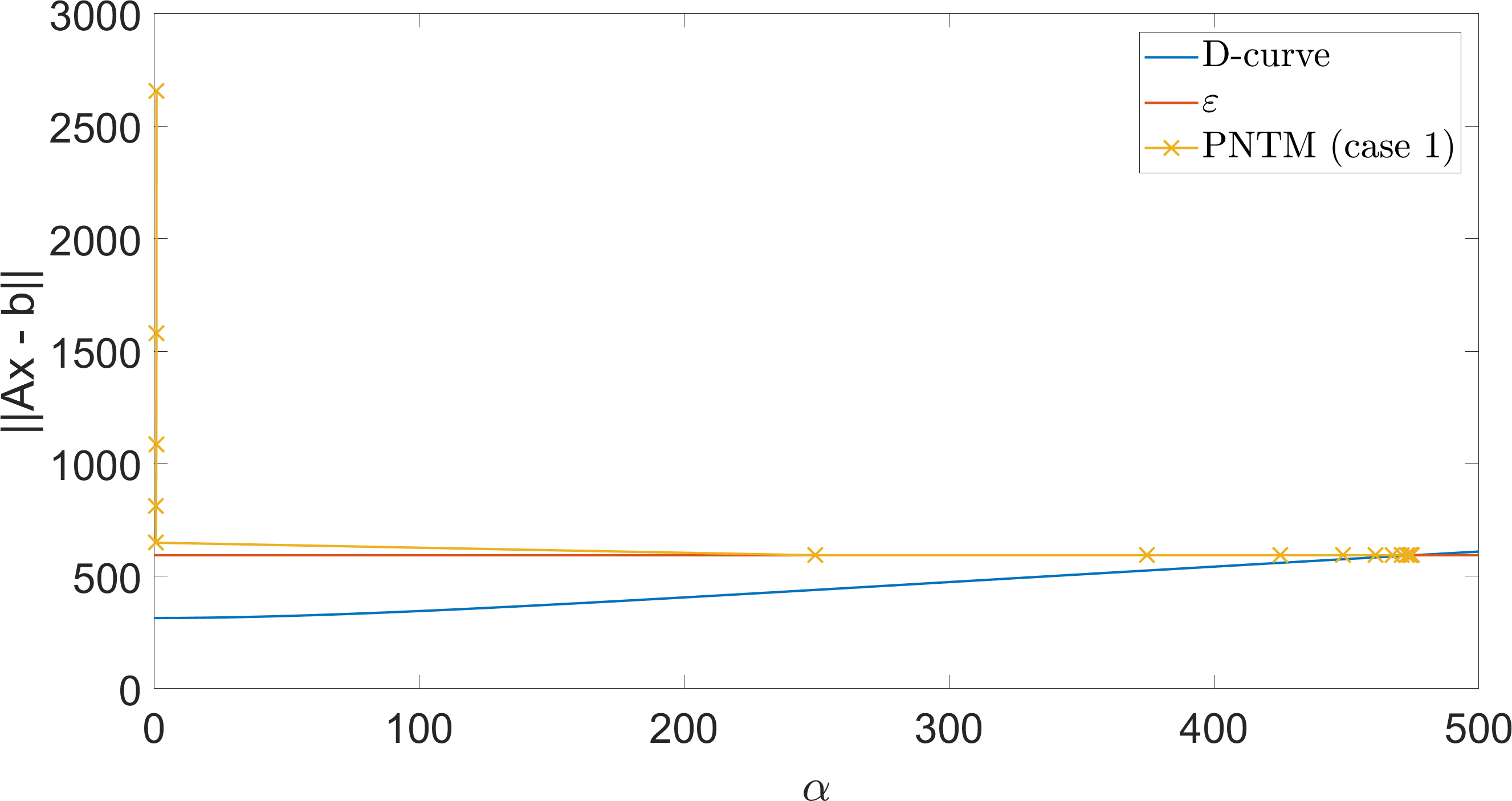
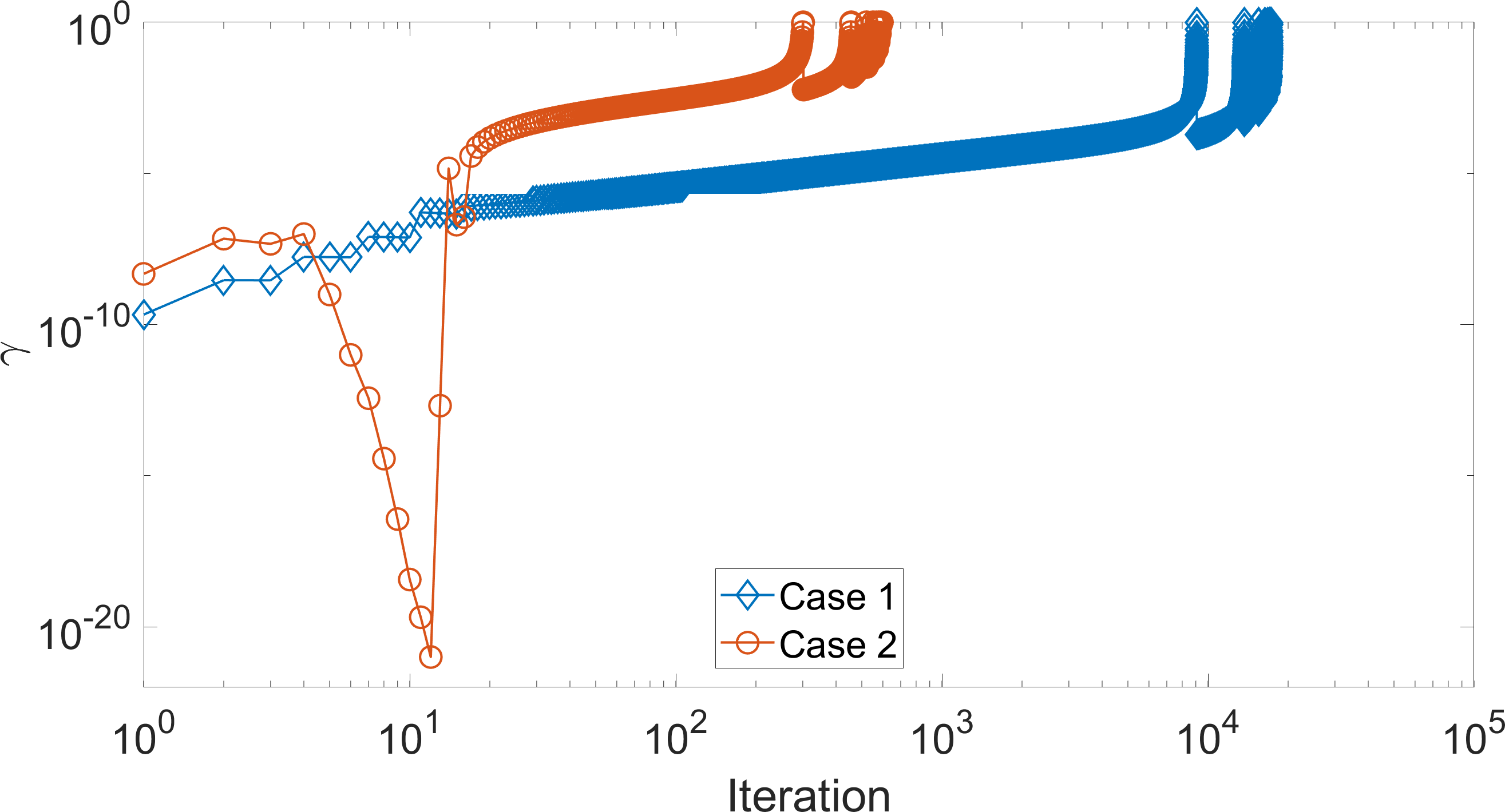
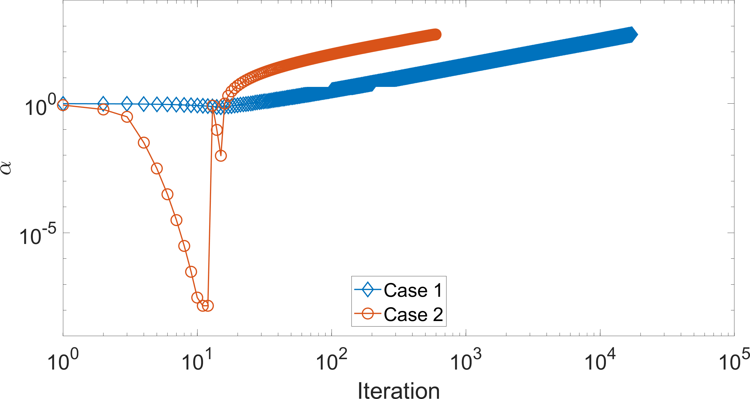
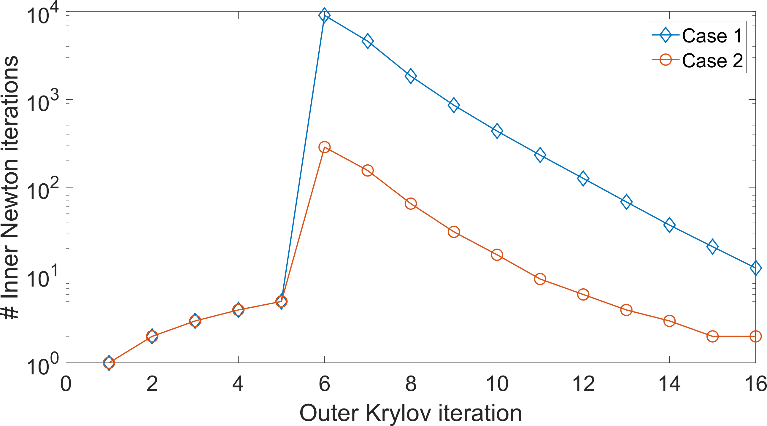
Figure 3: For each Newton iteration, we plot the point $(\alpha_{k},\left\|Ax_{k}-b\right\|)$ to see where it lies with respect to the discrepancy curve. The top left figure corresponds to case 1, the top right figure to case 2. Middle left: the value of the step size used in each iteration. Middle right: the value of the regularization parameter in each iteration. Bottom: the number of inner Newton iterations per outer Krylov iteration.

	# Krylov iterations	# Newton iterations	$\alpha$
PNTM – case 1	$16$ ($<1$)	$16772$ ($432$)	$469.0143$ ($5.98$)
PNTM – case 2	$16$ ($<1$)	$576$ ($14$)	$469.0144$ ($5.98$)
GBiT	$32$ ($<1$)	$\cdot$	$469.3934$ ($5.97$)

Table 2: Average number of iterations for the 1000 runs of the experiment and the standard deviation (rounded). The number of outer iterations corresponds to the dimension of the constructed Krylov subspace, whereas the number of inner iterations is the total number of Newton iterations during all the outer iterations. Because both methods converge to the same solution, the same value for $\alpha$ is found in each run, but for all the different random matrices its value turns out to be quite similar, hence the low standard deviation.

6.2 Computed tomography

As a second numerical experiment, we consider x-ray computed tomography. Here, the goal is to reconstruct the attenuation factor of an object based on the loss of intensity in the x-rays after they passed through the object. Classically, the reconstruction is done using analytical methods based on the Fourier and Randon transformations [14]. In the last decades interest has grown in algebraic reconstruction methods due to their flexibility when it comes to incorporating prior knowledge and handling limited data. Here, the problem is written as a linear system $Ax=b$, where $x$ represents the attenuation of the object in each pixel, the right-hand side $b$ is related to the intensity measurements of the x-rays and $A$ is a projection matrix. The precise structure of $A$ depends on the experimental set-up, but it is typically very sparse. For more information we refer to [13, 11, 16]. We also do not construct the matrix $A$ explicitly, but use the ASTRA toolbox [22, 23] in order to calculate the matrix vector products on-the-fly using their GPU implementation [19].

As a test image we take the modified Shepp–Logan phantom of size $512\times 512$ and take $720$ projection angles in $[0,\pi[$, which corresponds to a matrix $A$ of size $(720\cdot 512)\times(512\cdot 512)$. Similar to the previous experiments we add $10\%$ noise to the exact right hand size (resulting here in $\varepsilon=4.3513\mathrm{e}{3}$), but we will only calculate the PNTM reconstruction using the larger step size from corollary 2.15. We also calculate the reconstruction using GBiT and the simultaneous iterative reconstruction technique (SIRT) [9]. The latter is a widely used fixed point iteration method for tomographic reconstructions based on the following recursion:

$$x_{k+1}=x_{k}+CA^{T}R\left(b-Ax_{k}\right).$$

Here, $R$ and $C$ are diagonal matrices whose elements are the inverse row and column sums, i.e. $r_{ii}=1/\sum_{i}a_{ij}$ and $c_{jj}=1/\sum_{i}a_{ij}$. It can also be shown that this algorithm converges to the solution of the following weighted least squares problem:

$$x^{*}=\operatorname*{arg\,min}_{x\in\mathbb{R}^{n}}\left\|Ax-b\right\|_{R}^{2}$$

Note that, on the one hand, just like PNTM or GBiT, each SIRT iteration requires one multiplication with $A$ and one with $A^{T}$. On the other hand, it does not need to construct and store a basis for the Krylov subspace, so it is computationally less expensive and requires much less memory – two main advantages of the method.

The reconstructions are shown in figure 4, with further details in Figure 5 and table 3. Here, we used $tol=1\mathrm{e}{-3}$ for the PNTM and GBiT stopping criterion and stopped the SIRT iterations once the residual was smaller than the discrepancy tolerance $\varepsilon$. Furthermore, because the 2-norm is not always a good measure for how closely two images visually resemble each other, we also consider the structural similarity index (SSIM)[25]. For two images $x$ and $y$ and default values $C_{1}=0.01^{2}$ and $C_{2}=0.03^{2}$, this index is given by:

$$SSIM(x,y)=\frac{\left(2\mu_{x}\mu_{y}+C_{1}\right)\left(2\sigma_{xy}+C_{2}\right)}{\left(\mu_{x}^{2}+\mu_{y}^{2}+C_{1}\right)\left(\sigma_{x}^{2}+\sigma_{y}^{2}+C_{2}\right)}.$$

Here, $\mu_{x}$ and $\mu_{y}$ are the mean intensity of the images, $\sigma_{x}$ and $\sigma_{y}$ their standard deviation and $\sigma_{xy}$ the covariance. This index lies between $0$ and $1$ and the lower its value, the better the image $x$ resembles the reference image $y$.

When we look at the results, we see that there is little difference between the errors of the reconstructions, but that SIRT has a much larger SSIM. When looking at the reconstructed images, we see see that this images is indeed smoother than the others. Because SIRT is a stationary method, it also needs more iterations than PNTM and GBiT, which are both Krylov methods. Similarly as with the previous experiment, however, we see that GBiT needs almost twice as many Krylov iterations as PNTM. When we look at figure 5 we see that while the value for the regularization parameter stagnates at a similar pace, PNTM more quickly minimizes the value of $\widetilde{F}$.

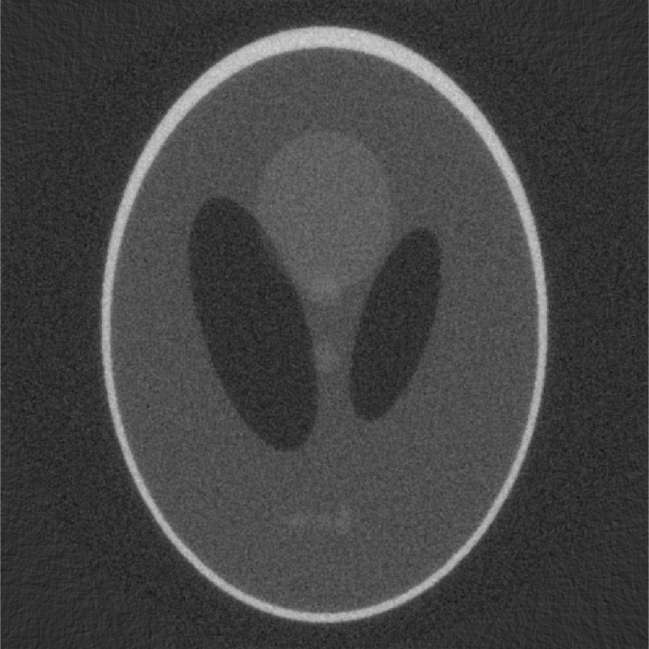
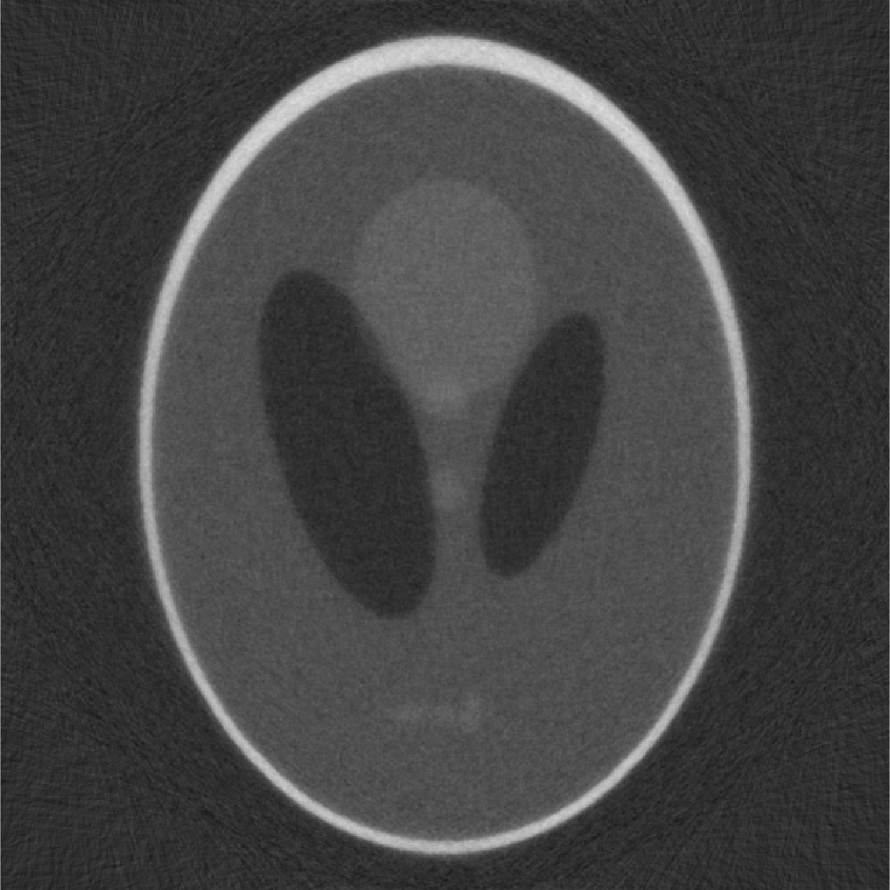
Figure 4: Top: original Shepp-Logan phantom with values in $[0,1]$. Bottom: from left to right the PNTM, GBiT and SIRT reconstructions with values in $[-0.2074,1.0889]$, $[-0.2071,1.0899]$ and $[-0.1477,1.1078]$ respectively. Here, all images are shown on a colorscale $[-0.3,1.3]$.

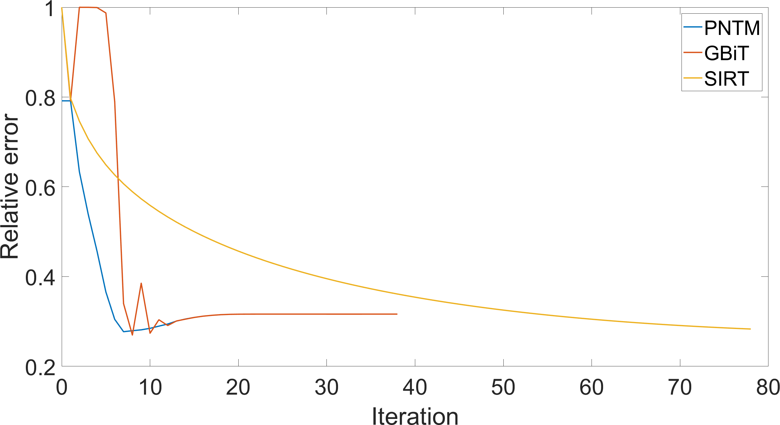
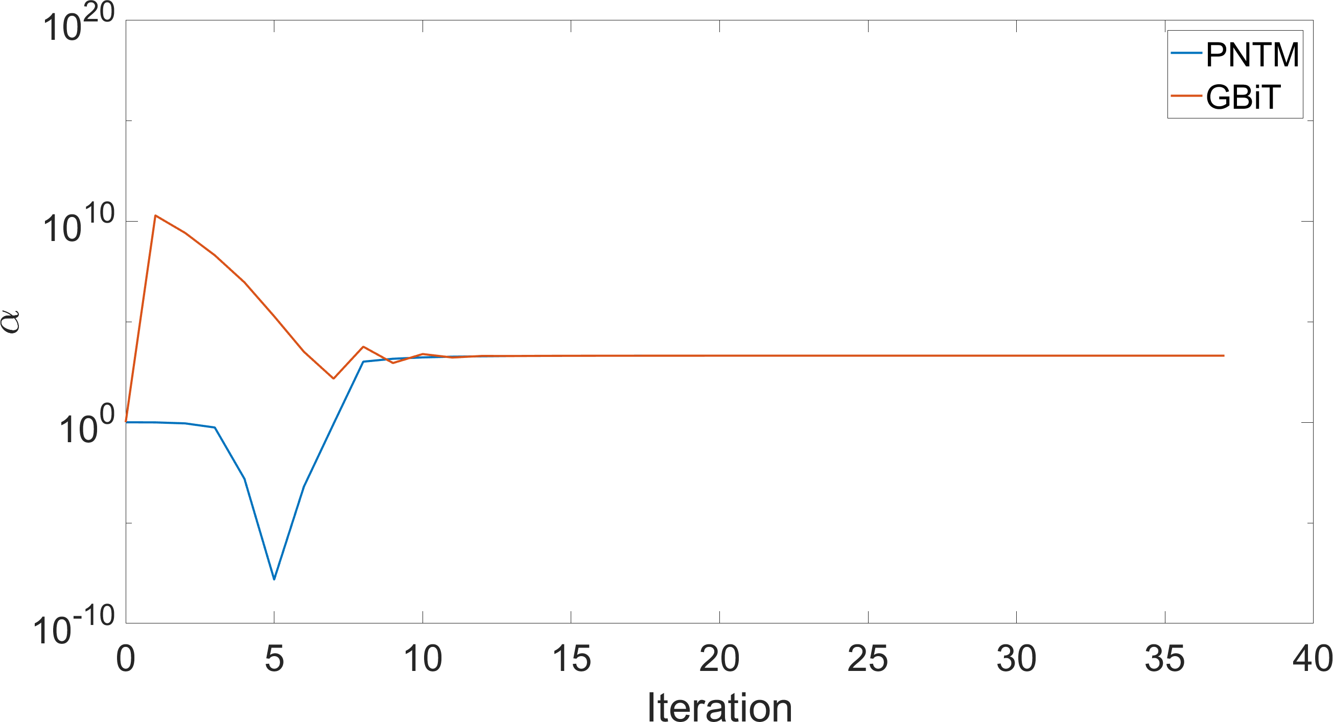
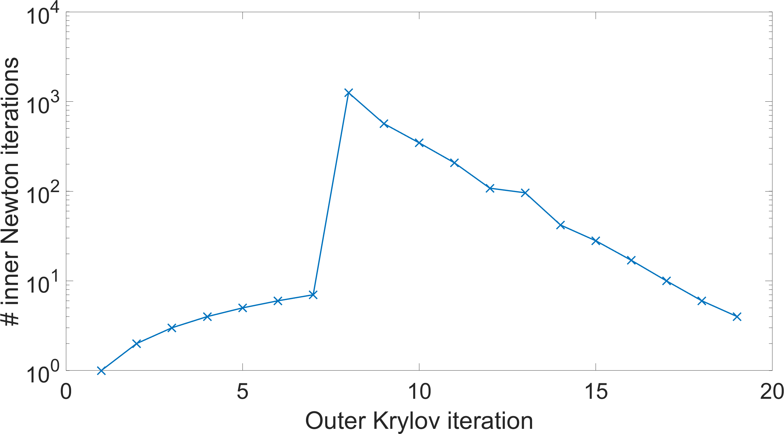
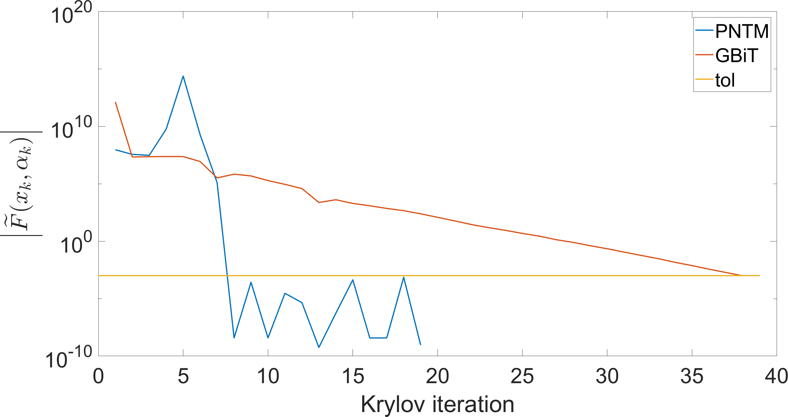
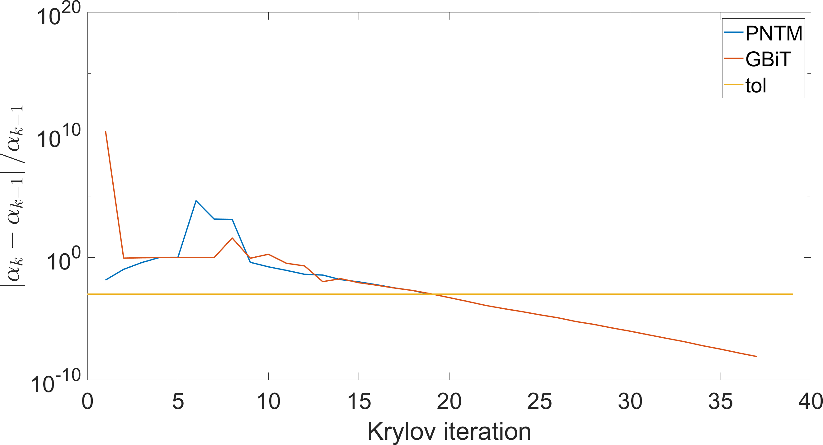
Figure 5: Top: relative error in each iteration. Middle left: value of the regularization parameter in each iteration. Middele right: number of inner Newton iterations in each outer Krylov iterations for PNTM. Bottom: the two parts of the stopping criterion for PNTM and GBiT.

	# Iterations	Relative error	Residual	SSIM	$\alpha$
PNTM	$19$ ($2714$)	$0.3159$	$4.3513\mathrm{e}{3}$	$0.2507$	$2.0399\mathrm{e}{3}$
GBiT	$38$	$0.3164$	$4.3513\mathrm{e}{3}$	$0.2499$	$2.0413\mathrm{e}{3}$
SIRT	$78$	$0.2832$	$4.3443\mathrm{e}{3}$	$0.4117$	$\cdot$

Table 3: Details from the CT reconstructions. The Krylov method PNTM and GBiT require less iterations than SIRT, but again PNTM needs less iterations than GBiT. While the relative error is very similar, the SIRT reconstruction has a much larger SSIM. The total number of inner Newton iterations for PNTM is mentioned in parentheses.

6.3 Suite sparse matrix collection

As a final experiment we take the 26 matrices $A\in\mathbb{R}^{m\times n}$ from the “SuiteSparse Matrix Collection” corresponding to a least squares problem [3]. For each matrix we generate a solution vector $x_{ex}\in\mathbb{R}^{n}$ with entries $x_{ex,i}=\sin(ih)$ for $h=2\pi/(n+1)$, calculate the right hand side $b_{ex}=Ax_{ex}\in\mathbb{R}^{m}$ and add $10\%$ noise. We then solve the resulting inverse problem with PNTM, GBiT and priorconditionned CGLS (CGLS-PC). Again, we use $tol=1\mathrm{e}{-3}$ for PNTM and GBiT and only consider the step size from corollary 2.15. The CGLS iterations are stopped once the residual is smaller than $\varepsilon$. We also limit the maximum number of (outer) Krylov iterations to $100$ and the number of inner Newton iterations for PNTM to $1000$ (algorithm 3 line 9). Furthermore, because the $x_{ex}$ is a sine wave, the Tikhonov problem in its standard form will result in poor reconstructions. We therefore consider the regularization matrix

(20) $$L=\begin{pmatrix}-1&1\\ &-1&1\\ &&\ddots&\ddots\\ &&&-1&1\\ &&&&-1\end{pmatrix}\in\mathbb{R}^{n\times n},$$

which can be seen as placing a smoothness condition on the derivative. We then solve the problem using the transformation (19). Finally, we always start the iterations from $\alpha_{0}=1$ and $x_{0}=0$ for CGLS.

The results are listed in table 4, where the relative discrepancy, the relative error and the relative residue are given by

$$\frac{\varepsilon}{\left\|b\right\|},\qquad\text{ }\qquad\frac{\left\|x-x_{ex}\right\|}{\left\|x_{ex}\right\|}\qquad\text{and}\qquad\frac{\left\|Ax-b\right\|}{\left\|b\right\|}$$

respectively with $x$ the reconstruction found by the algorithm. Here, we see that while all methods find a reconstruction with a similar relative error, there are a number of important differences. First of all note that it is logical that the priorconditionned CGLS approach requires the least Krylov iterations. This is because the iterations are stopped when the residual is smaller than $\varepsilon$. It is, however, only at this point that the other two methods start to produce good values for the regularization parameter. Then again, due to the presence of the regularization parameter, PNTM and GBiT can be seen as more flexible. Also note that the regularization parameter $\alpha$ is chosen by PNTM and GBiT such that the residual matches the discrepancy $\varepsilon$. In the results we can see, however, that the PNTM method has only converged in a few cases. It turns out that the $1000$ inner Newton iterations are insufficient for the method to converge in the constructed Krylov subspace. This is why the total number of Newton iterations is close to $10000$ and the relative residual does not equal the relative discrepancy. Increasing the maximum number of inner Newton iterations could in theory solve this issue. However, this also means that computational cost of the method increases.

						PNTM					GBiT				CGLS-PC
	$m$	$n$	#nnz	cond.	rel. discrp.	rel. err.	rel. res.	$\alpha$	#K	#N	rel. err.	rel. res.	$\alpha$	#K.	rel. err.	rel. res.	#K
abb313	$313$	$176$	$1,557$	$1.8\mathrm{e}{+18}$	$0.1001$	$0.2369$	$0.0989$	$5.15\mathrm{e}{+1}$	$100$	$92036$	$0.2652$	$0.1001$	$6.96\mathrm{e}{+1}$	$23$	$0.1499$	$0.0992$	$10$
ash85	$85$	$85$	$523$	$4.6\mathrm{e}{+2}$	$0.1005$	$0.0665$	$0.0887$	$5.66\mathrm{e}{+1}$	$100$	$97006$	$0.0843$	$0.1005$	$1.64\mathrm{e}{+2}$	$15$	$0.0658$	$0.0957$	$4$
ash219	$219$	$85$	$438$	$3.0$	$0.1002$	$0.0521$	$0.0943$	$4.33\mathrm{e}{+1}$	$100$	$97006$	$0.0648$	$0.1002$	$6.23\mathrm{e}{+1}$	$12$	$0.0523$	$0.0973$	$4$
ash292	$292$	$292$	$2,208$	$1.2\mathrm{e}{+18}$	$0.0996$	$0.0685$	$0.0861$	$8.96\mathrm{e}{+1}$	$100$	$96010$	$0.0518$	$0.0996$	$3.28\mathrm{e}{+3}$	$16$	$0.0472$	$0.0959$	$5$
ash331	$331$	$104$	$662$	$3.1$	$0.0989$	$0.0340$	$0.0989$	$9.98\mathrm{e}{-1}$	$7$	$22$	$0.0284$	$0.0989$	$3.15\mathrm{e}{+1}$	$28$	$0.0426$	$0.0971$	$8$
ash608	$608$	$188$	$1,216$	$3.4$	$0.0994$	$0.0279$	$0.0931$	$4.27\mathrm{e}{+1}$	$100$	$96010$	$0.0428$	$0.0994$	$2.25\mathrm{e}{+2}$	$13$	$0.0340$	$0.0993$	$5$
ash958	$958$	$292$	$1,916$	$3.2$	$0.0994$	$0.0215$	$0.0942$	$5.01\mathrm{e}{+1}$	$100$	$95015$	$0.0280$	$0.0994$	$3.92\mathrm{e}{+2}$	$18$	$0.0230$	$0.0988$	$6$
Delor64K	$64,719$	$1,785,345$	$652,140$	$\cdot$	$0.0996$	$0.3342$	$0.1008$	$1.00\mathrm{e}{+0}$	$16$	$106$	$0.3396$	$0.0996$	$6.70\mathrm{e}{+3}$	$52$	$0.3312$	$0.0995$	$20$
Delor295K	$295,734$	$1,823,928$	$2,401,323$	$\cdot$	$0.0996$	$0.0209$	$0.0997$	$1.00\mathrm{e}{+0}$	$16$	$106$	$0.0246$	$0.0996$	$3.38\mathrm{e}{+4}$	$66$	$0.0162$	$0.0996$	$18$
Delor338K	$343,236$	$887,058$	$4,211,599$	$\cdot$	$0.0995$	$0.0111$	$0.0978$	$1.08\mathrm{e}{+0}$	$100$	$92036$	$0.0043$	$0.0995$	$5.65\mathrm{e}{+6}$	$27$	$0.0031$	$0.0995$	$10$
ESOC	$327,062$	$37,830$	$6,019,939$	$\infty$	$0.0995$	$0.0586$	$0.0985$	$2.01\mathrm{e}{-8}$	$100$	$74215$	$0.0591$	$0.0995$	$1.34\mathrm{e}{+14}$	$100$	$0.0225$	$0.0995$	$53$
illc1033	$1,033$	$320$	$4,719$	$1.9\mathrm{e}{+4}$	$0.0993$	$0.0404$	$0.0976$	$1.50\mathrm{e}{+1}$	$65$	$58486$	$0.0508$	$0.0993$	$2.31\mathrm{e}{+1}$	$14$	$0.0406$	$0.0991$	$6$
illc1850	$1,850$	$712$	$8,636$	$1.4\mathrm{e}{+3}$	$0.0993$	$0.0135$	$0.0972$	$1.85\mathrm{e}{+1}$	$100$	$93028$	$0.0232$	$0.0993$	$4.65\mathrm{e}{+1}$	$19$	$0.0172$	$0.0989$	$9$
landmark	$71,952$	$2,704$	$1,146,848$	$\infty$	$0.0995$	$0.0115$	$0.0993$	$4.74\mathrm{e}{+1}$	$100$	$77185$	$0.0120$	$0.0995$	$4.44\mathrm{e}{+2}$	$55$	$0.0134$	$0.0995$	$37$
Maragal_1	$32$	$14$	$234$	$4.6\mathrm{e}{+16}$	$0.0989$	$0.2048$	$0.0989$	$2.80\mathrm{e}{+0}$	$8$	$60$	$0.2048$	$0.0989$	$2.80\mathrm{e}{+0}$	$9$	$0.1784$	$0.0936$	$4$
Maragal_2	$555$	$350$	$4,357$	$2.9\mathrm{e}{+47}$	$0.0982$	$0.0234$	$0.0942$	$2.79\mathrm{e}{+1}$	$100$	$94021$	$0.0213$	$0.0982$	$9.78\mathrm{e}{+1}$	$16$	$0.0191$	$0.0977$	$7$
Maragal_3	$1,690$	$860$	$18,391$	$1.5\mathrm{e}{+47}$	$0.0993$	$0.0194$	$0.0945$	$3.72\mathrm{e}{+1}$	$100$	$94021$	$0.0225$	$0.0993$	$4.62\mathrm{e}{+2}$	$20$	$0.0136$	$0.0991$	$7$
Maragal_4	$1,964$	$1,034$	$26,719$	$6.1\mathrm{e}{+33}$	$0.0996$	$0.0218$	$0.0936$	$4.47\mathrm{e}{+1}$	$100$	$96010$	$0.0321$	$0.0996$	$9.87\mathrm{e}{+2}$	$17$	$0.0123$	$0.0996$	$5$
Maragal_5	$4,654$	$3,320$	$93,091$	$7.4\mathrm{e}{+31}$	$0.0994$	$0.0192$	$0.0926$	$5.62\mathrm{e}{+1}$	$100$	$95015$	$0.0328$	$0.0994$	$8.95\mathrm{e}{+3}$	$17$	$0.0147$	$0.0985$	$6$
Maragal_6	$21,255$	$10,152$	$537,694$	$3.3\mathrm{e}{+33}$	$0.0995$	$0.0153$	$0.0953$	$7.69\mathrm{e}{+1}$	$100$	$95015$	$0.0174$	$0.0995$	$6.09\mathrm{e}{+4}$	$20$	$0.0072$	$0.0994$	$6$
Maragal_7	$46,845$	$26,564$	$1,200,537$	$\infty$	$0.0996$	$0.0160$	$0.0960$	$8.26\mathrm{e}{+1}$	$100$	$74215$	$0.0066$	$0.0996$	$2.70\mathrm{e}{+3}$	$77$	$0.0119$	$0.0995$	$41$
Maragal_8	$33,212$	$75,077$	$1,308,415$	$\infty$	$0.0994$	$0.0211$	$0.0930$	$5.05\mathrm{e}{+1}$	$100$	$85105$	$0.0036$	$0.0994$	$3.62\mathrm{e}{+4}$	$100$	$0.0064$	$0.0994$	$20$
Rucci1	$1,977,885$	$109,900$	$7,791,168$	$\cdot$	$0.0995$	$0.0203$	$0.1006$	$1.00\mathrm{e}{+0}$	$6$	$16$	$0.0248$	$0.0995$	$1.38\mathrm{e}{+2}$	$28$	$0.0019$	$0.0994$	$9$
sls	$1,748,122$	$62,729$	$6,804,304$	$\cdot$	$0.0995$	$0.0068$	$0.0992$	$1.64\mathrm{e}{+0}$	$100$	$89065$	$0.0028$	$0.0995$	$2.59\mathrm{e}{+6}$	$33$	$0.0023$	$0.0995$	$14$
well1033	$1,033$	$320$	$4,732$	$1.7\mathrm{e}{+2}$	$0.0999$	$0.0188$	$0.0988$	$1.26\mathrm{e}{+1}$	$36$	$27098$	$0.0229$	$0.0999$	$1.83\mathrm{e}{+1}$	$19$	$0.0154$	$0.0998$	$8$
well1850	$1,850$	$712$	$8,755$	$1.1\mathrm{e}{+2}$	$0.0998$	$0.0170$	$0.0955$	$2.37\mathrm{e}{+1}$	$100$	$95015$	$0.0565$	$0.0998$	$1.80\mathrm{e}{+2}$	$14$	$0.0339$	$0.0982$	$6$

Table 4: Details of the 26 matrices and the PNTM, GBiT and CGLS-PC reconstructions. #K indicates the number of Krylov iterations and #N the total number of inner Newton iterations for PNTM. Because we limited the number this number, the PNTM has trouble satisfying the stopping criterion, despite the fact that reconstruction has similar quality as the other methods.

7 Conclusions & remarks

In this paper we introduced two different numerical methods: Newton on the Tikhonov- Morozov system (NTM) and projected Newton on the Tikhonov-Morozov system (PNTM). We derived the NTM method based on theoretical results and illustrated two difficulties: the estimated step size and the computational cost. In order to reduce the computational cost we projected the problem onto a low dimensional Krylov subspace. The small estimate for the step size, however, remains an issue.

In the numerical experiments it is important to note the difference between GBiT (and by extension GAT) and PNTM. While both methods solve the inverse problem in increasingly larger Krylov subspaces, the value that is minimized in each Krylov subspace and the way the regularization parameter is updated are different. GBiT solves the projected Tikhonov normal equations in each Krylov subspace using a fixed regularization parameter and only afterwards updates the regularization parameter for the next Krylov iteration. This can be seen as alternating between minimizing $\widetilde{F}_{1}$ using a Krylov method and minimizing $\widetilde{F}_{2}$ using the secant method. The PNTM method minimizes both values simultaneously in the Krylov subspace using Newton’s method and only expands the Krylov subspace if the value for the regularization parameter has not stagnated yet. Our numerical experiments seem to indicate that the alternating approach of GBiT is less efficient than the simultaneous update approach of PNTM. This however assumes that the number of inner Newton iterations for PNTM is high enough for them to converge. As a result of the small estimate for the step size we currently use, this may take too many iterations to be a viable alternative. Improving the choice of the step size – possibly using a backtracking approach – is therefore necessary in order to improve this method.

References

- [1] D. Calvetti, G. H. Golub, and L. Reichel, Estimation of the L-curve via Lanczos Bidiagonalization, BIT Numerical Mathematics, 39 (1999), pp. 603–619.
- [2] D. Calvetti, F. Pitolli, E. Somersalo, and B. Vantaggi, Bayes meets Krylov: preconditioning CGLS for underdetermined systems, arXiv preprint arXiv:1503.06844, (2015).
- [3] T. A. Davis and Y. Hu, The university of florida sparse matrix collection, ACM Transactions on Mathematical Software (TOMS), 38 (2011), p. 1. https://sparse.tamu.edu/.
- [4] S. Gazzola and J. G. Nagy, Generalized Arnoldi-Tikhonov method for sparse reconstruction, SIAM Journal on Scientific Computing, 36 (2014), pp. B225–B247.
- [5] S. Gazzola and P. Novati, Automatic parameter setting for Arnoldi-Tikhonov methods, Journal of Computational and Applied Mathematics, 256 (2014), pp. 180–195.
- [6] S. Gazzola, P. Novati, and M. R. Russo, Embedded techniques for choosing the parameter in Tikhonov regularization, Numerical Linear Algebra with Applications, 21 (2014), pp. 796–812.
- [7] W. Givens, Fields of values of a matrix, Proceedings of the American Mathematical Society, 3 (1952), pp. 206–209.
- [8] G. H. Golub and W. Kahan, Calculating the singular values and pseudo-inverse of a matrix, Journal of the Society for Industrial & Applied Mathematics, Series B: Numerical Analysis, 2 (1965), pp. 205–224.
- [9] J. Gregor and T. Benson, Computational analysis and improvement of SIRT, IEEE Transactions on Medical Imaging, 27 (2008), pp. 918–924.
- [10] P. C. Hansen, Analysis of discrete ill-posed problems by means of the L-curve, SIAM review, 34 (1992), pp. 561–580.
- [11] P. C. Hansen, Discrete inverse problems: insight and algorithms, vol. 7, Siam, 2010.
- [12] P. C. Hansen and D. P. O’Leary, The use of the L-curve in the regularization of discrete ill-posed problems, SIAM Journal on Scientific Computing, 14 (1993), pp. 1487–1503.
- [13] P. M. Joseph, An improved algorithm for reprojecting rays through pixel images, IEEE Transactions on Medical Imaging, 1 (1982), pp. 192–196.
- [14] S. Mallat, A Wavelet Tour Of Signal Processing: The Sparse Way, Elsevier, 2009.
- [15] V. A. Morozov, Methods for solving incorrectly posed problems, Springer Science & Business Media, 1984.
- [16] J. L. Mueller and S. Siltanen, Linear and Nonlinear Inverse Problems with Practical Applications, SIAM, 2012.
- [17] C. C. Paige and M. A. Saunders, Algorithm 583: LSQR: Sparse linear equations and least squares problems, ACM Transactions on Mathematical Software, 8 (1982), pp. 195–209.
- [18] C. C. Paige and M. A. Saunders, LSQR: An algorithm for sparse linear equations and sparse least squares, AMC Transactions On Mathematical Software, 8 (1982), pp. 43–71.
- [19] W. J. Palenstijn, K. J. Batenburg, and J. Sijbers, Performance improvements for iterative electron tomography reconstruction using graphics processing units (GPUs), Journal of Structural Biology, 176 (2011), pp. 250–253. http://www.astra-toolbox.com/.
- [20] Y. Saad, Iterative methods for sparse linear systems, vol. 82, siam, 2003.
- [21] L. N. Trefethen and M. Embree, Spectra and pseudospectra: the behavior of nonnormal matrices and operators, Princeton University Press, 2005.
- [22] W. van Aarle, W. J. Palenstijn, J. D. Beenhouwer, T. Altantzis, S. Bals, K. J. Batenburg, and J. Sijbers, The ASTRA toolbox: A platform for advanced algorithm development in electron tomography, Ultramicroscopy, (2015).
- [23] W. van Aarle, W. J. Palenstijn, J. Cant, E. Janssens, F. Bleichrodt, A. Dabravolski, J. D. Beenhouwer, K. J. Batenburg, and J. Sijbers, Fast and flexible X-ray tomography using the ASTRA toolbox, Optics express, 24 (2016), pp. 25129–25147.
- [24] H. A. Van der Vorst, Iterative Krylov methods for large linear systems, vol. 13, Cambridge University Press, 2003.
- [25] Z. Wang, A. C. Bovik, H. R. Sheikh, and E. P. Simoncelli, Image quality assessment: from error visibility to structural similarity, IEEE transactions on image processing, 13 (2004), pp. 600–612.
- [26] J. H. Wilkinson, The algebraic eigenvalue problem, vol. 87, Clarendon Press Oxford, 1965.
- [27] F. Zhang, The Schur complement and its applications, vol. 4, Springer Science & Business Media, 2006.