Gene Shaving using influence function of a kernel method

Abstract

Identifying significant subsets of the genes, gene shaving is an essential and challenging issue for biomedical research for a huge number of genes and the complex nature of biological networks,. Since positive definite kernel based methods on genomic information can improve the prediction of diseases, in this paper we proposed a new method, ”kernel gene shaving (kernel canonical correlation analysis (kernel CCA) based gene shaving). This problem is addressed using the influence function of the kernel CCA. To investigate the performance of the proposed method in a comparison of three popular gene selection methods (T-test, SAM and LIMMA), we were used extensive simulated and real microarray gene expression datasets. The performance measures AUC was computed for each of the methods. The achievement of the proposed method has improved than the three well-known gene selection methods. In real data analysis, the proposed method identified a subsets of $210$ genes out of $2000$ genes. The network of these genes has significantly more interactions than expected, which indicates that they may function in a concerted effort on colon cancer.

keywords: Gene shaving, Sensitivity analysis, Positive-definite kernel, Statistical machine learning.

1 Introduction

Gene shaving (GS), identifies subsets of genes, is an important research area in the analysis of an DNA microarray gene expression data for biomedical discovery. It leads to gene discovery relevant for a particular target annotation. GS is not relevant to the hierarchical clustering and other widely used methods for analyzing gene expression in the genome-wide association studies. GS leads to gene discovery relevant for a specific target annotation. Hence, those selected genes play an important role in the analysis of gene expression data since they are able to differentiate samples from different populations. Despite their successes, these studies are often hampered by their relatively low reproducibility and nonlinearityHastie . (); Ruan  Yuan (2011); Chen  Ishwaran (2012); Castellanos-Garzón  Romos ().

The incorporation of various statistical machine learning methods into genomic analysis is a rather recent topic. Since large-scale DNA microarray data present significant challenges for statistical data analysis as the high dimensionality of genomic features makes the classical approaches framework no longer feasible. The kernel methods is a appropriate tools to deal such datasets that map data from a high dimensional space to a feature space using a nonlinear feature map. The main advantage of these methods is to combine statistics and geometry in an effective way Hofmann . (2008); Alam  Fukumizu (2014); Charpiat . (). Kernel canonical correlation analysis (kernel CCA) have been extensively studied for decades Akaho (2001); Alam  Fukumizu (2015, 2013),.

Nowadays, sensitivity, influence function (IF), based methods have been used to detect an influence observation. a visualization method for detecting influential observations using the IF of kernel PCA has been propposed Debruyne et al. (2009) Debruyne . (2010). Filzmoser et al. (2008) also developed a method for outlier identification in high dimensions Filzmoser . (2008). However, these methods are limited to a single data set. Due to the properties of eigen-decomposition, kernel CCA and its variant are still a well used method for an biomedical data analysisAlam . (2008, 2016, 2018).

The contribution of this paper is three-fold. First, we address the IF of kernel CCA. Second, we use the distribution based methods to confirm the influential observations. Finally, the proposed method is applied to identify a set of gene in both synthesized and real an DNA microarray gene expression data.

The remainder of the paper is organized as follows. In the next section, we provide a brief review of positive definite kernel, kernel CCA and IF of kernel CCA. The utility of the proposed method is demonstrated by both simulated and real data analysis from an imaging genetics study in Section 3. In Section 4, we summarize our findings and give a perspective for future research.

2 Method

2.1 Positive definite kernel

In kernel methods, a nonlinear feature map is defined by positive definite kernel. It is known Aronszajn (1950) that a positive definite kernel $k$ is associated with a Hilbert space $\mathcal{H}$, called reproducing kernel Hilbert space (RKHS), consisting of functions on $\mathcal{X}$ so that the function value is reproduced by the kernel. For any function $f\in\mathcal{H}$ and a point $X\in\mathcal{X}$, the function value $f(X)$ is $f(X)=\langle f(\cdot),k(\cdot,X)\rangle_{\mathcal{H}},$ where $\langle,\rangle_{\mathcal{H}}$ in the inner product of $\mathcal{H}$ is called the reproducing property. Replacing $f$ with $k(\cdot,\tilde{X})$ yields $k(X,\tilde{X})=\langle k(\cdot,X),k(\cdot,\tilde{X})\rangle_{\mathcal{H}}$ for any $X,\tilde{X}\in\mathcal{X}$. A symmetric kernel $k(\cdot,\cdot)$ defined on a space $\mathcal{X}$ is called positive definite, if for an arbitrary number of points $X_{1},X_{2}\ldots,X_{n}\in\mathcal{X}$ the Gram matrix $(k(X_{i},Y_{j}))_{ij}$ is positive semi-definite. To transform data for extracting nonlinear features, the mapping $\mathbf{\Phi}:\mathcal{X}\to\mathcal{H}$ is defined as $\mathbf{\Phi}(X)=k(\cdot,X),$ which is a function of the first argument. This map is called the f feature map, and the vector $\mathbf{\Phi}(X)$ in $\mathcal{H}$ is called the feature vector. The inner product of two feature vectors is then $\langle\mathbf{\Phi}(X),\mathbf{\Phi}(\tilde{X})\rangle_{\mathcal{H}}=k(X,\tilde{X}).$ This is known as the kernel trick. By this trick the kernel can evaluate the inner product of any two feature vectors efficiently without knowing an explicit form of $\mathbf{\Phi}(\cdot)$ Hofmann . (2008); Alam  Fukumizu (2014); Charpiat . ().

2.2 Kernel canonical correlation analysis

Kernel CCA has been proposed as a nonlinear extension of linear CCA Akaho (2001). Researchers have extended the standard kernel CCA with an efficient computational algorithm Bach  Jordan (2002). Over the last decade, kernel CCA has been used for various tasks Alzate  Suykens (2008); Huang . (2009); Richfield . (2017); Alam  Fukumizu (2015). Given two sets of random variables $X$ and $Y$ with two functions in the RKHS, $f_{X}(\cdot)\in\mathcal{H}_{X}$ and $f_{Y}(\cdot)\in\mathcal{H}_{Y}$, the optimization problem of the random variables $f_{X}(X)$ and $f_{Y}(Y)$ is

$$\rho=\max_{\begin{subarray}{c}f_{X}\in\mathcal{H}_{X},f_{Y}\in\mathcal{H}_{Y}\\ f_{X}\neq 0,\,f_{Y}\neq 0\end{subarray}}\mathrm{Corr}(f_{X}(X),f_{Y}(Y)).$$ (1)

The optimizing functions $f_{X}(\cdot)$ and $f_{Y}(\cdotp)$ are determined up to scale.

Using a finite sample, we are able to estimate the desired functions. Given an i.i.d sample, $(X_{i},Y_{i})_{i=1}^{n}$ from a joint distribution $F_{XY}$, by taking the inner product with elements or “parameters” in the RKHS, we have features $f_{X}(\cdot)=\langle f_{X},\Phi_{X}(X)\rangle_{\mathcal{H}_{X}}=\sum_{i=1}^{n}a_{X}^{i}k_{X}(\cdot,X_{i})$ and $f_{Y}(\cdot)=\langle f_{Y},\phi_{Y}(Y)\rangle_{\mathcal{H}_{Y}}=\sum_{i=1}^{n}a_{Y}^{i}k_{Y}(\cdot,Y_{i})$, where $k_{X}(\cdot,X)$ and $k_{Y}(\cdot,Y)$ are the associated kernel functions for $\mathcal{H}_{X}$ and $\mathcal{H}_{Y}$, respectively. The kernel Gram matrices are defined as $\mathbf{K}_{X}:=(k_{X}(X_{i},X_{j}))_{i,j=1}^{n}$ and $\mathbf{K}_{Y}:=(k_{Y}(Y_{i},Y_{j}))_{i,j=1}^{n}$. We need the centered kernel Gram matrices $\mathbf{M}_{X}=\mathbf{C}\mathbf{K}_{X}\mathbf{C}$ and $\mathbf{M}_{Y}=\mathbf{C}\mathbf{K}_{Y}\mathbf{C}$, where $\mathbf{C}=\mathbf{I}_{n}-\frac{1}{n}\mathbf{B}_{n}$ with $\mathbf{B}_{n}=\mathbf{1}_{n}\mathbf{1}^{T}_{n}$ and $\mathbf{1}_{n}$ is the vector with $n$ ones. The empirical estimate of Eq. (1) is then given by

$$\hat{\rho}=\max_{\begin{subarray}{c}f_{X}\in\mathcal{H}_{X},f_{Y}\in\mathcal{H}_{Y}\\ f_{X}\neq 0,\,f_{Y}\neq 0\end{subarray}}\frac{\widehat{\rm{Cov}}(f_{X}(X),f_{Y}(Y))}{[\widehat{\rm{Var}}(f_{X}(X))]^{1/2}[\widehat{\rm{Var}}(f_{Y}(Y))]^{1/2}},$$

where

$$\widehat{\rm{Cov}}(f_{X}(X),f_{Y}(Y))=\frac{1}{n}\mathbf{a}_{X}^{T}\mathbf{M}_{X}\mathbf{M}_{Y}\mathbf{a}_{Y}$$

$$\widehat{\rm{Var}}(f_{X}(X))=\frac{1}{n}\mathbf{a}_{X}^{T}\mathbf{M}_{X}^{2}\mathbf{a}_{X}\,$$

$$\widehat{\rm{Var}}(f_{Y}(Y))=\frac{1}{n}\mathbf{a}_{Y}^{T}\mathbf{M}_{Y}^{2}\mathbf{a}_{Y},$$

where $\mathbf{a}_{X}$ and $\mathbf{a}_{Y}$ are the directions of $X$ and $Y$, respectively.

2.3 Influence function of the kernel canonical correlation analysis

By using the IF of kernel PCA, linear PCA and linear CCA, we can derive the IF of kernel CCA (kernel CC and kernel CVs). For simplicity, let us define $\tilde{f}_{X}(X)=\langle f_{X},\tilde{k}_{X}(\cdot,X)$.

Theorem 2.1

Given two sets of random variables $(X,Y)$ having the distribution $F_{XY}$ and the j-th kernel CC ( $\rho_{j}$) and kernel CVs ($f_{jX}(X)$ and $f_{jX}(Y)$), the influence functions of kernel CC and kernel CVs at $Z^{\prime}=(X^{\prime},Y^{\prime})$ are

$$\rm{IF}(Z^{\prime},\rho_{j}^{2})=-\rho_{j}^{2}\tilde{f}_{jX}^{2}(X^{\prime})+2\rho_{j}\tilde{f}_{jX}(X^{\prime})\tilde{f}_{jY}(Y^{\prime})-\rho_{j}^{2}\tilde{f}_{jY}^{2}(Y^{\prime}),$$ (2)

The above theorem has been proved on the basis of previously established ones, such as the IF of linear PCA Tanaka (1988, 1989), the IF of linear CCA Romanazzi (1992), and the IF of kernel PCA, respectively. The details proof is given in Alam . (2018).

Using the above result, we can establish some properties of kernel CCA: robustness, asymptotic consistency and its standard error. In addition, we are able to identify a set of genes based on the influence of the data.

For a sample data, let $(X_{i},Y_{i})_{i=1}^{n}$ be a sample from the empirical joint distribution $F_{nXY}$. The EIF (IF based on empirical distribution) of kernel CC and kernel CVs at $(X^{\prime},Y^{\prime})$ for all points $(X_{i},Y_{i})$ are $\rm{EIF}(X_{i},Y_{i},X^{\prime},Y^{\prime},\rho_{j}^{2})=\widehat{\rm{IF}}(X^{\prime},Y^{\prime},\hat{\rho}_{j}^{2})$, $\rm{EIF}(X_{i},Y_{i},X^{\prime},Y^{\prime},f_{jX})=\widehat{\rm{IF}}(\cdot,X^{\prime},Y^{\prime},f_{jX})$, and $\rm{EIF}(X_{i},Y_{i},X^{\prime},Y^{\prime},f_{jY})=\widehat{\rm{IF}}(\cdot,X^{\prime},Y^{\prime},\widehat{f}_{jY})$, respectively.

For the bounded kernels, the IFs defined in Theorem 2.1 have three properties: gross error sensitivity, local shift sensitivity, and rejection point. But for unbounded kernels, say a linear, polynomial and so on, the IFs are not bounded.

3 Experiments

To demonstrate the performance of the proposed method in a comparison of three popular gene selection methods (T-test, SAM and LIMMA), we used both simulated and real microarray gene expression datasets. We used three R packages of other methods such as stats, samr and limma. The performance measures AUC were computed for each of the methods using ROC package. All R packages are available in the comprehensive R archive network (cran) or bioconductor.

3.1 Simulation study

To investigate the performance of the proposed method in comparison with three popular methods as mentioned above with k= 2 groups, we considered gene expression profiles from both normal distribution and t-distribution. We also considered datasets for both small-and-large-sample cases with different percentages of DE genes.

3.2 Simulated gene expression profiles generated from Normal Distribution

The following one-way ANOVA model was used to generate simulated datasets from normal distribution

$$x_{ijk}=\mu_{ik}+\epsilon_{ijk};$$

$$(i=1,2,\cdots,G;j=1,2,\cdots,n_{k};k=1,2,\cdots,m)$$ (3)

where $x_{ijk}$, i is the expression of the $i$th gene for the $j$th samples in k group, $\mu_{ik}$ is the mean of all expressions of ith gene in the kth group and $\epsilon_{ijk}$ is the random error which usually follows a normal distribution with mean zero mean and variance $\sigma^{2}$.

To investigate the performance of the proposed method in a comparison of other three popular methods as early mentioned for $k=2$ groups, we generated $100$ datasets using $100$ times of simulations for both small $(n_{1}=n_{2}=3)$ and large $(n_{1}=n_{2}=15)$ sample cases using Eq. (3.2). The means and the common variance of both groups were set as $(\mu_{i1},\mu_{i2})\in(3,5)$ and $\sigma^{2}=0.1$, respectively. Each dataset for each case represented the gene expression profiles of $G=1000$ genes, with $n=(n1+n2)$ samples. The proportions of DE gene (pDEG) were set to $0.02$ and $0.06$ for each of the $100$ datasets. We computed average values of different performance measures such as TPR, TNR, FPR, FNR, MER, FDR and AUC based on $20$ and $60$ estimated DE genes by four methods (T-test, SAM, LIMMA and Proposed) for each of $100$ datasets. Fig. 1a and Fig.1b represents the ROC curve based on $20$ estimated DE genes by four methods for both small-and-large-sample cases, respectively. From this figure we observe that the proposed method performed better than other three methods for small-sample case (see Fig.1a). On the other hand, for large-sample case (see Fig.1b) proposed method keeps almost equal performance with other three methods (T-test, SAM and LIMMA). Fig.2 shows the boxplot of AUC values based on 100 simulated datasets estimated by each of the four methods both for small-and-large-sample cases, respectively. Fig.2a and Fig.2b represent the boxplots of AUC values with pDEG = $0.02$ and $0.06$, respectively. From these boxplots we obtained similar results like ROC curve for every pDEG values. We also noticed that the performance of the methods increases when we increase the value of pDEG $0.02$ to $0.06$. Furthermore, we estimated the average values of different performance measures such TPR, TNR, FPR, FNR, MER, FDR and AUC based on $20$ (pDEG=$0.02$) and $60$ (pDEG=$0.06$) estimated DE genes by each of the methods. The results are summarized in Table 1. In this table the results without and within the brackets (.) indicates average of different performance measures estimated by different methods for small-and-large sample cases, respectively. From this Table 1 we also revealed similar interpretations like ROC curve and boxplots.

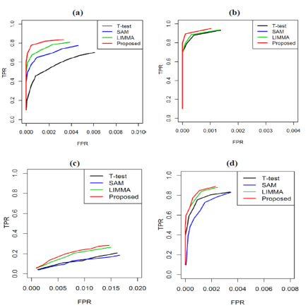
Figure 1: Performance evaluation using ROC-curve produced by the four methods (T-test, SAM, LIMMA and Proposed) based on 100 datasets with pDEG=0.02. Datasets were generated from normal distribution for (a) and (b) and datasets were generated from t-distribution for (c) and (d), where (a) and (c) represents ROC curve for small-sample case (n1=n2=3) and (b) and (d) represents ROC curve for large-sample case (n1=n2=15).

Table 1: Performance evaluation of different methods based on simulated gene expression dataset generated from normal distribution.

Methods	With proportion of DE gene (pDEG) = 0.02
	TPR	TNR	FPR	FNR	MER	FDR	AUC
T-test	0.702 (0.932)	0.006 (0.001)	0.994 (0.999)	0.298 (0.068)	0.012 (0.003)	0.298 (0.068)	0.702 (0.932)
SAM	0.775 (0.935)	0.005 (0.001)	0.995 (0.999)	0.225 (0.065)	0.009 (0.003)	0.225 (0.065)	0.775 (0.935)
LIMMA	0.810 (0.935)	0.004 (0.001)	0.996 (0.999)	0.190 (0.065)	0.008 (0.003)	0.190 (0.065)	0.810 (0.935)
Proposed	0.890 (0.935)	0.002 (0.001)	0.998 (0.999)	0.110 (0.050)	0.004 (0.002)	0.110 (0.050)	0.890 (0.950)
Methods	With proportion of DE gene (pDEG) = 0.06
	TPR	TNR	FPR	FNR	MER	FDR	AUC
T-test	0.772 (0.933)	0.012 (0.004)	0.988 (0.996)	0.228 (0.067)	0.023 (0.007)	0.228 (0.067)	0.771 (0.933)
SAM	0.810 (0.933)	0.010 (0.004)	0.990 (0.996)	0.190 (0.067)	0.019 (0.007)	0.190 (0.067)	0.809 (0.933)
IMMA	0.823 (0.933)	0.009 (0.004)	0.991 (0.996)	0.177 (0.067)	0.018 (0.007)	0.177 (0.067)	0.823 (0.933)
Proposed	0.911 (0.959)	0.005 (0.002)	0.995 (0.996)	0.089 (0.041)	0.009 (0.004)	0.089 (0.041)	0.911 (0.933)

3.3 Simulated Gene Expression Profiles generated from t- Distribution

We also investigated the performance of the proposed method in a comparison of other three methods (T-test, SAM and LIMMA) for non-normal case; accordingly we generated 100 simulated datasets from t-distribution with 10 degrees of freedom. We set the mean and variance as before. We estimated different performance measures such as TPR, TNR, FPR, FNR, MER, FDR and AUC based on 20 estimated DE genes by four methods for each of 100 datasets. The average values of performance measures are summarized in Table 2. From this table we notice that the performances of all the methods deteriorated when the datasets came from t-distribution. We also observe that the proposed method performed better than the other three methods (T-test, SAM and LIMMA). For example, the proposed method produces AUC = $0.469$ ($0.887$) which is larger than $0.316$ ($0.830$), $0.326$ ($0.832$) and $0.411$ ($0.880$) for the competitors T-test, SAM and LIMMA. The boxplots in Fig.3 and ROC curve in Fig.1(c-d) also revealed similar results like Table 2. We also noticed from boxplots that the proposed method has less variability among the other three methods. From this analysis we may conclude that the performance of the proposed method has improved than the three well-known gene selection methods.

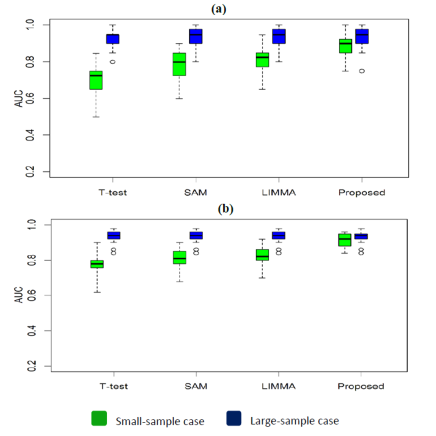
Figure 2: Performance evaluation using boxplot of AUC values produced by the four methods (T-test, SAM, LIMMA and Proposed) based on 100 datasets were taken from normal distribution for small-and large-sample cases (a) Boxplot of AUC values with proportion of DE gene=0.02. (b) Boxplot of AUC values with proportion of DE gene=0.06. Each dataset contains p =1000 genes.

Table 2: Performance evaluation of different methods based on simulated gene expression dataset generated from t-distribution

Methods	With proportion of DE gene (pDEG) = 0.02
	TPR	TNR	FPR	FNR	MER	FDR	AUC
T-test	0.318 (0.830)	0.014 (0.003)	0.986 (0.997)	0.682 (0.170)	0.027 (0.007)	0.682 (0.170)	0.316 (0.830)
SAM	0.328 (0.832)	0.014 (0.003)	0.986 (0.997)	0.672 (0.168)	0.027 (0.007)	0.672 (0.168)	0.326 (0.832)
LIMMA	0.412 (0.880)	0.012 (0.002)	0.988 (0.998)	0.588 (0.120)	0.024 (0.005)	0.588 (0.120)	0.411 (0.880)
Proposed	0.470 (0.888)	0.011 (0.002)	0.988 (0.998)	0.530 (0.112)	0.021 (0.004)	0.530 (0.112)	0.469 (0.887)

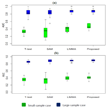
Figure 3: Performance evaluation using boxplot of AUC values produced by the four methods (T-test, SAM, LIMMA and Proposed) based on 100 datasets were taken from t-distribution distribution for small-and large-sample cases (a) Boxplot of AUC values with proportion of DE gene=0.02. (b) Boxplot of AUC values with proportion of DE gene=0.06. Each dataset contains p =1000 genes.

3.4 Application to colon cancer microarray data

The data consist of expression levels of 2000 genes obtained from a microarray study on 62 colon tissue samples collected from colon-cancer patients. Among $62$ colon tissue, $40$ tumor tissues, coded 2 and 22 normal tissues, coded 1 Alon . (1999). The goal here is to characterize the underlying interactions between genetic makers for their association with the colon-cancer patients and the healthy persons.

To calculate the influence value of each gene, we used three methods: PCAout, liner CCA and the proposed method, KCCA, respectively. Figure 4 visualizes the plots of absolute influence value for $2000$ genes. By the outliers detection technique in the one dimensional influence value of each method, we obtained $31$, $133$ and $210$ genes using PCAout, liner CCA and the proposed method KCCA, respectively. To compare the selected genes, we made a Venn-diagram of the selected genes from the three methods. Figure 5 presents the Venn-diagram of the PCOut, LCCAOut, and KCCAOut methods. From this figure, we observe that the disjoint selected genes of PCOut, LCCAOut, and KCCAOut are $19$, $61$, and $144$, respectively. The number of common genes between PCOut and LCCAOut, and PCOut and KCCAOut, and LCCAOut and KCCAOut are 7, 1, and 61, respectively. All methods selected 4 common genes: J00231, T57780, M94132 and M87789.

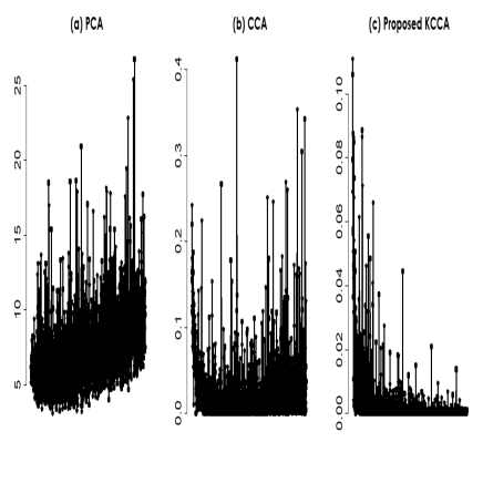
Figure 4: The influence value of genes using three methods: principal components analysis (PCOut), linear canonical correlation analysis (LCCA), and kernel canonical correlation analysis (KCCA).

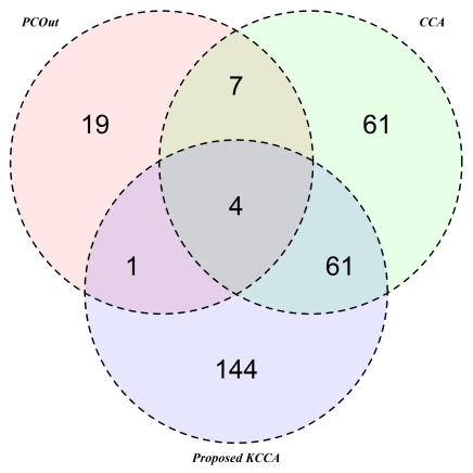
Figure 5: The Venn diagram of the selected genes using three methods: principal components analysis (PCOut), linear canonical correlation analysis (LCCA), and kernel canonical correlation analysis (KCCA).

Genes do not function alone; rather, they interact with each other. When genes share a similar set of GO annotation terms, they are most likely to be involved with similar biological mechanisms. To verify this, we extracted the gene-gene networks using STRING Szklarczyk . (2007). STRING imports protein association knowledge from databases of both physical interactions and curated biological pathways. In STRING, the simple interaction unit is the functional relationship between two proteins/genes that can contribute to a common biological purpose. Figure  6 shows the gene-gene network based on the protein interactions between the combined $210$. In this figure, the color saturation of the edges represents the confidence score of a functional association. Further network analysis shows that the number of nodes, number of edges, average node degree, clustering coefficient, PPI enrichment $p$-values are $75$, $214$, $5.71$, $0.473$ for $p\leq 8.22\times 10^{-15}$, respectively. This network of genes has significantly more interactions than expected, which indicates that they may function in a concerted effort.

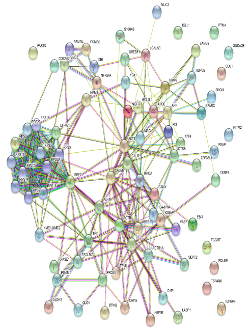
Figure 6: The network of the selected genes.

4 Concluding remarks

The kernel based methods provide more powerful and reproducible outputs, but the interpretation of the results remains challenging. Incorporating biological knowledge information (e.g., GO) can provide additional evidences on the results. The performance of the proposed method was evaluated on both simulated and a real data. The extensive simulation studies show the power gain of the proposed method relative to the alternative methods.

The utility of the proposed method is further demonstrated with the application to colon cancer microarray data. According to the influence values, the proposed method is able to rank the influence of a gene and the genes are are identified to be highly related to disease. Using a ourlier detection methods the proposed method extracts the $210$ genes out of $2000$ genes, which are considered to have significant impact on the patients. By conducting gene ontology, pathway analysis, and network analysis including visualization, we find evidences that the selected genes have a significant influence on the manifestation of colon cancer disease and can serve as a distinct feature for the classification of colon cancer patients from the healthy controls.

Although the Gaussian kernel has a free parameter (bandwidth), in this study, we used the median of the pairwise distance as the bandwidth for the Gaussian kernel, which appears to be practical. In future work, tt must be emphasized that choosing a suitable kernel is indispensable.

Acknowledgments

The authors wish to thank the University Grants Commission of Bangladesh for support.

References

- Akaho (\APACyear2001) \APACinsertmetastarAkaho{APACrefauthors}Akaho, S. \APACrefYearMonthDay2001. \BBOQ\APACrefatitleA kernel method for canonical correlation analysis A kernel method for canonical correlation analysis.\BBCQ \APACjournalVolNumPagesInternational meeting of psychometric Society.35321-377. \PrintBackRefs\CurrentBib
- Alam \BOthers. (\APACyear2016) \APACinsertmetastarAlam-2016ACMa{APACrefauthors}Alam, M\BPBIA., Calhoun, V.\BCBL \BBA Wang, Y\BHBIP. \APACrefYearMonthDay2016. \BBOQ\APACrefatitleInfluence Function of Multiple Kernel Canonical Analysis to Identify Outliers in Imaging Genetics Data Influence function of multiple kernel canonical analysis to identify outliers in imaging genetics data.\BBCQ \BIn \APACrefbtitleProceedings of the 7th ACM International Conference on Bioinformatics, Computational Biology, and Health Informatics Proceedings of the 7th acm international conference on bioinformatics, computational biology, and health informatics (\BPGS 210–219). \PrintBackRefs\CurrentBib
- Alam \BBA Fukumizu (\APACyear2013) \APACinsertmetastarAshad-13{APACrefauthors}Alam, M\BPBIA.\BCBT \BBA Fukumizu, K. \APACrefYearMonthDay2013. \BBOQ\APACrefatitleHigher-order regularized kernel CCA Higher-order regularized kernel CCA.\BBCQ \APACjournalVolNumPages12th International Conference on Machine Learning and Applications374-377. \PrintBackRefs\CurrentBib
- Alam \BBA Fukumizu (\APACyear2014) \APACinsertmetastarAshad-14{APACrefauthors}Alam, M\BPBIA.\BCBT \BBA Fukumizu, K. \APACrefYearMonthDay2014. \BBOQ\APACrefatitleHyperparameter Selection in Kernel Principal Component Analysis Hyperparameter selection in kernel principal component analysis.\BBCQ \APACjournalVolNumPagesJournal of Computer Science10(7)1139–1150. \PrintBackRefs\CurrentBib
- Alam \BBA Fukumizu (\APACyear2015) \APACinsertmetastarAshad-15{APACrefauthors}Alam, M\BPBIA.\BCBT \BBA Fukumizu, K. \APACrefYearMonthDay2015. \BBOQ\APACrefatitleHigher-Order Regularized Kernel Canonical Correlation Analysis Higher-order regularized kernel canonical correlation analysis.\BBCQ \APACjournalVolNumPagesInternational Journal of Pattern Recognition and Artificial Intelligence29(4)1551005(1-24). \PrintBackRefs\CurrentBib
- Alam \BOthers. (\APACyear2018) \APACinsertmetastarAlam-18b{APACrefauthors}Alam, M\BPBIA., Fukumizu, K.\BCBL \BBA Wang, Y\BPBIP. \APACrefYearMonthDay2018. \BBOQ\APACrefatitleInfluence function and robust variant of kernel canonical correlation analysis Influence function and robust variant of kernel canonical correlation analysis.\BBCQ \APACjournalVolNumPagesNeurocomputing30412-29. \PrintBackRefs\CurrentBib
- Alam \BOthers. (\APACyear2008) \APACinsertmetastarAshad-08{APACrefauthors}Alam, M\BPBIA., Nasser, M.\BCBL \BBA Fukumizu, K. \APACrefYearMonthDay2008. \BBOQ\APACrefatitleSensitivity analysis in robust and kernel canonical correlation analysis Sensitivity analysis in robust and kernel canonical correlation analysis.\BBCQ \APACjournalVolNumPages11th International Conference on Computer and Information Technology, Bangladesh.IEEE399-404. \PrintBackRefs\CurrentBib
- Alon \BOthers. (\APACyear1999) \APACinsertmetastarAlon-99{APACrefauthors}Alon, U., Barkai, N., Notterman, D\BPBIA., Gish, K., Ybarra, S., Mack, D.\BCBL \BBA Levine, A\BPBIJ. \APACrefYearMonthDay1999. \BBOQ\APACrefatitleBroad patterns of gene expression revealed by clustering analysis of tumor and normal colon tissues probed by oligonucleotide arrays Broad patterns of gene expression revealed by clustering analysis of tumor and normal colon tissues probed by oligonucleotide arrays.\BBCQ \APACjournalVolNumPages96(12)6745-6750. \PrintBackRefs\CurrentBib
- Alzate \BBA Suykens (\APACyear2008) \APACinsertmetastarAlzate2008{APACrefauthors}Alzate, C.\BCBT \BBA Suykens, J\BPBIA\BPBIK. \APACrefYearMonthDay2008. \BBOQ\APACrefatitleA regularized kernel CCA contrast function for ICA A regularized kernel CCA contrast function for ICA.\BBCQ \APACjournalVolNumPagesNeural Networks21170-181. \PrintBackRefs\CurrentBib
- Aronszajn (\APACyear1950) \APACinsertmetastarAron-RKHS{APACrefauthors}Aronszajn, N. \APACrefYearMonthDay1950. \BBOQ\APACrefatitleTheory of reproducing kernels Theory of reproducing kernels.\BBCQ \APACjournalVolNumPagesTransactions of the American Mathematical Society68337-404. \PrintBackRefs\CurrentBib
- Bach \BBA Jordan (\APACyear2002) \APACinsertmetastarBack-02{APACrefauthors}Bach, F\BPBIR.\BCBT \BBA Jordan, M\BPBII. \APACrefYearMonthDay2002. \BBOQ\APACrefatitleKernel independent component analysis Kernel independent component analysis.\BBCQ \APACjournalVolNumPagesJournal of Machine Learning Research31-48. \PrintBackRefs\CurrentBib
- Castellanos-Garzón \BBA Romos (\APACyear\bibnodate) \APACinsertmetastarCastellanos-15{APACrefauthors}Castellanos-Garzón, J.\BCBT \BBA Romos, J. \APACrefYearMonthDay\bibnodate. \PrintBackRefs\CurrentBib
- Charpiat \BOthers. (\APACyear\bibnodate) \APACinsertmetastarCharpiat-15{APACrefauthors}Charpiat, G., Hofmann, M.\BCBL \BBA Schölkopf, B. \APACrefYearMonthDay\bibnodate. \BBOQ\APACrefatitleKernel methods in medical imaging Kernel methods in medical imaging.\BBCQ \BIn \APACrefbtitleHandbook of Biomedical Imaging Handbook of biomedical imaging (\BPG 63-81). \APACaddressPublisherBerlin, GermanySpringer. \PrintBackRefs\CurrentBib
- Chen \BBA Ishwaran (\APACyear2012) \APACinsertmetastarXChen-12{APACrefauthors}Chen, X.\BCBT \BBA Ishwaran, H. \APACrefYearMonthDay2012. \BBOQ\APACrefatitleRandom forests for genomic data analysis Random forests for genomic data analysis.\BBCQ \APACjournalVolNumPagesGenomics99323-329. \PrintBackRefs\CurrentBib
- Debruyne \BOthers. (\APACyear2010) \APACinsertmetastarDebruyne-10{APACrefauthors}Debruyne, M., Hubert, M.\BCBL \BBA Horebeek, J. \APACrefYearMonthDay2010. \BBOQ\APACrefatitleDetecting influential observations in Kernel PCA Detecting influential observations in kernel pca.\BBCQ \APACjournalVolNumPagesComputational Statistics and Data Analysis543007-3019. \PrintBackRefs\CurrentBib
- Filzmoser \BOthers. (\APACyear2008) \APACinsertmetastarFilzmoser-08{APACrefauthors}Filzmoser, P., Maronna, R.\BCBL \BBA Werner, M. \APACrefYearMonthDay2008. \BBOQ\APACrefatitleOutlier identification in high dimensions Outlier identification in high dimensions.\BBCQ \APACjournalVolNumPagescomputational Stastistics& Data Analysis521694-1711. \PrintBackRefs\CurrentBib
- Hastie \BOthers. (\APACyear\bibnodate) \APACinsertmetastarHastei-00{APACrefauthors}Hastie, T., Tibshirani, R., Eisen, M\BPBIB., Alizadeh, A., Levy, R., Staudt, L.\BDBLP. Brown, t\BPBI. \APACrefYearMonthDay\bibnodate. \PrintBackRefs\CurrentBib
- Hofmann \BOthers. (\APACyear2008) \APACinsertmetastarHofmann-08{APACrefauthors}Hofmann, T., Schölkopf, B.\BCBL \BBA Smola, J\BPBIA. \APACrefYearMonthDay2008. \BBOQ\APACrefatitleKernel Methods in Machine Learning Kernel methods in machine learning.\BBCQ \APACjournalVolNumPagesThe Annals of Statistics361171-1220. \PrintBackRefs\CurrentBib
- Huang \BOthers. (\APACyear2009) \APACinsertmetastarHuang-2009{APACrefauthors}Huang, S\BPBIY., Lee, M.\BCBL \BBA Hsiao, C. \APACrefYearMonthDay2009. \BBOQ\APACrefatitleNonlinear measures of association with kernel canonical correlation analysis and applications Nonlinear measures of association with kernel canonical correlation analysis and applications.\BBCQ \APACjournalVolNumPagesJournal of Statistical Planning and Inference1392162-2174. \PrintBackRefs\CurrentBib
- Richfield \BOthers. (\APACyear2017) \APACinsertmetastarRichfield-17{APACrefauthors}Richfield, O., Alam, M\BPBIA., Calhoun, V.\BCBL \BBA Wang, Y\BPBIP. \APACrefYearMonthDay2017. \BBOQ\APACrefatitleLearning Schizophrenia Imaging Genetics Data Via Multiple Kernel Canonical Correlation Analysis Learning schizophrenia imaging genetics data via multiple kernel canonical correlation analysis.\BBCQ \APACjournalVolNumPagesProceedings - 2016 IEEE International Conference on Bioinformatics and Biomedicine, BIBM 2016, Shenzhen, China5507-5011. \PrintBackRefs\CurrentBib
- Romanazzi (\APACyear1992) \APACinsertmetastarRomanazii-92{APACrefauthors}Romanazzi, M. \APACrefYearMonthDay1992. \BBOQ\APACrefatitleInfluence in Canonical Correlation Analysis Influence in canonical correlation analysis.\BBCQ \APACjournalVolNumPagesPsychometrika57(2)237-259. \PrintBackRefs\CurrentBib
- Ruan \BBA Yuan (\APACyear2011) \APACinsertmetastarRuan-11{APACrefauthors}Ruan, L.\BCBT \BBA Yuan, M. \APACrefYearMonthDay2011. \BBOQ\APACrefatitleAn Empirical Bayes’ Approach to Joint Analysis of Multiple Microarray Gene Expression Studies An empirical bayes’ approach to joint analysis of multiple microarray gene expression studies.\BBCQ \APACjournalVolNumPagesBiometrics671617-1626. \PrintBackRefs\CurrentBib
- Szklarczyk \BOthers. (\APACyear2007) \APACinsertmetastarSTRING-15{APACrefauthors}Szklarczyk, D., Franceschini, A., Wyder, S., Forslund, K., Heller, D., Huerta-Cepas, J.\BDBLvon Mering, C. \APACrefYearMonthDay2007. \BBOQ\APACrefatitleSTRING v10: Protein-protein Interaction Networks, Integrated over the Tree of Life STRING v10: Protein-protein interaction networks, integrated over the tree of life.\BBCQ \APACjournalVolNumPagesNucleic Acids Research43531–543. \PrintBackRefs\CurrentBib
- Tanaka (\APACyear1988) \APACinsertmetastarTanaka-88{APACrefauthors}Tanaka, Y. \APACrefYearMonthDay1988. \BBOQ\APACrefatitleSensitivity analysis in principal component analysis: influence on the subspace spanned by principal components Sensitivity analysis in principal component analysis: influence on the subspace spanned by principal components.\BBCQ \APACjournalVolNumPagesCommunications in Statistics-Theory and Methods17(9)3157–3175. \PrintBackRefs\CurrentBib
- Tanaka (\APACyear1989) \APACinsertmetastarTanaka-89{APACrefauthors}Tanaka, Y. \APACrefYearMonthDay1989. \BBOQ\APACrefatitleInfluence functions related to eigenvalue problem which appear in multivariate analysis Influence functions related to eigenvalue problem which appear in multivariate analysis.\BBCQ \APACjournalVolNumPagesCommunications in Statistics-Theory and Methods18(11)3991–4010. \PrintBackRefs\CurrentBib