Nonlinear gap modes and compactons in a lattice model for spin-orbit coupled exciton-polaritons in zigzag chains

Abstract

We consider a system of generalized coupled Discrete Nonlinear Schrödinger (DNLS) equations, derived as a tight-binding model from the Gross-Pitaevskii-type equations describing a zigzag chain of weakly coupled condensates of exciton-polaritons with spin-orbit (TE-TM) coupling. We focus on the simplest case when the angles for the links in the zigzag chain are $\pm\pi/4$ with respect to the chain axis, and the basis (Wannier) functions are cylindrically symmetric (zero orbital angular momenta). We analyze the properties of the fundamental nonlinear localized solutions, with particular interest in the discrete gap solitons appearing due to the simultaneous presence of spin-orbit coupling and zigzag geometry, opening a gap in the linear dispersion relation. In particular, their linear stability is analyzed. We also find that the linear dispersion relation becomes exactly flat at particular parameter values, and obtain corresponding compact solutions localized on two neighboring sites, with spin-up and spin-down parts $\pi/2$ out of phase at each site. The continuation of these compact modes into exponentially decaying gap modes for generic parameter values is studied numerically, and regions of stability are found to exist in the lower or upper half of the gap, depending on the type of gap modes.

I Introduction

Planar semiconductor microcavities operating in the exciton-polariton regime have become a paradigm model for experimental and theoretical studies of nonlinear and quantum properties of light-matter interaction ds1 . A major advantage of these systems is that they are solid state devices, that operate in a wide diapason of temperatures between few Kelvins and up to the room conditions. Interaction between the polaritons is much stronger than for pure photons, that lowers power requirements for creating conditions when polariton dynamics can be effectively controlled with the external light sources ds2 . Microcavities can also be readily structured to create a variety of potential energy landscapes reproducing lattice structures known in studies of electrons in condensed matter on more practical scales of tens of microns. Thus polaritons can be controlled using band gap and zone engineering ds3 . Through their peculiar spin properties and sensitivity to the applied magnetic field, polaritons in structured microcavities have been shown to have a number of topological properties ds4 . Thus polariton based devices have a competitive edge over their photon-only counterparts through their relatively low nonlinear thresholds and possibility to create micron-scale topological devices. A combination of these two aspects has been recently used to demonstrate a variety of nonlinear topological effects in polariton systems, see, e.g., ds5 and references therein.

As a specific example, a polariton BEC in a zigzag chain of polariton micropillars with photonic spin-orbit coupling, originating in the splitting of optical cavity modes with TE and TM polarization, was proposed in Ref. Solnyshkov16 . The simultaneous presence of zigzag geometry and polarization dependent tunneling was shown to yield topologically protected edge states, and in the presence of homogeneous pumping and nonlinear interactions the creation of polarization domain walls through the Kibble-Zurek mechanism, analogous to the Su-Schrieffer-Heeger solitons in polymers, was numerically observed Solnyshkov16 . Of crucial importance is the spin-orbit induced opening of a central gap in the linear dispersion relation. As we will show in this work, the existence of a gap, together with the option of tuning the linear dispersion towards flatness at specific parameter values, also leads to nonlinear strongly localized modes in the bulk (intrinsically localized modes) with properties depending crucially on the relative strength of interaction between polaritons of opposite and equal spin.

The starting point is the following set of two coupled continuous Gross-Pitaevskii equations Flayac10 :

$$i\partial_{t}{\Psi}_{+}=-\frac{1}{2}(\partial_{x}^{2}+\partial_{y}^{2})\Psi_{+}+\left(|\Psi_{+}|^{2}+\mathfrak{a}|\Psi_{-}|^{2}\right)\Psi_{+}+\Omega\Psi_{+}+\beta(\partial_{x}-i\partial_{y})^{2}\Psi_{-}+V(x,y){\Psi}_{+}$$

$$i\partial_{t}{\Psi}_{-}=-\frac{1}{2}(\partial_{x}^{2}+\partial_{y}^{2})\Psi_{-}+\left(|\Psi_{-}|^{2}+\mathfrak{a}|\Psi_{+}|^{2}\right)\Psi_{-}-\Omega\Psi_{-}+\beta(\partial_{x}+i\partial_{y})^{2}\Psi_{+}+V(x,y){\Psi}_{-}.$$ (1)

These equations describe exciton-polaritons with circularly polarized light-component, where $\Psi_{+}$ corresponds to left (positive spin) and $\Psi_{-}$ to right (negative spin) polarization. Polaritons interact mainly through their excitonic part, and interactions between polaritons with identical polarization are generally repulsive (here normalized to +1), while interactions between those of opposite spins often are weaker and attractive. A typical value is $\mathfrak{a}\simeq-0.05$ Sich14 , but may range between roughly $-1\lesssim\mathfrak{a}\lesssim 0$, and may possibly be also repulsive, or attractive with a magnitude stronger than the self-interaction Vladimirova10 . Since the exciton-components of the polariton wave functions typically are localized within small spatial regions, the interactions are assumed to be local (point interactions) in this mean-field description. $\Omega$ describes the Zeeman-splitting between spin-up and spin-down polaritons in presence of an external magnetic field; in this work we put $\Omega=0$.

Of main interest here is the term proportional to $\beta$: it arises due to different properties associated with polaritons whose photonic components, as expressed in a suitable basis of linear polarization, have TE resp TM polarizations (or, alternatively, longitudinal/transversal w.r.t. the propagation direction (${\bf k}$-vector)). It is commonly described in terms of different effective masses of the lower polariton branches for TE and TM components, $\beta\propto m_{TE}^{-1}-m_{TM}^{-1}$, whose ratio typically may be of the order $m_{TE}/m_{TM}\approx 0.85-0.95$ (see e.g. supplemental material of Dufferwiel15 ), although in principle $\beta$ could have arbitrary sign. Expressed in a basis of circular polarization (spinor basis) as in (1) ($\Psi_{\pm}=\Psi_{x}\mp i\Psi_{y}$), this TE/TM energy splitting can be interpreted as a spin-orbit splitting, since the dynamics of the two spin (polarization) components couple in a different way to the orbital part of the other component (via derivatives in $x$ and $y$ of the mean-field wave function in (1)).

In this work, we choose the potential $V(x,y)$ as a zigzag potential along the $x$-direction, considering this geometry as the simplest generalization of a straight 1D chain which yields non-trivial geometrical effects of the spin-orbit coupling between polaritons localized at neighboring potential minima. As an example potential, we may choose e.g.:

$$V(x,y)=-2V_{0}\sin\left(\frac{\sqrt{2}\pi}{d}x\right)\sin{\left(\frac{\sqrt{2}\pi}{d}y\right)};\quad 0\leq x\leq N\sqrt{2}d,\ 0\leq y\leq\sqrt{2}d,$$ (2)

as illustrated in Fig. 1. Here $d$ is the distance between potential mininma, and $2N$ is the total number of potential wells in the chain. The geometry is essentially the same as for the coupled micropillars in Solnyshkov16 , with all angles for the links between neighboring minima being $\pm 45^{\circ}$ with respect to the $x$-axis. Evidently one may easily generalize to arbitrary angles, or more complicated expressions for zigzag potentials which may be realized in various experimental settings e.g. with optical lattices Zhang15 . In order to motivate a tight-binding approximation, we assume $V_{0}\gg 1$.

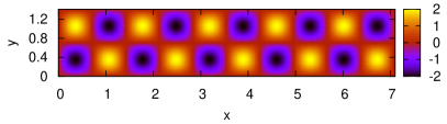
Figure 1: The zigzag potential $V(x,y)$ (2) with $V_{0}=d=1$ and $N=5$. In the tight-binding expansion (3), the Wannier functions are assumed to be centered around the lattice minima.

In order to understand the most important effects of the spin-coupling coupling in (1) in a tight-binding framework, we here consider situations where the effects of spin-orbit splitting inside each potential well can be neglected, and only are relevant in the regions of wavefunction overlap between neighboring wells. For the experimental set-up of Dufferwiel15 , this should be a good approximation if the spatial modes inside the wells may be approximated with Laguerre-Gauss modes with zero orbital angular momentum ($LG_{00}^{\pm}$ in the notation of Dufferwiel15 , where the two subscripts stand for radial and orbital quantum numbers of the 2D harmonic-oscillator wave function, and the superscript indicates polarization as in (1).) At least for a single cavity of non-interacting polaritons, these modes should be good approximations to the ground state, so let us assume that interactions (nonlinearity) and spin-orbit couplings are sufficiently weak to be treated perturbatively, along with the inter-well overlaps. The approach may be extended to consider also lattices of spin vortices (excited modes) built up from modes with nonzero OAM (e.g. $LG_{0\pm 1}^{\pm}$ as considered in Dufferwiel15 ); however this will introduce some additional complications and will be left for future work.

Moreover, if $V_{0}\gg 1$ we may also neglect the effect of next-nearest-neighbor interactions (distances between two wells in the horizontal $x$-direction is $\sqrt{2}$ times larger than between nearest neighbors). It may then be a good approximation to use, as the basis set for the tight-binding approximation, the Wannier functions for a full 2D square lattice (these issues are discussed and numerically checked for some realization of a zigzag optical lattice in a recent Master thesis Gagge16 ). These may resemble (but certainly differ from) Gagge16 the LG individual modes (e.g. Wannier functions typically have radial oscillatory tails, decaying exponentially rather than Gaussian). In any case, we will assume that the basis functions $w(x,y)$ (expressed in Cartesian coordinates) are qualitatively close to the $LG_{00}$ modes. Particularly, they will be assumed to be close to cylindrically symmetric ($w(x,y)\sim e^{-\omega(x^{2}+y^{2})}$ in the harmonic approximation). (Note that this assumption would not be valid for spin vortices arising from LG modes with nonzero OAM.)

The outline of this paper is as follows. In Sec. II we derive the tight-binding model, discuss its general properties, and illustrate the linear dispersion relation for the case with $\pm 45^{\circ}$ angles which will be the system studied for the rest of this paper. We also in Sec. II.5 identify a limit where the linear dispersion relation becomes exactly flat, and identify the corresponding fundamental compact solutions. In Sec. III we construct the fundamental nonlinear localized modes in the semi-infinite gaps above or below the linear spectrum, as well as in the mini-gap between the linear dispersion branches, opened up due to the simultaneous presence of spin-orbit coupling and nontrivial geometry. Analytical calculations using perturbation theory from the weak-coupling and flat-band limits for the semi-infinite and mini-gap, respectively, are compared with numerical calculations using a standard Newton scheme. In Sec. IV the linear stability of the different families of nonlinear localized modes is investigated, and some instability scenarios are illustrated with direct dynamical simulations. Finally, some concluding remarks are given in Sec. V.

II Model

II.1 Derivation of the tight-binding model

Under the above assumptions, we may expand:

$$\Psi_{+}=\sum_{n=1}^{2N}u_{n}(t)w(x^{\prime}-nd^{\prime},y^{\prime}-(-1)^{n}d^{\prime}/2),\quad\Psi_{-}=\sum_{n=1}^{2N}v_{n}(t)w(x^{\prime}-nd^{\prime},y^{\prime}-(-1)^{n}d^{\prime}/2),$$ (3)

where, relative to the coordinate system of (2) and Fig. 1, $d^{\prime}=d/\sqrt{2},x^{\prime}=x-d^{\prime}/2,y^{\prime}=y-d^{\prime}$. Note that the (Wannier) basis functions are the same for both components, since we have assumed no spin-orbit splitting inside the wells, $\Omega=0$, and $w$ are basis functions of the linear problem. Note also that an analogous approach was used in Salerno15 to derive lattice equations for the simpler problem of a pure 1D lattice with a standard spin-orbit coupling term ($-i\partial_{x}$, linear in the spatial derivative) for atomic BEC’s in optical lattices; similar models were also studied in Sakaguchi14 ; Belicev15 ; Gligoric16 . For simplicity we will assume below that $w(x,y)$ can be chosen real (which is typically the case in absence of OAM; the generalization to modes with nonzero OAM requires complex $w(x,y)$ and will be treated in a separate work).

Inserting the expansion (3) into (1), we obtain for the first component:

$$i\sum_{n^{\prime}}\dot{u}_{n^{\prime}}w(x^{\prime}-n^{\prime}d^{\prime},y^{\prime}-(-1)^{n^{\prime}}d^{\prime}/2)$$

$$=-\frac{1}{2}\sum_{n^{\prime}}{u}_{n^{\prime}}\left[w_{xx}(x^{\prime}-n^{\prime}d^{\prime},y^{\prime}-(-1)^{n^{\prime}}d^{\prime}/2)+w_{yy}(x^{\prime}-n^{\prime}d^{\prime},y^{\prime}-(-1)^{n^{\prime}}d^{\prime}/2)\right]$$

$$+\sum_{n^{\prime}}\left(|u_{n^{\prime}}|^{2}+\mathfrak{a}|v_{n^{\prime}}|^{2}\right)u_{n^{\prime}}w^{3}(x^{\prime}-n^{\prime}d^{\prime},y^{\prime}-(-1)^{n^{\prime}}d^{\prime}/2)$$

$$+\beta\sum_{n^{\prime}}{v}_{n^{\prime}}\left[w_{xx}(x^{\prime}-n^{\prime}d^{\prime},y^{\prime}-(-1)^{n^{\prime}}d^{\prime}/2)-w_{yy}(x^{\prime}-n^{\prime}d^{\prime},y^{\prime}-(-1)^{n^{\prime}}d^{\prime}/2)-2iw_{xy}(x^{\prime}-n^{\prime}d^{\prime},y^{\prime}-(-1)^{n^{\prime}}d^{\prime}/2\right]$$

$$+V(x,y)\sum_{n^{\prime}}{u}_{n^{\prime}}w(x^{\prime}-n^{\prime}d^{\prime},y^{\prime}-(-1)^{n^{\prime}}d^{\prime}/2).$$ (4)

Here, in writing the nonlinear term as a simple sum and not a triple, we have neglected overlap between basis functions on different sites in cubic terms in $w$ (assuming strong localization of $w$).

Multiplying with $w^{(n)}\equiv w(x^{\prime}-nd^{\prime},y^{\prime}-(-1)^{n}d^{\prime}/2)$, integrating over $x$ and $y$, using the orthogonality of Wannier functions and neglecting all overlaps beyond nearest neighbors, we obtain from (4) a 1D lattice equation of the following form for the site amplitudes of the spin-up component:

$$i\dot{u}_{n}=\epsilon u_{n}-\Gamma\left(u_{n+1}+u_{n-1}\right)+\gamma\left(|u_{n}|^{2}+\mathfrak{a}|v_{n}|^{2}\right)u_{n}+\omega v_{n}+\sigma_{n,n+1}v_{n+1}+\sigma_{n,n-1}v_{n-1}.$$ (5)

Here the coefficients are: On-site energy,

$$\epsilon=\int\int\left[-\frac{1}{2}(w^{(n)}_{xx}+w^{(n)}_{yy})+V(x,y)w^{(n)}\right]w^{(n)}dxdy;$$

linear coupling coefficients,

$$\Gamma=\frac{1}{2}\int\int(w^{(n+1)}_{xx}+w^{(n+1)}_{yy})w^{(n)}dxdy=\frac{1}{2}\int\int(w^{(n-1)}_{xx}+w^{(n-1)}_{yy})w^{(n)}dxdy,$$

where the second equality is obviously true if $w^{(n)}$ is cylindrically symmetric; nonlinearity coefficient,

$$\gamma=\int\int(w^{(n)})^{4}dxdy;$$

on-site spin-orbit interaction,

$$\omega=\beta\int\int(w^{(n)}_{xx}-w^{(n)}_{yy}-2iw^{(n)}_{xy})w^{(n)}dxdy,$$

which is identically zero if $w^{(n)}$ is cylindrically symmetric (easiest seen in polar coordinates, with $w=w(r)$ only, $\omega=\beta\int_{0}^{2\pi}d\phi e^{-2i\phi}\int rdr(w_{rr}-\frac{w_{r}}{r})w=0$) (but generally nonzero if Wannier modes would have OAM); and nearest-neighbor spin-orbit interactions (the relevant ’new’ terms here),

$$\sigma_{n,n\pm 1}=\beta\int\int(w^{(n\pm 1)}_{xx}-w^{(n\pm 1)}_{yy}-2iw^{(n\pm 1)}_{xy})w^{(n)}dxdy.$$ (6)

Since tails of $w$ are exponentially small, we may assume all integrals taken over the infinite plane. Explicitly, with a change of origin we may write e.g. the first term in the integral in (6) as $\int\int w_{xx}(x\mp d^{\prime},y-(-1)^{n}d^{\prime})w(x,y)dxdy$, etc. But for the case with $w$ cylindrically symmetric, we may easier evaluate the integral (6) in polar coordinates, centered at site $n\pm 1$. After some elementary trigonometry we then obtain:

$$\sigma_{n,n\pm 1}=\beta\int\int e^{-i2\phi}\left(w_{rr}-\frac{w_{r}}{r}\right)w(\sqrt{d^{2}+r^{2}\pm 2dr\cos\left(\frac{\pi}{4}\pm(-1)^{n}\phi\right)})rdrd\phi.$$ (7)

Letting $\phi^{\prime}=\frac{\pi}{4}\pm(-1)^{n}\phi$, this can be expressed as

$$\sigma_{n,n\pm 1}=e^{\pm 2i\alpha_{n}}\sigma;\quad\sigma\equiv\beta\int\int e^{\mp(-1)^{n}i2\phi^{\prime}}\left(w_{rr}-\frac{w_{r}}{r}\right)w(\sqrt{d^{2}+r^{2}\pm 2dr\cos\phi^{\prime}})rdrd\phi^{\prime},$$ (8)

where $\alpha_{n}\equiv(-1)^{n}\frac{\pi}{4}$ are the angles for the links in the zigzag chain with respect to the $x$-axis, and the integral defining $\sigma$ is independent of all signs since $\cos\phi^{\prime}$ is even. Explicitly, for the $\pi/4$ zigzag chain we get

$$\sigma_{n,n\pm 1}=\left\{\begin{array}[]{rl}-i\sigma&\text{diagonal links}\\ +i\sigma&\text{antidiagonal links}\end{array}\right..$$ (9)

Proceeding analogously with the second component, we obtain the corresponding lattice equation for the site-amplitudes of the spin-down component:

$$i\dot{v}_{n}=\epsilon v_{n}-\Gamma\left(v_{n+1}+v_{n-1}\right)+\gamma\left(|v_{n}|^{2}+\mathfrak{a}|u_{n}|^{2}\right)v_{n}+\omega^{\prime}u_{n}+\sigma^{\prime}_{n,n+1}u_{n+1}+\sigma^{\prime}_{n,n-1}u_{n-1}.$$ (10)

Here, $\epsilon,\Gamma,\gamma$ are identical as for the first component (i.e., we may put $\epsilon=0$ by redefining zero-energy, and $\gamma=1$ (or alternatively $\Gamma=1$) by redefining energy scale). For the on-site spin-orbit interaction,

$$\omega^{\prime}=\beta\int\int(w^{(n)}_{xx}-w^{(n)}_{yy}+2iw^{(n)}_{xy})w^{(n)}dxdy,$$

(note opposite sign of third term compared to $\omega$), which is again zero if $w$ is cylindrically symmetric. And finally, for the nearest-neighbor spin-orbit couplings,

$$\sigma^{\prime}_{n,n\pm 1}=\beta\int\int(w^{(n\pm 1)}_{xx}-w^{(n\pm 1)}_{yy}+2iw^{(n\pm 1)}_{xy})w^{(n)}dxdy$$ (11)

(again note sign of third term compared to (6). As before, restricting to cylindrically symmetric $w$ yields

$$\sigma^{\prime}_{n,n\pm 1}=\beta\int\int e^{+i2\phi}\left(w_{rr}-\frac{w_{r}}{r}\right)w(\sqrt{d^{2}+r^{2}\pm 2dr\cos\left(\frac{\pi}{4}\pm(-1)^{n}\phi\right)})rdrd\phi$$

$$=\beta e^{\mp(-1)^{n}i\pi/2}\int\int e^{\pm(-1)^{n}i2\phi^{\prime}}\left(w_{rr}-\frac{w_{r}}{r}\right)w(\sqrt{d^{2}+r^{2}\pm 2dr\cos\phi^{\prime}})rdrd\phi^{\prime}=e^{\mp 2i\alpha_{n}}\sigma,$$ (12)

where the last equality holds since the integral is equivalent to that of (8). Explicitly, for the $\pi/4$ zigzag chain

$$\sigma^{\prime}_{n,n\pm 1}=\left\{\begin{array}[]{rl}+i\sigma&\text{diagonal links}\\ -i\sigma&\text{antidiagonal links}\end{array}\right.,$$ (13)

i.e., with opposite signs compared to (9). Note that, under the above assumptions ($w$ real and cylindrically symmetric), the integral defining $\sigma$ is always real.

We note that the resulting lattice equations (5), (10), with spin-orbit coefficients given by (9), (13), are not equivalent to the equations studied in Salerno15 ; Belicev15 ; Sakaguchi14 ; Gligoric16 . In particular, we comment on the relation between the present model and that of Ref. Gligoric16 , who considered a diamond chain with angles $\pi/4$ and a Rashba-type spin-orbit coupling. The zigzag chain could be considered as e.g. the upper part of the diamond chain, if all amplitudes of the lower strand would vanish. However, because the spin-orbit coupling used in Gligoric16 is linear in the spatial derivatives while in this work it is quadratic, the spin-orbit coupling coefficients in Gligoric16 have a phase shift of $\pi/2$ between diagonal and antidiagonal links, compared to $\pi$ in (9), (13).

II.2 General properties of the TB-equations

Let us put $\epsilon=0$ and $\gamma=1$. As above, assuming cylindrically symmetric basis functions, we have $\omega=\omega^{\prime}=0$. We also remind the reader that we consider the case with no external magnetic field, $\Omega=0$ in (1). Equations (5) and (10), with spin-orbit coefficients given by (9) and (13), respectively, then become:

$$i\dot{u}_{n}=-\Gamma\left(u_{n+1}+u_{n-1}\right)+\left(|u_{n}|^{2}+\mathfrak{a}|v_{n}|^{2}\right)u_{n}+(-1)^{n}i\sigma\left(v_{n+1}-v_{n-1}\right)\quad\text{(spin-up)};$$

$$i\dot{v}_{n}=-\Gamma\left(v_{n+1}+v_{n-1}\right)+\left(|v_{n}|^{2}+\mathfrak{a}|u_{n}|^{2}\right)v_{n}-(-1)^{n}i\sigma\left(u_{n+1}-u_{n-1}\right)\quad\text{(spin-down)}.$$ (14)

One may easily show the existence of the “standard” two conserved quantities for DNLS-type models; Norm (Power):

$$P=\sum_{n}\left(|u_{n}|^{2}+|v_{n}|^{2}\right),$$ (15)

and Hamiltonian:

$$H=\sum_{n}\left\{-\Gamma\left(u_{n}^{*}u_{n+1}+v_{n}^{*}v_{n+1}\right)+\frac{1}{4}\left(|u_{n}|^{4}+|v_{n}|^{4}\right)+\frac{\mathfrak{a}}{2}|u_{n}|^{2}|v_{n}|^{2}+(-1)^{n}i\sigma u_{n}^{*}\left(v_{n+1}-v_{n-1}\right)\right\}+c.c..$$ (16)

Here, $\{u_{n},v_{n}\}$ and $\{iu^{*}_{n},iv^{*}_{n}\}$ play the role of conjugated coordinates and momenta, respectively (i.e., $\dot{u}_{n}=\partial H/\partial(iu^{*}_{n}),\dot{v}_{n}=\partial H/\partial(iv^{*}_{n})$, etc.). We may note that the Hamiltonian is similar to the Hamiltonian for the “inter-SOC” chain of Beličev et al. (Eq. (11) in Belicev15 ), but differs by the “zigzag” spin-orbit factor $(-1)^{n}$ in the last term. Note that this factor can be removed by performing a “staggering transformation” on the site-amplitudes of the spin-down component: $v_{n}^{\prime}=(-1)^{n}v_{n}$, transforming the equations of motion (14) into:

$$i\dot{u}_{n}=-\Gamma\left(u_{n+1}+u_{n-1}\right)+\left(|u_{n}|^{2}+\mathfrak{a}|v_{n}^{\prime}|^{2}\right)u_{n}-i\sigma\left(v_{n+1}^{\prime}-v_{n-1}^{\prime}\right)\quad\text{(spin-up)};$$

$$i\dot{v}_{n}^{\prime}=+\Gamma\left(v_{n+1}^{\prime}+v_{n-1}^{\prime}\right)+\left(|v_{n}^{\prime}|^{2}+\mathfrak{a}|u_{n}|^{2}\right)v_{n}^{\prime}-i\sigma\left(u_{n+1}-u_{n-1}\right)\quad\text{(spin-down)}.$$ (17)

Thus, this transformation effectively changes the sign of the linear coupling of the spin-down component into $\Gamma\rightarrow\Gamma^{\prime}=-\Gamma$ (which may be interpreted as a reversal of the “effective mass” of the spin-down polariton in this tight-binding approximation), while the nonlinear and spin-orbit terms for both components become equivalent. Eqs. (17) differ from the equations derived in Salerno15 for the straight chain with standard spin-orbit coupling only through this sign-change of $\Gamma$ for the spin-down component. Note also that Eqs. (17) are invariant under a transformation $v_{n}^{\prime}\rightarrow-v_{n}^{\prime}$, $n+1\rightarrow n-1$, i.e., an overall change of the relative sign of the spin-up and spin-down components is equivalent to a spatial inversion.

II.3 Generalization to arbitrary angles

As mentioned, it is straightforward to generalize the derivation of the tight-binding equations to arbitrary bonding angles $\alpha\neq\pi/4$ in the zigzag chain. We just outline the main steps: In (3) and the following, we replace $y^{\prime}-(-1)^{n}d^{\prime}/2$ with $y^{\prime}-(-1)^{n}\tan(\alpha)d^{\prime}/2$ (having redefined $d^{\prime}=d\cos\alpha$). In (7), (12), $\pi/4$ then get replaced by $\alpha$, as already indicated. In (9) we get $e^{-i2\alpha}\sigma$ for diagonal links and $e^{i2\alpha}\sigma$ for antidiagonal, and in (13) we get $e^{i2\alpha}\sigma$ for diagonal links and $e^{-i2\alpha}\sigma$ for antidiagonal. Then in the tight-binding equations of motion (14), the last term for the spin-up component gets replaced by $+e^{(-1)^{n}i2\alpha}v_{n+1}-e^{-(-1)^{n}i2\alpha}v_{n-1}$, and for the spin-down component by $+e^{-(-1)^{n}i2\alpha}u_{n+1}-e^{(-1)^{n}i2\alpha}u_{n-1}$. For the rest of this paper we will assume $\alpha=\pi/4$ and leave the study of effects of variation of the binding angle to future work.

II.4 Linear dispersion relation

Figure 2: The dispersion relation (18) with $\Gamma=1$ and $\sigma=0.1$.

Let $u_{n}=ue^{i(kn-\mu t)},v_{n}=ve^{i[(k+\pi)n-\mu t]}$ (i.e., $v_{n}^{\prime}=ve^{i(kn-\mu t)}$ removing factors $(-1)^{n}$), with $|u|,|v|\ll 1$. Inserting it into (14) (or (17)) and neglecting the nonlinear terms then yields:

$$\mu_{1,2}(k)=\pm 2\sqrt{\Gamma^{2}\cos^{2}k+\sigma^{2}\sin^{2}k}.$$ (18)

Thus, as illustrated in Fig. 2 (assuming $\sigma<\Gamma$), the spin-orbit coupling opens up gaps in the linear dispersion relation at $k=\pm\pi/2$, of width $4\sigma$. Note that in contrast to the models for straight chains studied in Belicev15 ; Salerno15 , no external magnetic field is needed to open the gap for the zigzag chain. The gap opening is a consequence of the simultaneous presence of spin-orbit coupling and nontrivial geometry, which was also noted for the more complicated diamond chain in Gligoric16 .

The amplitude ratios between the components may be obtained as $v/u=\frac{-\Gamma\cos k\mp\sqrt{\Gamma^{2}\cos^{2}k+\sigma^{2}\sin^{2}k}}{\sigma\sin k}$. For weak spin-orbit coupling ($\sigma\ll\Gamma$), the polariton is mainly spin-up ($u\gg v$) on the lower dispersion branch and spin-down on the upper branch ($v\gg u$) when $\Gamma\cos k>0$, and the opposite when $\Gamma\cos k<0$.

II.5 Flat band and compact modes

We may also note that in the particular case of $|\Gamma|=|\sigma|$, the dispersion relation becomes exactly flat. In this case, there are eigenmodes completely localized on either upper or lower part of the chain, with alternating $v_{n}=\pm iu_{n}$ on this part (i.e., $v_{n}\equiv u_{n}\equiv 0$ either for odd or even $n$). These modes persist also in the presence of nonlinearity (interactions). With the flat band, it is also possible to construct exact compact solutions localized on two neighboring sites. Explicitly, we get for $\sigma=+\Gamma$:

$$\left(\begin{array}[]{c}u_{n_{0}}\\ v_{n_{0}}^{\prime}\end{array}\right)=Ae^{-i\mu t}\left(\begin{array}[]{c}1\\ i\end{array}\right);\left(\begin{array}[]{c}u_{n_{0}+1}\\ v_{n_{0}+1}^{\prime}\end{array}\right)=\pm Ae^{-i\mu t}\left(\begin{array}[]{c}1\\ -i\end{array}\right),$$ (19)

and for $\sigma=-\Gamma$:

$$\left(\begin{array}[]{c}u_{n_{0}}\\ v_{n_{0}}^{\prime}\end{array}\right)=Ae^{-i\mu t}\left(\begin{array}[]{c}1\\ -i\end{array}\right);\left(\begin{array}[]{c}u_{n_{0}+1}\\ v_{n_{0}+1}^{\prime}\end{array}\right)=\pm Ae^{-i\mu t}\left(\begin{array}[]{c}1\\ i\end{array}\right).$$ (20)

In both cases, the nonlinear dispersion relation for these compactons yields $\mu=(1+\mathfrak{a})|A|^{2}\mp 2\Gamma$. We will discuss further properties of these nonlinear compactons (e.g. stability) below.

Before proceeding, we briefly discuss some connections between our results above and earlier studies of compact flat-band modes in different contexts. (See, e.g., Ref. Derzhko for an extensive review of earlier results on flat-band modes in spin systems and strongly correlated electron models, and Refs. Leykam1 ; Leykam2 for reviews of more recent experimental and theoretical progress.) As regards the properties in the linear flat-band limit, our model belongs to the same class of models as those describing hopping between $s$- and $p$-orbital states, e.g., the “topological orbital ladders” proposed in Ref. Li for ultracold atoms in higher orbital bands. In the general classification scheme of compact localized flat-band modes occupying two unit cells in a one-dimensional nearest-neighbour coupled lattice, the relevant case is that described in Appendix B3 of Ref. Maimaiti with two coexisting, nondegenerate, flat bands. As far as we are aware, the corresponding nonlinear compact modes have not been investigated in any earlier work. By contrast, there are several works studying nonlinear compactons in a ’sawtooth’ lattice Naether ; Danieli which would result if an additional next-nearest neighbour (horizontal) coupling was added to either the upper or the lower sub-chain (but not both) in Fig. 1. In this case, compactons may appear without presence of spin-orbit coupling, instead due to balance between nearerst and next-nearest neighbor couplings. For the sawtooth chain, one of the two bands will always remains dispersive.

III Nonlinear localized modes

III.1 Single-site modes above the spectrum in the weak-coupling limit

For the case of no spin-orbit coupling ($\sigma=0$ and small $\Gamma\ll 1$), analysis of fundamental nonlinear localized solutions (including their linear stability) of (14) was done in Darmanyan98 . It would be straightforward to redo a similar extensive analysis including also a small $\sigma$, but it is not the main aim of this work. We focus here first on discussing the effect of small coupling on polaritons with main localization on a single site $n_{0}$.

In the limit of $\Gamma=\sigma=0$ (“anticontinuous limit”), stationary solutions of (17) are well known. There are two spin-polarized solutions: $\left(\begin{array}[]{c}u_{n_{0}}\\ v_{n_{0}}\end{array}\right)=\sqrt{\mu}e^{-i\mu t}\left(\begin{array}[]{c}1\\ 0\end{array}\right)$ (spin-up); $\left(\begin{array}[]{c}u_{n_{0}}\\ v_{n_{0}}\end{array}\right)=\sqrt{\mu}e^{-i\mu t}\left(\begin{array}[]{c}0\\ 1\end{array}\right)$ (spin-down); and one spin-mixed solution: $\left(\begin{array}[]{c}u_{n_{0}}\\ v_{n_{0}}\end{array}\right)=\sqrt{\frac{\mu}{1+\mathfrak{a}}}e^{-i\mu t}\left(\begin{array}[]{c}1\\ e^{i\theta}\end{array}\right)$, with an arbitrary relative phase $\theta$ between the spin components. Comparing the Hamiltonian (16) for these solutions at given norm $P$, we have $H=P^{2}/2$ for the spin-polarized modes and $H=(1+\mathfrak{a})P^{2}/4$ for the mixed mode, so the mixed mode has lowest energy as long as $\mathfrak{a}<1$.

When $\mu>0$ does not belong to the linear spectrum (18), we search for continuation of these modes for small but nonzero $\Gamma,\sigma$ into nonlinear localized modes with exponentially decaying tails and frequency above the spectrum. (We here assume $\mathfrak{a}>-1$; if $\mathfrak{a}<-1$ the localized modes arising from the spin-mixed solution will have $\mu<0$ and thus lie below the spectrum.) We may calculate them explicitly perturbatively to arbitrary order in the two small parameters $\Gamma,\sigma$; here we give only the first- and second-order corrections to the five central sites (amplitudes of other sites will be of higher order):

$$\left(\begin{array}[]{c}u_{n_{0}}\\ v_{n_{0}}^{\prime}\end{array}\right)\approx\left(\sqrt{\mu}-\frac{\Gamma^{2}+\sigma^{2}}{\mu^{3/2}}\right)e^{-i\mu t}\left(\begin{array}[]{c}1\\ 0\end{array}\right);\left(\begin{array}[]{c}u_{n_{0}\pm 1}\\ v_{n_{0}\pm 1}^{\prime}\end{array}\right)\approx\frac{1}{\sqrt{\mu}}e^{-i\mu t}\left(\begin{array}[]{c}-\Gamma\\ \pm i\sigma\end{array}\right);$$ (29)

$$\left(\begin{array}[]{c}u_{n_{0}\pm 2}\\ v_{n_{0}\pm 2}^{\prime}\end{array}\right)\approx\frac{\Gamma^{2}-\sigma^{2}}{\mu^{3/2}}e^{-i\mu t}\left(\begin{array}[]{c}1\\ 0\end{array}\right)\quad\text{(``spin-up'')};$$ (34)

$$\left(\begin{array}[]{c}u_{n_{0}}\\ v_{n_{0}}^{\prime}\end{array}\right)\approx\left(\sqrt{\mu}-\frac{\Gamma^{2}+\sigma^{2}}{\mu^{3/2}}\right)e^{-i\mu t}\left(\begin{array}[]{c}0\\ 1\end{array}\right);\left(\begin{array}[]{c}u_{n_{0}\pm 1}\\ v_{n_{0}\pm 1}^{\prime}\end{array}\right)\approx\frac{1}{\sqrt{\mu}}e^{-i\mu t}\left(\begin{array}[]{c}\pm i\sigma\\ \Gamma\end{array}\right);$$ (43)

$$\left(\begin{array}[]{c}u_{n_{0}\pm 2}\\ v_{n_{0}\pm 2}^{\prime}\end{array}\right)\approx\frac{\Gamma^{2}-\sigma^{2}}{\mu^{3/2}}e^{-i\mu t}\left(\begin{array}[]{c}0\\ 1\end{array}\right)\quad\text{(``spin-down'')};$$ (48)

$$\left(\begin{array}[]{c}u_{n_{0}}\\ v_{n_{0}}^{\prime}\end{array}\right)\approx\frac{\mu^{2}-(\Gamma^{2}+\sigma^{2})}{\sqrt{\mu^{3}(1+\mathfrak{a})}}e^{-i\mu t}\left(\begin{array}[]{c}1\\ e^{i\theta}\end{array}\right);\left(\begin{array}[]{c}u_{n_{0}\pm 1}\\ v_{n_{0}\pm 1}^{\prime}\end{array}\right)\approx\frac{1}{\sqrt{\mu(1+\mathfrak{a})}}e^{-i\mu t}\left(\begin{array}[]{c}-\Gamma\pm i\sigma e^{i\theta}\\ \Gamma e^{i\theta}\pm i\sigma\end{array}\right);$$ (57)

$$\left(\begin{array}[]{c}u_{n_{0}\pm 2}\\ v_{n_{0}\pm 2}^{\prime}\end{array}\right)\approx\frac{\Gamma^{2}-\sigma^{2}}{\sqrt{\mu^{3}(1+\mathfrak{a})}}e^{-i\mu t}\left(\begin{array}[]{c}1\\ e^{i\theta}\end{array}\right)\quad\text{(``spin-mixed'')}.$$ (62)

It can be seen from such expressions (extending to higher orders) that amplitudes do decay exponentially above the spectrum, $\mu>2\Gamma$. However, for spin-mixed modes with $|u_{n}|=|v_{n}^{\prime}|$, it is important to remark that even though the second-order corrections in (62) can be obtained for arbitrary relative phases $\theta$, the fourth-order correction to site $n_{0}$ can be made consistent with the condition $|u_{n}|=|v_{n}^{\prime}|$ only if $\Gamma^{2}\sigma^{2}\sin(2\theta)=0$. Thus, since a solution with $\theta=\pi$ is equivalent to $\theta=0$ through spatial reflection in the central site, the only non-equivalent single-site centered spin-mixed modes existing for nonzero $\Gamma$ and $\sigma$ have $\theta=0,\pi/2$. We also remark that, for a stationary and localized solution, current conservation imposes the general condition:

$$\Gamma\Im(u_{n+1}^{*}u_{n}-v_{n+1}^{\prime*}v_{n}^{\prime})=\sigma\Re(v_{n+1}^{\prime*}u_{n}+u_{n+1}^{*}v_{n}^{\prime}).$$ (63)

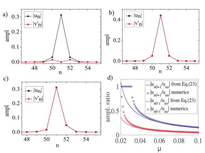
Figure 3: Numerical examples of fundamental nonlinear localized modes in the semi-infinite gap above the linear spectrum when $\Gamma=0.01$, $\sigma=0.005$, and $\mu=0.1$: spin-up mode (34) (a); spin-mixed mode (62) when $\mathfrak{a}=-0.5$ and $\theta=0$ (b); and spin-mixed mode (62) when $\mathfrak{a}=0$ and $\theta=\pi/2$ (c). Amplitude ratios between central and two neighboring sites obtained from numerics and Eq. (62) with $\theta=\pi/2$ for the continuation of the solution in (c) towards smaller $\mu$ are shown in (d).

Numerically calculated examples for the spin-up and spin-mixed modes are illustrated in Fig. 3. Note from (62) that, for the spin-mixed mode with $\theta=\pi/2$, $|u_{n_{0}+1}|^{2}+|v_{n_{0}+1}^{\prime}|^{2}\neq|u_{n_{0}-1}|^{2}+|v_{n_{0}-1}^{\prime}|^{2}$, i.e., the reflection symmetry around the central site gets broken on the opposite sublattice (upper or lower part of the chain) if there is a nontrivial phase-shift between the spin-up and spin-down components at the central site. As $|\Gamma\sigma|/\mu^{2}$ increases the spatial asymmetry increases (Fig. 3 (d)), until the solution typically bifurcates with an inter-site centered (two-site) mode with equal amplitudes at sites $n_{0}$ and $n_{0}+1$ before reaching the upper band edge at $\mu=2\Gamma$.

III.2 Fundamental gap modes from the flat-band limit

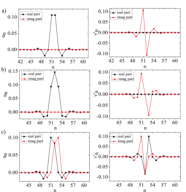
Figure 4: Numerical examples of $u_{n}$ and $v^{,}_{n}$ components of fundamental (type I) (a), type II (b) and type III (c) gap modes found in the mini-gap opened by the spin-orbit coupling when $\Gamma=0.01$, $\sigma=0.007$, $\mathfrak{a}=0.5$, and $\mu=0$.

Since the gap in the linear spectrum opened by the spin-orbit coupling at $k=\pm\pi/2$ appears only when $\Gamma$ and $\sigma$ are both nonzero, the standard anticontinuous limit $\Gamma=\sigma=0$ is not suitable for constructing nonlinear localized modes with frequency inside this gap (“discrete gap solitons”). Instead, we may use the flat-band limit $|\Gamma|=|\sigma|\neq 0$, where the exact nonlinear compacton modes (19)-(20) can be used as “building blocks” for the continuation procedure. Analogously to above, we may then calculate gap solitons perturbatively in the small parameter $|\Gamma|-|\sigma|$. To be specific, we assume $\mathfrak{a}>-1$, $\Gamma\geq\sigma>0$, and consider the continuation of a single two-site compacton from the lower flat band $\mu=-2\Gamma$ into the gap. From the limiting solution (19) with the upper sign, we then obtain the lowest-order corrections to six central sites (amplitudes at other sites are of higher order) as:

$$\left(\begin{array}[]{c}u_{n_{0}}\\ v_{n_{0}}^{\prime}\end{array}\right)\approx\sqrt{\frac{\mu+2\Gamma}{1+\mathfrak{a}}}\left(1-\frac{\Gamma-\sigma}{5\Gamma-\sigma+2\mu}\right)e^{-i\mu t}\left(\begin{array}[]{c}1\\ {i}\end{array}\right);\left(\begin{array}[]{c}u_{n_{0}+1}\\ v_{n_{0}+1}^{\prime}\end{array}\right)\approx\sqrt{\frac{\mu+2\Gamma}{1+\mathfrak{a}}}\left(1-\frac{\Gamma-\sigma}{5\Gamma-\sigma+2\mu}\right)e^{-i\mu t}\left(\begin{array}[]{c}1\\ {-i}\end{array}\right);$$ (72)

$$\left(\begin{array}[]{c}u_{n_{0}-1}\\ v_{n_{0}-1}^{\prime}\end{array}\right)\approx\sqrt{\frac{\mu+2\Gamma}{1+\mathfrak{a}}}\frac{\mu(\Gamma-\sigma)}{(\Gamma+\sigma)^{2}-\mu^{2}}e^{-i\mu t}\left(\begin{array}[]{c}1\\ {-i}\end{array}\right);\left(\begin{array}[]{c}u_{n_{0}+2}\\ v_{n_{0}+2}^{\prime}\end{array}\right)\approx\sqrt{\frac{\mu+2\Gamma}{1+\mathfrak{a}}}\frac{\mu(\Gamma-\sigma)}{(\Gamma+\sigma)^{2}-\mu^{2}}e^{-i\mu t}\left(\begin{array}[]{c}1\\ {i}\end{array}\right);$$ (81)

$$\left(\begin{array}[]{c}u_{n_{0}-2}\\ v_{n_{0}-2}^{\prime}\end{array}\right)\approx-\sqrt{\frac{\mu+2\Gamma}{1+\mathfrak{a}}}\frac{\Gamma^{2}-\sigma^{2}}{(\Gamma+\sigma)^{2}-\mu^{2}}e^{-i\mu t}\left(\begin{array}[]{c}1\\ {i}\end{array}\right)\left(\begin{array}[]{c}u_{n_{0}+3}\\ v_{n_{0}+3}^{\prime}\end{array}\right)\approx-\sqrt{\frac{\mu+2\Gamma}{1+\mathfrak{a}}}\frac{\Gamma^{2}-\sigma^{2}}{(\Gamma+\sigma)^{2}-\mu^{2}}e^{-i\mu t}\left(\begin{array}[]{c}1\\ {-i}\end{array}\right).$$ (90)

This family of fundamental gap modes (called type I gap modes) can be continued throughout the gap, with a numerical example illustrated in Fig. 4 (a). Profiles of another two types of gap modes numerically found to exist as nonlinear continuation of fundamental compactons, are depicted in Fig. 4 (b,c). Family of gap modes of type II (Fig. 4 (b)) originates from compact solution which is superposition of two neighboring overlapping in-phase compactons. On the other hand, type III gap modes evolve in the presence of nonlinearity from superposition of two neighboring overlapping compactons with a $\pi/2$ phase difference (Fig. 4 (c)).

IV Linear stability of nonlinear localized modes

Linear stability of the above modes can be checked from the standard eigenvalue problem. If we denote the amplitudes of the exact stationary modes of (17) as $\{u_{n}^{(0)},v_{n}^{\prime(0)}\}$, we may express the perturbed modes as $u_{n}=\left[u_{n}^{(0)}+(c_{n}e^{-i\lambda t}+d_{n}^{*}e^{i\lambda^{*}t})\right]e^{-i\mu t}$, $v_{n}^{\prime}=\left[v_{n}^{\prime(0)}+(f_{n}e^{-i\lambda t}+g_{n}^{*}e^{i\lambda^{*}t})\right]e^{-i\mu t}$. Inserting into (17) and linearizing, we obtain the following linear system of equations for the perturbation amplitudes $\{c_{n},d_{n},f_{n},g_{n}\}$:

$$\left(-\mu+2|u_{n}^{(0)}|^{2}+\mathfrak{a}|v_{n}^{\prime(0)}|^{2}\right)c_{n}+u_{n}^{(0)2}d_{n}+\mathfrak{a}u_{n}^{(0)}v_{n}^{\prime(0)*}f_{n}+\mathfrak{a}u_{n}^{(0)}v_{n}^{\prime(0)}g_{n}-\Gamma(c_{n+1}+c_{n-1})-i\sigma(f_{n+1}-f_{n-1})=\lambda c_{n}$$

$$\left(\mu-2|u_{n}^{(0)}|^{2}-\mathfrak{a}|v_{n}^{\prime(0)}|^{2}\right)d_{n}-u_{n}^{(0)*2}c_{n}-\mathfrak{a}u_{n}^{(0)*}v_{n}^{\prime(0)*}f_{n}-\mathfrak{a}u_{n}^{(0)*}v_{n}^{\prime(0)}g_{n}+\Gamma(d_{n+1}+d_{n-1})-i\sigma(g_{n+1}-g_{n-1})=\lambda d_{n}$$

$$\left(-\mu+2|v_{n}^{\prime(0)}|^{2}+\mathfrak{a}|u_{n}^{(0)}|^{2}\right)f_{n}+v_{n}^{\prime(0)2}g_{n}+\mathfrak{a}u_{n}^{(0)*}v_{n}^{\prime(0)}c_{n}+\mathfrak{a}u_{n}^{(0)}v_{n}^{\prime(0)}d_{n}+\Gamma(f_{n+1}+f_{n-1})-i\sigma(c_{n+1}-c_{n-1})=\lambda f_{n}$$

$$\left(\mu-2|v_{n}^{\prime(0)}|^{2}-\mathfrak{a}|u_{n}^{(0)}|^{2}\right)g_{n}-v_{n}^{\prime(0)*2}f_{n}-\mathfrak{a}u_{n}^{(0)*}v_{n}^{\prime(0)*}c_{n}-\mathfrak{a}u_{n}^{(0)}v_{n}^{\prime(0)*}d_{n}-\Gamma(g_{n+1}+g_{n-1})-i\sigma(d_{n+1}-d_{n-1})=\lambda g_{n}.$$

(91)

Linear stability is then equivalent to (91) having no complex eigenvalues. We may easily solve it for the uncoupled modes. Due to the overall gauge invariance of (17) ($u_{n}\rightarrow e^{i\phi}u_{n},v_{n}^{\prime}\rightarrow e^{i\phi}v_{n}^{\prime}$), there are always two eigenvalues at $\lambda=0$. For the spin-polarized modes, the remaining two eigenvalues are at $\lambda=\pm(1-\mathfrak{a})\mu$, while for the spin-mixed mode there is a fourfold degeneracy at $\lambda=0$. The latter is explained by the arbitrary phase difference $\theta$ between the $u$ and $v$ components for this mode.

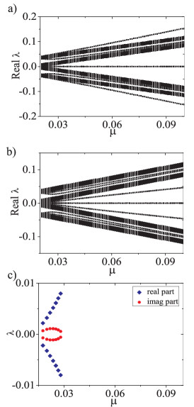
Figure 5: Stability eigenvalues for the continuation of fundamental spin-up states (34) when $\Gamma=0.01$, $\sigma=0.005$, and $\mathfrak{a}=-0.5$ (a), $\mathfrak{a}=0.5$ (b), and $\mathfrak{a}=1.5$ (c), respectively. For $\mathfrak{a}\leq 1$ the imaginary parts of eigenvalues are zero to numerical accuracy. Only the unstable eigenvalues are shown for $\mathfrak{a}=1.5$.

To see whether linear stability of the fundamental modes survives switching on the couplings $\Gamma,\sigma$, we first note that the linear spectrum of (91) corresponding to sites with $u_{n}^{(0)}\equiv v_{n}^{\prime(0)}\equiv 0$ has four branches, at $\lambda\in\pm[\mu-2\Gamma,\mu-2\sigma]$ and $\lambda\in\pm[\mu+2\sigma,\mu+2\Gamma]$. Thus, unless $\mathfrak{a}=0,1,\,\text{or}\,2$, we see immediately that the fundamental spin-polarized modes must remain linearly stable at least for small couplings. The general stability properties for larger $\Gamma$ and/or $\sigma$ will be discussed below for the different fundamental modes separately.

IV.1 Spin-polarized modes above the spectrum

Typical results from numerical diagonalization of (91) for the family of fundamental spin-polarized modes above the spectrum are shown in Fig. 5. As is seen, these modes are linearly stable in their full regime of existence when $\mathfrak{a}<1$. The magnitude of the frequency of the internal eigenmode arising from local oscillations at the central site lies above the linear spectrum when $\mathfrak{a}<0$ (Fig. 5 (a)) and below the linear spectrum when $0<\mathfrak{a}<1$ (Fig. 5 (b)). In both cases, it smoothly joins the band edge as $\mu\rightarrow 2\Gamma$ (linear limit), without causing any resonances. On the other hand, for $\mathfrak{a}>1$, the Krein signature of this eigenmode will change, as a consequence of the spin-polarized mode now having a lower energy than a spin-mixed mode, and thus it is no longer an energy maximizer for the system. This results in small regimes of weak oscillatory instabilities when the internal mode collides with the linear spectrum for frequencies close to the band edge, as shown in Fig. 5 (c).

IV.2 Spin-mixed modes above or below the spectrum

For the fundamental spin-mixed modes continued from (62), the four-fold degeneracy of zero eigenvalues resulting from the relative phase $\theta$ is generally broken for non-zero coupling as only modes with integer $2\theta/\pi$ can be continued, and moreover the structures of modes with $\theta=0$ and $\theta=\pi/2$ become non-equivalent. We discuss here first the case $\theta=0$, and show in Fig. 6 typical results from numerical diagonalization for different values of $\mathfrak{a}$.

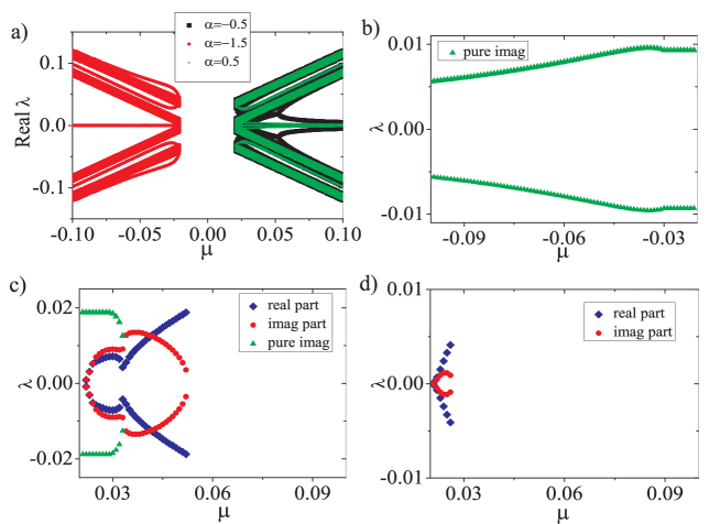
Figure 6: Stability eigenvalues for the continuation of fundamental spin-mixed states (62) with $\theta=0$ when $\Gamma=0.01$ and $\sigma=0.005$. (a) Real parts of eigenvalues when $\mathfrak{a}=-1.5$ (red (middle gray) circles), $\mathfrak{a}=-0.5$ (black squares), and $\mathfrak{a}=0.5$ (green (light gray) triangles), respectively. Unstable eigenvalues when $\mathfrak{a}=-1.5$ (b), $\mathfrak{a}=-0.5$ (c), and $\mathfrak{a}=0.5$ (d), respectively. Here, purely imaginary eigenvalues are represented by green (light gray) triangles, and complex eigenvalues are represented by blue (dark gray) squares and red (middle gray) circles for their real and imaginary parts, respectively.

First, for $\mathfrak{a}<-1$, as remarked above the spin-mixed modes lie below the linear spectrum ($\mu<-2\Gamma$), and the pair of eigenvalues originating from $\lambda=0$ in the anticontinuous limit ($\mu\rightarrow-\infty$) generally goes out along the imaginary axis (Fig. 6 (b)), where it remains. Thus, spin-mixed modes with $\theta=0$ and $\mathfrak{a}<-1$ are generically unstable. On the other hand, when $\mathfrak{a}>-1$ the spin-mixed modes lie above the linear spectrum ($\mu>2\Gamma$), and for $-1<\mathfrak{a}<1$ this eigenvalue pair goes out along the real axis (Fig. 6 (a)). Thus, these modes remain linearly stable for sufficiently large $\mu$ (or, equivalently, weak coupling), but become unstable through oscillatory instabilities (complex eigenvalues, see Figs. 6 (c,d)) as they approach the linear band edge with widening tails, causing resonances between the local oscillation mode at the central site and modes arising from oscillations at small-amplitude sites.

An example of the dynamics that may result from the oscillatory instabilities of the spin-mixed modes in this regime is shown in Fig. 7.

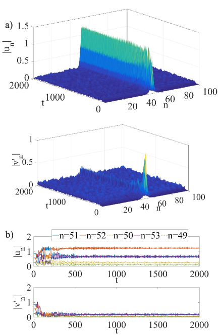
Figure 7: Direct numerical simulation of a slightly randomly perturbed spin-mixed mode with $\theta=0$ and $\mu=2.5$, when $\Gamma=1$, $\sigma=0.5$, and $\mathfrak{a}=0.5$. Evolution of $u_{n}$ and ${v^{,}_{n}}$ components (a) and dynamics of corresponding components given specifically for the five central sites (b).

Note that, after the initial oscillatory dynamics, the solution settles down at the stable fundamental spin-up mode (in this particular case the mode center is also shifted one site to the right).

As illustrated in Figs. 6 (c,d), the stability regime increases for $\mathfrak{a}$ increasing towards 1, and exactly at $\mathfrak{a}=1$ the spin-mixed states are always stable. However, for $\mathfrak{a}>1$ the eigenvalue pair originating from zero again goes out along the imaginary axis (not shown in Fig. 6) as for $\mathfrak{a}<-1$, and thus spin-mixed modes with $\theta=0$ are generally unstable also for $\mathfrak{a}>1$. In fact, this latter instability can be considered as a stability exchange with the $\theta=\pi/2$ spin-mixed mode, which, as illustrated in Fig. 8, is generally unstable with purely imaginary eigenvalues for $\mathfrak{a}<1$ (Figs. 8(a,b)) but stable for $\mathfrak{a}>1$ (Fig. 8(c)).

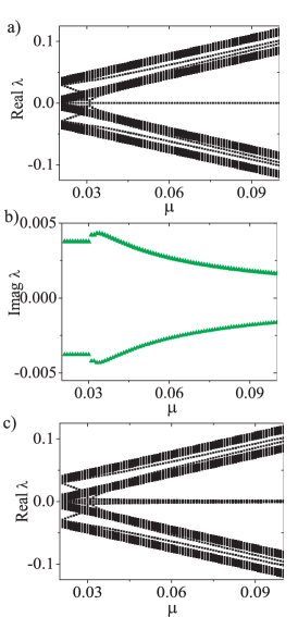
Figure 8: Stability eigenvalues for the continuation of fundamental spin-mixed states (62) with $\theta=\pi/2$ when $\Gamma=0.01$ and $\sigma=0.005$. Real (a) (Imaginary (b)) parts of eigenvalues when $\mathfrak{a}=0.5$. Eigenvalues when $\mathfrak{a}=1.5$ (c) (imaginary parts are zero to numerical accuracy).

IV.3 Compact modes in the flat-band limit

In the flat-band limit, we may obtain exact analytical expressions for the stability eigenvalues of the single two-site compacton modes. We focus as above on the specific case with $\Gamma=\sigma>0$ and $\mathfrak{a}>-1$, when the nonlinear compacton originating from $\mu=-2\Gamma$ (Eq. (19) with upper sign) enters the mini-gap for increasing $\mu$. For all zero-amplitude sites, the eigenvalues are just those corresponding to the flat-band linear spectrum, $\lambda=\pm\mu\pm 2\Gamma$. For the compacton sites, four eigenvalues correspond to local oscillations obtained by eliminating the surrounding lattice: $\lambda=0$ (doubly degenerate as always) and $\lambda=\pm 2\sqrt{2\Gamma(\mu+4\Gamma)}$. Since the eigenvalues of these internal modes are always real for $\Gamma>0$ and they do not couple to the rest of the lattice, they do not generate any instability. The remaining eigenvalues describe the modes coupling the perturbed compacton to the surrounding lattice, and are obtained from the subspace with $c_{n_{0}}=if_{n_{0}},d_{n_{0}}=-ig_{n_{0}},c_{n_{0}+1}=-if_{n_{0}+1},d_{n_{0}+1}=ig_{n_{0}+1}$. The rather cumbersome result can be expressed as:

$$\lambda^{2}=\frac{\mu^{2}}{2}+2\mu\Gamma\frac{1-\mathfrak{a}}{1+\mathfrak{a}}+2\Gamma^{2}\left(1+\frac{4}{1+\mathfrak{a}}\right)$$

$$\pm\left\{\frac{\mu^{4}}{4}-\frac{2\Gamma\mu^{3}(1-\mathfrak{a})}{1+\mathfrak{a}}+2\Gamma^{2}\mu^{2}\left[1+4\frac{(1-\mathfrak{a})^{2}-2}{(1+\mathfrak{a})^{2}}+\frac{4\mathfrak{a}}{1+\mathfrak{a}}\right]+\frac{8\Gamma^{3}\mu}{1+\mathfrak{a}}\left(1-\mathfrak{a}-\frac{8\mathfrak{a}}{1+\mathfrak{a}}\right)+4\Gamma^{4}\left[\left(1+\frac{4}{1+\mathfrak{a}}\right)^{2}-4\right]\right\}^{1/2}.$$ (92)

Oscillatory instabilities are generated if the expression inside the square-root in (92) becomes negative. Since obtaining explicit general expressions for instability intervals in $\mu$ would require solving a nontrivial fourth-order equation, we show in Fig. 9 numerical results for the specific parameter values $\mathfrak{a}=\pm 0.5$ and $1.5$.

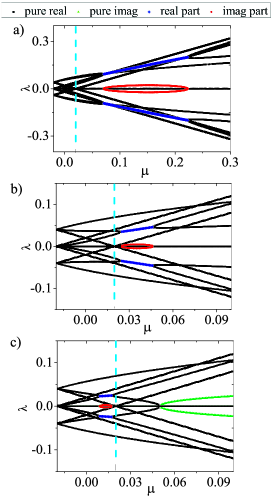
Figure 9: Stability eigenvalues for the compacton (19) with upper sign when $\Gamma=\sigma=0.01$, and $\mathfrak{a}=-0.5$ (a), $\mathfrak{a}=0.5$ (b), and $\mathfrak{a}=1.5$ (c), respectively. Purely real eigenvalues are represented in black, while green (light gray) colored symbols stand for purely imaginary ones. Complex eigenvalues are represented in blue (dark gray) and red (middle gray) for their real and imaginary parts, respectively. The blue dashed vertical line represents the upper gap edge.

As can be seen, the compacton remains stable throughout the mini-gap as long as $\mathfrak{a}\leq 1$ but develops an interval of oscillatory instability in the semi-infinite gap above the spectrum. The instability interval vanishes exactly at $\mathfrak{a}=1$, but then moves into the upper part of the mini-gap for $\mathfrak{a}>1$. Purely imaginary eigenvalues, resulting from the terms outside the square-root in (92) becoming negative, also appear in the semi-infinite gap for $\mathfrak{a}>1$.

IV.4 Gap modes in the mini-gap

For the fundamental (type I) gap mode continued from the single two-site compacton (90) (assuming again $\mathfrak{a}>-1$ and $\Gamma>\sigma>0$), we illustrate in Fig. 10(a) typical results for the numerical stability analysis.

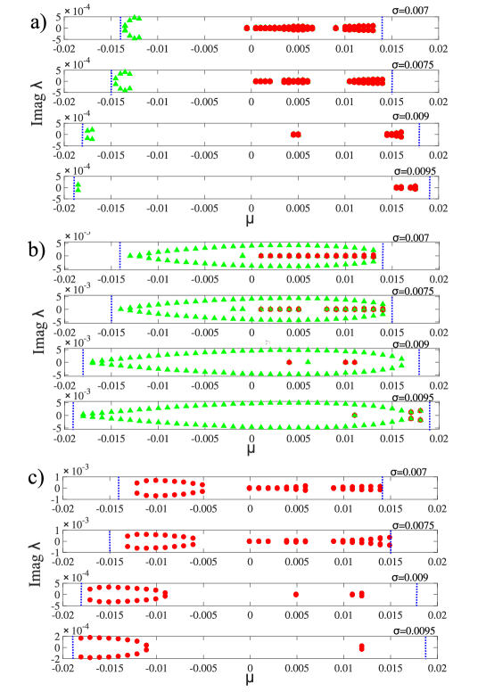
Figure 10: Imaginary parts of stability eigenvalues for the continuation of: fundamental (I type) (a), type II (b) and type III (c) gap mode inside the mini-gap, when $\Gamma=0.01$ and $\mathfrak{a}=0.5$. Pure imaginary eigenvalues are depicted with green (light gray) triangles, while red (dark gray) circles correspond to imaginary parts of complex eigenvalues. When $\sigma=0.01$, the eigenvalues for fundamental gap mode are those of the compacton illustrated in Fig. 9(b). From bottom to top, $\sigma$ is decreased to 0.007. Blue vertical dotted lines represent the locations of the lower and upper gap edges. Profiles of the corresponding solutions at $\sigma=0.007$ in the mid-gap ($\mu=0$) are depicted in Fig. 4.

As can be seen, as $\sigma$ decreases from the compacton limit $\sigma=\Gamma$, weak instabilities start to develop mainly close to the two gap edges. A further decrease in $\sigma$ yields instabilites in most of the upper half of the gap, while the mode remains stable in large parts of the lower half. Comparison with the stability eigenvalues for the exact compacton (Fig. 9(b)) shows that the instabilities in the upper part of the gap result from resonances between modes corresponding to compacton internal modes (92) and the continuous linear spectrum modes, which get coupled as the tail of the solution gets more extended. (These are seen in Fig. 9(b) as eigenvalue collisions at $\mu\approx 0.005$ and $\mu\approx 0.015$, but do not generate any instability in this figure since the corresponding eigenmodes are uncoupled in the exact compacton limit. However, they generate oscillatory instabilities when the exact compacton condition is not fulfilled, as seen in Fig. 10(a).) On the other hand, the instabilities appearing close to the lower gap edge, where the shape of the gap mode is far from compacton-like and closer to a continuum gap soliton (see Fig. 11 (a)) arise from purely imaginary eigenvalues. Direct numerical simulations of the dynamics in this regime (Fig. 11 (b)) shows that the main outcome of these instabilities is a spatial separation of the spin-up and spin-down components.

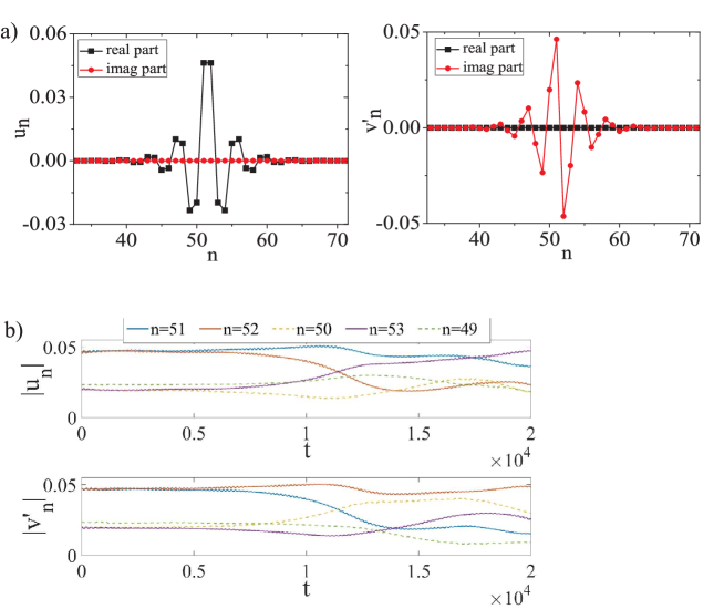
Figure 11: Profile of an unstable fundamental gap mode with $\Gamma=0.01,\mathfrak{a}=0.5,\sigma=0.007,\mu=-0.0125$ (a). Direct simulation of the dynamics when this mode is slightly perturbed; only five central sites are shown (b). Note the tendency for the spin-up and spin-down components to localize mainly on odd and even sites, respectively, after $t\sim 10^{4}$.

As for the type II gap modes that arise in the mini-gap from the superposition of two in-phase neighboring single compactons in the presence of nonlinearity, we obtained pure imaginary eigenvalues in the whole mini-gap, even for the case when value of $\sigma$ slightly differs from $\Gamma$ (see Fig. 10 (b)). Here, with further decrease of $\sigma$, eigenvalues related to oscillatory instabilities start to occur but only in the upper half of the mini-gap.

On the other hand, instability eigenvalue spectra for type III gap solutions contain only imaginary parts of complex eigenvalues (see Fig. 10 (c)). These instabilities are always present in the lower half of the mini-gap and expand to the upper part as we move further from the compacton limit.

V Conclusions

We derived the relevant tight-binding model for a zigzag-shaped chain of spin-orbit coupled exciton-polariton condensates, focusing on the case with basis functions of zero angular momentum and chain angles $\pm\pi/4$. The simultaneous presence of spin-orbit coupling and nontrivial geometry opens up a gap in the linear dispersion relation, even in absence of external magnetic fields. At particular parameter values, where the strength of the dispersive and spin-orbit nearest-neighbor couplings are equal, the linear dispersion vanishes, leading to two flat bands with associated compact modes localized at two neigboring sites.

We analyzed, numerically and analytically, the existence and stability properties of nonlinear localized modes, as well in the semi-infinite gaps as in the mini-gap of the linear spectrum. The stability of fundamental single-peaked modes in the semi-infinite gaps was found to depend critically on the parameter $\mathfrak{a}$ describing the relative strength of the nonlinear interaction between polaritons of opposite and identical spin (the latter assumed to be always repulsive). Generally, a spin-mixed mode with phase difference $\pi/2$ between spin-up and spin-down components is favoured when $\mathfrak{a}>1$ (cross-interactions repulsive and stronger than self-interactions), while a spin-polarized mode is favoured for $\mathfrak{a}<1$, which is the typical case in most physical setups. However, significant regimes of linear stability were found also for spin-mixed modes with zero phase difference between components when $|\mathfrak{a}|<1$, and for spin-polarized modes when $\mathfrak{a}>1$.

For parameter values yielding a flat linear band, nonlinear compactons appear in continuation of the linear compact modes, in the mini-gap as well as in the semi-infinite gaps. The linear stability eigenvalues for a single two-site compacton were obtained analytically, and shown to result in purely stable compactons inside the mini-gap when $\mathfrak{a}<1$, while regimes of instability were identified in the semi-infinite gaps, and when $\mathfrak{a}>1$ also inside the mini-gap. Continuing compact two-site modes away from the exact flat-band limit yields the exponentially localized fundamental nonlinear gap modes inside the mini-gap. Several new regimes of instability develop, but the fundamental gap modes typically remain stable in large parts of the lower half of the gap when $\mathfrak{a}<1$. We also found numerically nonlinear continuations of superpositions of two overlapping neighboring compactons (i.e., localized on three sites) with phase difference zero or $\pi/2$, where the latter also were found to exhibit significant regimes of linear stability in the mini-gap.

The model studied here may have an experimental implementation with exciton-polaritons in microcavities. Recently, microcavities have been actively investigated as quantum simulators of condensed matter systems. Polaritons have been proposed to simulate XY Hamiltonian Berloff-2017 , topological insulators Nalitov-Z ; Klembt18 , various types of lattices Nalitov-graphene ; Gulevich-kagome ; Klembt17 ; Lieb-2018 among other interesting proposals Sala-PRX-2015 many of which were realized experimentally. In fact, the quasi one-dimensional zigzag chain considered here may be a more practical system to study the effects of interactions in presence of spin-orbit coupling as compared to the full two-dimensional systems mentioned above. A possible realization of the studied system could be using microcavity pillars or tunable open-access microcavities Duff-APL-2014 . In the latter ones, large values of TE-TM splitting can be achieved exceeding that of monolithic cavities by a factor of three Dufferwiel15 . Apart from directly controlling the strength of TE-TM splitting by changing parameters of the experimental system such as the offset of the frequency from the center of the stop band of the distributed Bragg reflector Panzarini-PRB-1999 , one more possibility to control parameters of the system is provided by using the excited states of the zigzag nodes such as spin vortices which were shown to influence the sign of the coupling strength between the sites in a polaritonic lattice DY-graphene . To what extent it is also possible to realize the exact tight-binding flat-band condition derived here, i.e., to tune experimental parameter values so that the nearest-neighbor spin-orbit coupling coefficient $\sigma$ becomes equal to the standard dispersive nearest-neighbor overlap integral $\Gamma$ while hoppings beyond nearest neighbors remain negligible, is to the best of our knowledge an open question.

Finally, we note also the recent realizations of zigzag chains with large tunability for atomic Bose-Einstein condensates An18 , opening up the possibility for studying related phenomena involving spin-orbit coupling in a different context. Having in mind experimental progress on coherent transfer of atomic Bose-Einstein condensates into the flat bands originating from different optical lattice configurations (e.g., Taie ; Kang ), as well as in engineering spin-orbit coupling within ultracold atomic systems Lin ; Zhai , experimental realization of phenomena analogous to those described in the present work should be expected to be within reach. Very recently, a theoretical proposal for observing flat bands and compact modes for spin-orbit coupled atomic Bose-Einstein condensates in one-dimensional shaking optical lattices also appeared, where an exact tuning of the spin-orbit term could be achieved by an additional time-periodic modulation of the Zeeman field AS18 .

- (1) A.V. Kavokin, J.J. Baumberg, G. Malpuech, and F.P. Laussy, ”Microcavities” (Oxford, 2017).
- (2) M. Sich, D.V. Skryabin, D.N. Krizhanovskii, ”Soliton physics with semiconductor exciton-polaritons in confined systems,” Comptes Rendus Physique 17, 908-919 (2016).
- (3) C. Schneider, K. Winkler, M.D. Fraser, M. Kamp, Y. Yamamoto, E.A. Ostrovskaya, and S. Höfling, ”Exciton-polariton trapping and potential landscape engineering,” Rep. Prog. Phys. 80, 016503 (2017).
- (4) T. Ozawa et al., ”Topological Photonics”, https://arxiv.org/abs/1802.04173.
- (5) Y.V. Kartashov, and D.V. Skryabin, ”Bistable topological insulator with exciton-polaritons,” Phys. Rev. Lett. 119, 253904 (2017).
- (6) D.D. Solnyshkov, A.V. Navitov and G. Malpuech, Phys. Rev. Lett. 116, 046402 (2016).
- (7) H. Flayac, I.A. Shelykh, D.D. Solnyshkov, and G. Malpuech, Phys. Rev. B 81, 045318 (2010).
- (8) M. Sich, F. Fras, J.K. Chana, M.S. Skolnick, D.N. Krizhanovskii, A.V. Gorbach, R. Hartley, D.V. Skryabin, S.S. Gavrilov, E.A. Cerda-Méndez, K. Biermann, R. Hey, and P.V. Santos, Phys. Rev. Lett. 112, 046403 (2014).
- (9) M. Vladimirova, S. Cronenberger, D. Scalbert, K.V. Kavokin, A. Miard, A. Lemaître, J. Bloch, D. Solnyshkov, G. Malpuech, and A.V. Kavokin, Phys. Rev. B 82, 075301 (2010).
- (10) S. Dufferwiel et al., Phys. Rev. Lett. 115, 246401 (2015).
- (11) T. Zhang and G.-B. Jo, Scientific Reports 5, 16044 (2015).
- (12) A. Gagge, Cold p-band atoms in the zig-zag optical lattice: implementing a quantum simulator of next-nearest neighbor spin chains, M.Sc. Thesis, Stockholm University, 2016; http://www.fysik.su.se/jolarson/teaching/axel.pdf
- (13) M. Salerno and F.Kh. Abdullaev, Phys. Lett. A 379, 2252 (2015).
- (14) H. Sakaguchi and B.A. Malomed, Phys. Rev. E 90, 062922 (2014).
- (15) P.P. Beličev, G. Gligorić, J. Petrovic, A. Maluckov, Lj. Hadžievski, and B.A. Malomed, J. Phys. B: At. Mol. Opt. Phys. 48, 065301 (2015).
- (16) G. Gligorić, A. Maluckov, Lj. Hadžievski, S. Flach, and B.A. Malomed, Phys. Rev. B 94, 144302 (2016).
- (17) O. Derzhko, J. Richter, and M. Maksymenko Int. J. Mod. Phys. B 29, 1530007 (2015).
- (18) D. Leykam, A. Andreanov, and S. Flach, Adv. Phys.: X 3, 1473052 (2018).
- (19) D. Leykam, S. Flach, APL Photonics 3, 070901 (2018)
- (20) X. Li, E. Zhao, and W.V. Liu, Nat. Commun. 4:1523 (2013).
- (21) W. Maimaiti, A. Andreanov, H.C. Park, O. Gendelman, and S. Flach, Phys. Rev. B 95, 115135 (2017).
- (22) M. Johansson, U. Naether and R.A. Vicencio, Phys. Rev. E 92, 032912 (2015).
- (23) C. Danieli, A. Maluckov, and S. Flach, Low Temperature Physics/Fizika Nizkikh Temperatur 44, 865 (2018).
- (24) S. Darmanyan, A. Kobyakov, E. Schmidt, and F. Lederer, Phys. Rev. E 57, 3520 (1998).
- (25) N.G. Berloff, M. Silva, K. Kalinin, A. Askitopoulos, J.D. Töpfer, P. Cilibrizzi, W. Langbein, and P.G. Lagoudakis, Nat. Mater. 16, 1120 (2017).
- (26) A.V. Nalitov, D.D. Solnyshkov, and G. Malpuech, Phys. Rev. Lett. 114, 116401 (2015).
- (27) S. Klembt et al., Nature 562, 552 (2018).
- (28) A.V. Nalitov, G. Malpuech, H. Terças, and D.D. Solnyshkov, Phys. Rev. Lett. 114, 026803 (2015).
- (29) D.R. Gulevich, D. Yudin, I.V. Iorsh, and I.A. Shelykh, Phys. Rev. B 94, 115437 (2016).
- (30) S. Klembt et al., Appl. Phys. Lett. 111, 231102 (2017).
- (31) C.E. Whittaker et al., Phys. Rev. Lett. 120, 097401 (2018).
- (32) V.G. Sala, D.D. Solnyshkov, I. Carusotto, T. Jacqmin, A. Lemaître, H. Terças, A. Nalitov, M. Abbarchi, E. Galopin, I. Sagnes, J. Bloch, G. Malpuech, and A. Amo, Phys. Rev. X 5, 011034 (2015).
- (33) S. Dufferwiel et al., Appl. Phys. Lett. 104, 192107 (2014).
- (34) G. Panzarini et al., Phys. Rev. B 59, 5082 (1999).
- (35) D.R. Gulevich and D. Yudin, Phys. Rev. B 96, 115433 (2017).
- (36) F.A. An, E.J. Meier, and B. Gadway, Phys. Rev. X 8, 031045 (2018).
- (37) S. Taie, H. Ozawa, T. Ichinose, T. Nishio, S. Nakajima, and Y. Takahashi, Sci. Adv. 1, e1500854 (2015).
- (38) J.H. Kang, J.H. Han, and Y. Shin, arXiv:1807.01444 (2018).
- (39) Y.-J. Lin, K. Jiménez-García, and I.B. Spielman, Nature 471, 83 (2011).
- (40) H. Zhai, Rep. Prog. Phys. 78, 026001 (2015).
- (41) F. Kh. Abdullaev and M. Salerno, Phys. Rev. A 98, 053606 (2018).