Decay of semiclassical massless Dirac fermions from integrable and chaotic cavities

Abstract

Conventional microlasing of electromagnetic waves requires (1) a high $Q$ cavity and (2) a mechanism for directional emission. Previous theoretical and experimental work demonstrated that the two requirements can be met with deformed dielectric cavities that generate chaotic ray dynamics. Is it possible for a massless Dirac spinor wave in graphene or its photonic counterpart to exhibit a similar behavior? Intuitively, because of the absence of backscattering of associated massless spin-1/2 particles and Klein tunneling, confining the wave in a cavity for a long time seems not feasible. Deforming the cavity to generate classical chaos would make confinement even more difficult. Investigating the decay of a spin-1/2 wave from a scalar potential barrier defined cavity characterized by an effective refractive index $n$ that depends on the applied potential and the particle energy, we uncover the striking existence of an interval of the refractive index in which the average lifetime of the massless spin-1/2 wave in the cavity can be as high as that of the electromagnetic wave, for both integrable and chaotic cavities. We also find scaling laws for the ratio between the mean escape time associated with electromagnetic waves and that with massless spin-1/2 particles versus the index outside of this interval. The scaling laws hold regardless of the nature of the classical dynamics. All the results are verified numerically. The findings provide insights into the emergent field of Dirac electron optics and have potential applications in developing unconventional electronics using 2D Dirac materials.

I Introduction

Recent years have witnessed vast development of 2D Dirac materials such as graphene Novoselov et al. (2004, 2005); Neto et al. (2009), silicene and germanene Wehling et al. (2014); Wang et al. (2015). In these solid state materials, the energy-momentum relation (dispersion relation) of low-energy excitations is typically that of a relativistic quantum particle governed by the Dirac equation. For a massless spin-1/2 Dirac particle, the dispersion relation is linear which, for the positive energy band, is exactly that of a photon. It is natural to exploit principles in optics to articulate strategies to control Dirac electron flows. In this regard, various optically analogous phenomena such as Fabry-Pérot resonances Shytov et al. (2008); Rickhaus et al. (2013), Talbot effect Walls and Hadad (2016), and waveguide Williams et al. (2011); Rickhaus et al. (2015a) in ballistic graphene and similar Dirac materials have been demonstrated. Due to the negative energy band that has no counterpart for photons, the nontrivial $\pi$ Berry phase associated with conical band degeneracy and uniquely relativistic quantum behaviors such as Klein tunneling Klein (1929); Strange (1998); Katsnelson et al. (2006) can arise, leading to unusual physics such as the absence of backscattering Ando et al. (1998); Novikov (2007), high carrier mobility Geim and Novoselov (2007), and electrically controllable negative refractive index Cheianov et al. (2007). As a result, Dirac particles in ballistic graphene or other electronic honeycomb lattice crystals can exhibit a number of unconventional, optical-like behaviors such as negative Goos-Hänchen effect Beenakker et al. (2009), chirality-assisted electronic cloaking Gu et al. (2011), gate controlled caustics Cserti et al. (2007), electron Mie scattering Heinisch et al. (2013); Caridad et al. (2016); Gutiérrez et al. (2016); Lee et al. (2016a), and whispering gallery modes Wu and Fogler (2014); Zhao et al. (2015); Jiang et al. (2017); Ghahari et al. (2017). Optical-like devices for Dirac particles have also been realized, such as Klein-tunneling beam splitters and collimators Rickhaus et al. (2015b); Liu et al. (2017); Barnard et al. (2017) as well as microscopes Bãggild et al. (2017). In addition, the emergent internal degrees of freedom, i.e., sublattice and valley pseudospins as well as the electron spin, provide new possibilities for optics based electronic devices such as valley resolved waveguides Wu et al. (2011), beam splitters Settnes et al. (2016), electronic birefringent superlenses Asmar and Ulloa (2013), and spin (current) lenses Moghaddam and Zareyan (2010); Zhang et al. (2017). Quite recently, a Dirac quantum chimera state has been uncovered based on the electronic analog of the chiroptical effect Xu et al. (2018). Dirac electron optics Cserti et al. (2007); Cheianov et al. (2007); Du et al. (2008); Shytov et al. (2008); Beenakker et al. (2009); Moghaddam and Zareyan (2010); Gu et al. (2011); Williams et al. (2011); Rickhaus et al. (2013); Liao et al. (2013); Heinisch et al. (2013); Asmar and Ulloa (2013); Wu and Fogler (2014); Zhao et al. (2015); Rickhaus et al. (2015a); Lee et al. (2015); Rickhaus et al. (2015b); Walls and Hadad (2016); Caridad et al. (2016); Gutiérrez et al. (2016); Lee et al. (2016a); Chen et al. (2016); Settnes et al. (2016); Liu et al. (2017); Barnard et al. (2017); Jiang et al. (2017); Ghahari et al. (2017); Zhang et al. (2017); Bãggild et al. (2017); Xu et al. (2018) have thus become an active field of research.

While optical principles have been exploited in electronics, conventional optics and photonics have also greatly benefited from the development of Dirac electronics. For example, the photonic counterparts of Dirac materials such as graphene, topological insulators and Dirac Semimetals have been extensively studied, where light is structured in specific ways to mimic the Dirac particles through the rendering of photonic Dirac cone band structures. This has led to novel ways to control light with striking phenomena such as pseudospin-based vortex generation Song et al. (2015) and robust light transport Lu et al. (2014). Quite recently, inspired by the emergent topological properties uncovered in gapped Dirac electronic systems Haldane (1988), researchers have made breakthroughs in topological insulator lasers implemented by topological photonic cavities Bandres et al. (2018); Harari et al. (2018).

Uncovering, understanding, and exploiting the fundamental dynamics of Dirac particles are thus relevant to both Dirac electronics and photonics. In this paper, we investigate the trapping of massless Dirac particles in a scalar potential confinement and the escape from it to address the following question: is it possible for spin-1/2 Dirac spinor waves in graphene or photonic graphene systems to exhibit properties similar to those of photons in a microlasing cavity? To gain insights, we recall the conventional microlasing systems of electromagnetic waves in a dielectric cavity Nöckel et al. (1994); Mekis et al. (1995); Nöckel et al. (1996); Nöckel and Stone (1997), where the geometric shape of the cavity plays an important role in the wave decay. The dielectric constant of the cavity is higher than that of the surroundings, so total internal reflections are responsible for optical ray trapping. For a circular domain, the classical ray dynamics are integrable, leading to permanent ray trapping and in principle, to an infinite $Q$ value. However, in microlasing applications, emission of light is necessary, and one thus wishes to generate two seemingly contradictory behaviors at the same time: high $Q$ and good emission directionality. It was theoretically proposed Nöckel et al. (1994); Mekis et al. (1995); Nöckel et al. (1996); Nöckel and Stone (1997) and experimentally realized Gmachl et al. (1998) that classical chaos can be exploited to realize both behaviors at the same time, leading to high-$Q$ and highly efficient microcavity lasing. In nonlinear dynamics, the cavity problem is closely related to transient chaos Liu and Lai (2002); Lai and Tél (2011) and leaking Altmann et al. (2013), with the underlying physics being non-Hermitian Cao and Wiersig (2015). The main advantage that classical chaos can bring about is that, with simple deformation of the domain boundary, the phase space is “mixed” with coexistence of Kolmogorov-Arnold-Moser (KAM) tori and chaotic regions, leading to algebraic decay of light rays. The “long-tail” nature of the decay gives rise to a high $Q$ value, while the eventual escape from the chaotic component generates highly directional emission. In nonlinear dynamics, the exact form of the particle decay law depends on the relative “portion” of the phase space regions whose dynamics are quasiperiodic (KAM tori) or chaotic. While a mixed phase space gives rise to algebraic decay with the exponent depending on the amount of domain deformation, a fully chaotic phase space leads to exponential decay of light rays. Semiclassically, the cavity problem can be treated by using plane waves following Fresnel’s law, leading to the development of periodic theory of diffraction Vattay et al. (1994), understanding of emission properties in wave chaotic resonant cavities Narimanov et al. (1999); Altmann (2009), uncovering of wave scars Rex et al. (2002); Lee et al. (2002, 2004), analyses of the survival probability Ryu et al. (2006), directional emission Nöckel et al. (1996); Nöckel and Stone (1997); Wiersig and Hentschel (2008), and Goos-Hänchen effect Schomerus and Hentschel (2006). For conventional optics in microlasing cavities, a general principle is then that the nature of classical dynamics plays an important role in the decay law.

In order to realize microlasing like behavior, two requirements must be met: high $Q$ or long lifetime of the wave in the cavity and deformed geometry to ensure directional emission through classical chaos. Trapping of massless fermions has recently been experimentally realized in a graphene confinement Zhao et al. (2015); Gutiérrez et al. (2016); Lee et al. (2016b); Ghahari et al. (2017). The geometric shape of the confinement can be chosen to yield classically integrable, mixed, or chaotic dynamics. We note that, the system is essentially open with relativistic tunneling defined escape dynamics and thus generally support trapping modes with a finite lifetime Hewageegana and Apalkov (2008); Bardarson et al. (2009); Titov et al. (2010); Yang et al. (2011); Schneider and Brouwer (2011); Heinl et al. (2013); Schneider and Brouwer (2014). The problem is also different from that of scattering of Dirac particles from a potential barrier Wu and Fogler (2014); Xu and Lai (2016). We focus on the semiclassical regime in which the plane wave approximation is valid and Fresnel’s law is applicable. Intuitively, due to the total absence of backscattering of massless spin-1/2 particles Ando et al. (1998); Novikov (2007) and the purely relativistic quantum phenomenon of Klein tunneling Klein (1929); Strange (1998); Katsnelson et al. (2006), the decay of the spinor wave would be enhanced when comparing with that of classical electromagnetic waves from the same cavity, so trapping of the former would seem impossible. Indeed, a detailed scaling analysis of the ratio of the mean escape time of an electromagnetic wave to that of a spin-1/2 wave reveals that, for both integrable and chaotic cavities, in the regime of large effective refractive index values ($n\gg 1$), the ratio is proportional to $n$ but in the regime of $n\ll 1$, the ratio is inversely proportional to $n$. This means that, in these two asymptotic regimes, the averaging lifetime of the spin-1/2 wave is indeed much smaller than that of the electromagnetic wave. The surprising phenomenon is that, in between the two asymptotic regimes, an interval in $n$ emerges, in which the ratio is about one, indicating that the spin-1/2 wave can live as long as the electromagnetic counterpart. This means that, high $Q$ can be achieved for spin-1/2 particles. Since the constant ratio also holds for classical chaotic cavities, nonisotropic coherent emission can be expected. The finding suggests strongly that the two microlasing conditions for photons can be fulfilled for spin-1/2 particles. Our analysis provides insights into Dirac electronics and photonics, and has potential applications in developing unconventional cavity laser designs based on Dirac photonic crystals, and optical-like electronics with 2D Dirac materials.

We remark that, for photonic graphene systems Zhang and Liu (2008); Zandbergen and de Dood (2010); Bittner et al. (2010), the concept of lasing can be defined since the underlying particles are actually photons. For Dirac fermions, an analog is atom laser Bloch et al. (1999), that emits a beam of atoms (not light). Rigorously, the concept of “lasing” does not hold for an atom laser. In fact, traditional atom lasers require Bose Einstein condensate (BEC), although there was an attempt to generate an atom laser without BEC Reinaudi et al. (2006). In this paper, the term “lasing” is loosely used for photonic graphene systems. For Dirac fermions, we use the term “coherent emission.”

II Ray dynamics for spin-1/2 fermion

We focus on the semiclassical regime where the wavelength of the particle is relatively small in comparison with the size of the system but is non-negligible. In the semiclassical regime, both quantum and classical behaviors are relevant, and it is the ideal regime to study the quantum manifestations of distinct types of classical dynamics including chaos. In fact, most previous work in the traditional field of (nonrelativistic) quantum chaos Stöckmann (1999); Haake (2010) emphasizes the importance of the semiclassical regime.

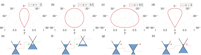
Figure 1: Approach of Dirac electron optics to solving the fermion decay problem: four distinct intervals of the effective refractive index in the domain of electrical potential confinement. (a-d) The transmission coefficient versus the incident angle in the polar representation for $n\in(-\infty,-1]$, $n\in[-1,0]$, $n\in[0,1]$, and $n\in[1,\infty)$, respectively. (e-h) The corresponding Dirac cone structures outside and inside of the confinement region. Note that, for (a,b) [or (e,f)], inside the potential region, the directions of the wavevector and the velocity are opposite to each other because of the negative refractive index in these two cases.

Trapping of a spin-1/2 fermion can be realized through a confinement (cavity) of electrical potential given by Gutiérrez et al. (2016)

$$V(\mathbf{r})=\begin{cases}0,&\mathbf{r}\in\mathcal{D},\\ V_{0},&\mathbf{r}\notin\mathcal{D},\\ \end{cases}$$ (1)

where $\mathcal{D}$ represents the geometrical domain of the cavity and $V_{0}$ is the uniform potential applied to the domain. Classically, the cavity is equivalent to a billiard, where the ray behavior is identical to that of a point particle bouncing back and forth in the billiard, with the difference that an optical ray is subject to reflection and refraction. The geometry shape of $\mathcal{D}$ can then be chosen to generate characteristically distinct types of classical dynamics: from integrable to fully chaotic. To be concrete, in this paper, we focus on two types of geometrical shapes for the cavity: a circle or a square that generates classically integrable dynamics and a stadium in which the classical dynamics are chaotic. Experimentally, for a 2D solid state material (e.g., graphene), the domain $\mathcal{D}$ can be realized through the technique of scanning tunneling microscope (STM) Zhao et al. (2015); Gutiérrez et al. (2016); Lee et al. (2016b); Ghahari et al. (2017).

The traditional theoretical approach consists of writing down the non-Hermitian Hamiltonian and solving the Dirac equation subject to proper boundary conditions Hewageegana and Apalkov (2008). If the domain shape is simple and highly symmetric, e.g., a circle, which yields classically integrable dynamics, then the solutions of the Dirac equation can be readily obtained. When the boundaries of the domain are deformed from the circular shape to generate chaotic dynamics, if the boundary conditions are of the infinite mass confinement type, numerical solutions of the Dirac equation can be obtained using the boundary integral method Berry and Mondragon (1987) or the standard finite element algorithm Ni et al. (2012). In our problem of particle trapping and decay, the boundary condition is not of the infinite mass confinement type. In this case, for a domain of an arbitrary shape, even numerical solutions of the Dirac equation are extremely difficult. Since our focus is on the semiclassical regime, we take advantage of the field of Dirac electron optics to solve the Dirac equation by using the approach of ray tracing associated with conventional wave optics.

When an electromagnetic wave encounters a boundary, reflection and refraction occur as governed by Fresnel’s law. In the underlying ray picture, there will be energy loss associated with each encounter with the domain boundary. For a spin-1/2 fermion, Klein tunneling must be taken into account to derive the corresponding Fresnel’s law. Depending on the particle energy $E$ relative to the potential height $V_{0}$, there are two distinct cases Allain and Fuchs (2011); Ozawa et al. (2017): (i) $0<E<V_{0}$ and (ii) $V_{0}<E$. In the first case ($0<E<V_{0}$), the transmission and reflection coefficients, $T$ and $R$, respectively, at each encounter with the boundary are given by Allain and Fuchs (2011); Ozawa et al. (2017)

$$T = -\frac{2\cos{\theta}\cos{\theta_{t}}}{1-\cos{(\theta+\theta_{t})}},$$ (2)

$$R = \frac{1+\cos{(\theta-\theta_{t})}}{1-\cos{(\theta+\theta_{t})}},$$

where $\theta$ is the incident angle with respect to the normal and the transmitted angle is given by

$$\theta_{t}=\sin^{-1}{\left(\frac{E}{E-V_{0}}\sin{\theta}\right)}+\pi=\sin^{-1}{(n\sin{\theta})}+\pi.$$ (3)

with the effective refractive index $n$ defined as $n\equiv E/(E-V_{0})$, which is negative in this case: $n\in(-\infty,0]$.

For the second case $V_{0}<E$, the transmission and reflection coefficients are given by

$$T = \frac{2\cos{\theta}\cos{\theta_{t}}}{1+\cos{(\theta+\theta_{t})}},$$ (4)

$$R = \frac{1-\cos{(\theta-\theta_{t})}}{1+\cos{(\theta+\theta_{t})}},$$

where the refracted angle is

$$\theta_{t}=\sin^{-1}{(n\sin{\theta})},$$ (5)

and the effective refractive index is positive: $n\in[0,\infty)$.

The energy band structure associated with a spin-1/2 fermion is that of a pair of Dirac cones. Depending on the relative positions of the Dirac cone structures outside and inside of the potential domain, there are four distinct intervals of the refractive index: $(-\infty,-1]$, $[-1,0]$, $[0,1]$ and $[1,\infty)$. Figures 1(a-d) show the transmission coefficient versus the incident angle in the polar representation for the four parameter intervals, respectively. The corresponding energy band structures are shown in Figs. 1(e-h), respectively.

The survival probability of a spin-1/2 fermion inside the potential region can be calculated using the formulas for the transmission and reflection coefficients. In general, the coefficients in the Klein tunneling regime depend on the incident energy $E$ and the potential height $V_{0}$ (which together define the effective refractive index $n$ Allain and Fuchs (2011)) as well as the angle of incidence $\theta$. There is a symmetry in the coefficients in that they do not depend on the sign of $n$, which can be seen by substituting the expression of $\theta_{t}$ into Eq. (2) or Eq. (4). It thus suffices to focus on the two distinct intervals of the values of the refractive index: $|n|<1$ and $|n|>1$. For $|n|>1$, total internal reflection can occur with the critical incident angle of $\theta_{c}$, where the transmission coefficient is zero for $\theta>\theta_{c}$.

III Results

Say we distribute an ensemble of rays of spin-1/2 waves with different initial conditions in the cavity. As a ray evolves following Fresnel’s law, its intensity will decrease due to refraction. Let $I_{0}$ be the initial intensity (or energy) of any ray in the ensemble. After $n$ encounters with the boundary, the intensity becomes

$$I_{n}=I_{0}\prod_{i}R_{i}=I_{0}\exp\left(\sum_{i}\ln R_{i}\right).$$ (6)

The survival probability $P(t)$ is the fraction of the remaining intensity at time $t$. Depending on the nature of the classical ray dynamics (integrable or chaotic) and on the value of the effective refractive index $n$, with time $P(t)$ decays either exponentially:

$$P(t)=\exp(-\gamma t),$$ (7)

where $\gamma$ is the exponential decay rate, or algebraically:

$$P(t)\sim t^{-z},$$ (8)

with $z$ being the algebraic decay exponent.

In numerical simulations, we initialize a large number of rays (between $10^{5}$ and $10^{7}$) randomly distributed on the boundary. For each ray, the initial angle $\theta_{0}$ is chosen according to $p=\sin{\theta_{0}}$, where $p$ is a uniform random variable in the unit interval and the velocity is chosen to be one. The final distribution of the rays is independent of the initial random conditions Lai and Tél (2011). In the following, we treat integrable and chaotic cavities separately.

III.1 Integrable cavity

We consider a circular cavity with integrable ray dynamics, in which the incident angle $\theta$ is constant and the time interval between two successive encounters with the boundary is $\Delta t=2\cos{(\theta)}$. For $|n|<1$, the ray intensity decays exponentially. As indicated in Fig. 1, the transmission coefficient $T$ takes on the minimum value at $\theta=\pi/2$. A ray with $\theta=\pi/2$ can thus survive in the cavity for a long time.

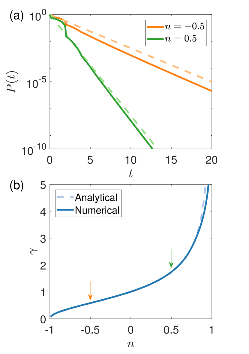
Figure 2: Exponential decay of the survival probability for the integrable (circular) cavity for $-1<n<1$. (a) Two examples of exponential decay of $P(t)$ ($n=-0.5$ and $n=0.5$). (b) The exponential decay exponent $\gamma$ versus $n$. Insofar as the value of $n$ is not close to one, the whispering gallery mode decays most slowly. For $n\rightarrow 1$, the cavity becomes transparent so $\gamma\rightarrow\infty$.

For $0<n<1$, the survival probability is given by

$$P(t)=\frac{\sum_{i}R_{i}^{t/\Delta t}}{N}=\lim_{\theta\rightarrow\pi/2}\left(\frac{1-\cos(\theta-\theta_{t})}{1+\cos(\theta+\theta_{t})}\right)^{t/(2\cos\theta)}.$$ (9)

Letting $x=\frac{\pi}{2}-\theta$, we expand $P(t)$ at $x=0$ to obtain

$$P(t)\approx\exp\left(-\frac{\sqrt{1-n^{2}}}{1-n}t\right).$$ (10)

The survival probability for $-1<n<0$ has the same exponential form but with different values of the decay exponent. Figure 2(a) shows the decay of the survival probability $P(t)$ with time for $n=-0.5$ and $n=0.5$ on a semi-logarithmic scale. Each set of data can be well fitted by a straight line, indicating that the decay is exponential. In both cases, the mode that survives the longest possible time in the cavity is the whispering gallery mode with $\theta\lesssim\pi/2$, and this holds insofar as the value of $n$ is not too close to one. Figure 2(b) shows, for $-1<n<1$, the exponential decay exponent $\gamma$ versus $n$. For $n\rightarrow 1$, the electrical potential vanishes, so the cavity becomes transparent, resulting in infinitely fast decay, i.e., $\gamma\rightarrow\infty$.

For $n>1$, total internal reflections occur for $\theta>\theta_{c}=\sin^{-1}{(1/n)}$. In this case, the modes that can survive for a long time are those with incident angle near $\theta_{c}$, and $P(t)$ is given by

$$P(t)=\frac{\int_{0}^{\theta_{c}}\cos{\theta}\exp{\left[-G(\theta)t\right]}d\theta}{\int_{0}^{1/n}dp},$$ (11)

where

$$G(\theta)=\frac{1}{2\cos{\theta}}\ln{\left(1+\frac{2\cos{\theta}\cos{\theta_{t}}}{1-\cos{(\theta-\theta_{t})}}\right)}.$$ (12)

Letting $x=\theta_{c}-\theta$, we have

$$G(\theta)\approx\alpha\sqrt{x}+O(x).$$ (13)

where

$$\alpha=\frac{n\sqrt{2\sqrt{n^{2}-1}}}{n-1}.$$ (14)

Substituting Eq. (13) into Eq. (11), we get

$$P(t) \approx \frac{2\sqrt{n^{2}-1}}{\alpha^{2}t^{2}}[1-(1+\alpha\sqrt{\theta_{c}}t)e^{-\alpha\sqrt{\theta_{c}}t}]$$ (15)

$$\approx \frac{2\sqrt{n^{2}-1}}{\alpha^{2}}t^{-2}.$$

We thus see that the decay of $P(t)$ for $n>1$ is algebraic. A similar analysis gives that Eq. (15) holds for the $n<-1$ region. Numerical validation of Eq. (15) is given in Fig. 3.

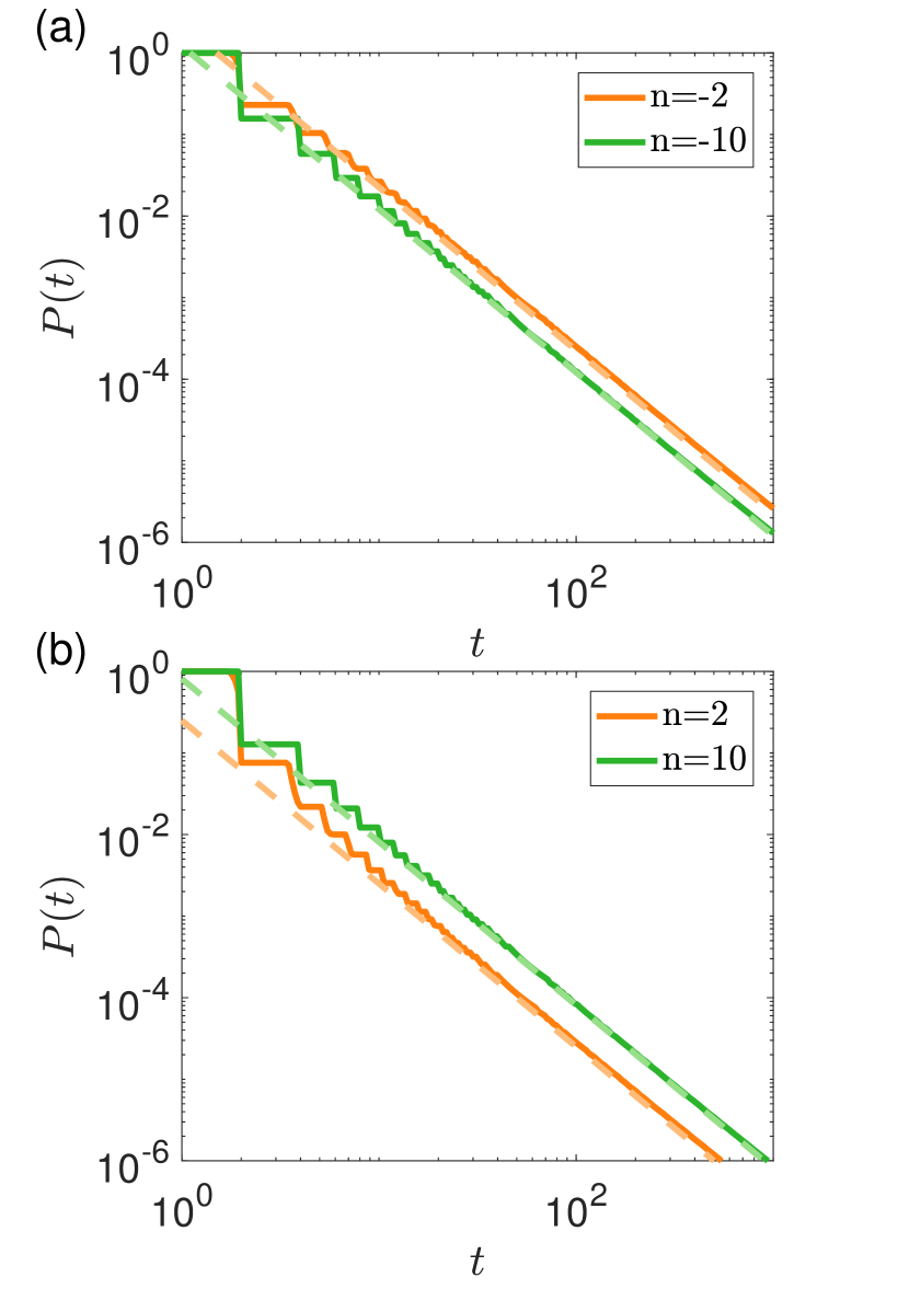
Figure 3: Algebraic decay of the survival probability for the integrable (circular) cavity for $|n|>1$. Shown are decay behaviors of $P(t)$ for (a) $n=-2$ and $n=-10$ and (b) $n=2$ and $n=10$. The solid and dashed lines represent numerical and theoretical results, respectively.

The special parameter point $n=1$ is one at which the decay law changes characteristically from being exponential to being algebraic. This is not surprising because of the emergence of total internal reflections for $n>1$. Another special parameter value is $n=-1$, which occurs when the particle energy is one half of the potential height: $E=V/2$. In this case, the transmission coefficient at a single encounter with the cavity boundary is $T=\cos^{2}{\theta}$, so the critical incident angle is $\theta_{c}=\pi/2$. Near $\theta_{c}$, the quantity $n\sin\theta_{c}$ can no longer be treated as a small number, so the expansion used in deriving Eq. (15) is not valid. However, we can rewrite $G(\theta)$ as

$$G(\theta)=-\frac{1}{2\cos\theta}\ln(1-\cos^{2}\theta).$$ (16)

For $\theta\rightarrow\pi/2$, we have $\cos{\theta}\sim x$ and obtain

$$P(t)\approx\int_{0}^{\pi/2}x\exp\left(-\frac{tx}{2}\right)d\theta=\frac{4}{t^{2}},$$ (17)

which is valid in the large $t$ regime.

III.2 Effect of Klein tunneling on decay of spin-1/2 wave

In terms of the cavity decay dynamics, what is the key difference between an electromagnetic wave and a Dirac spinor wave? For a Dirac particle, there is a fundamental phenomenon that has no counterpart for a photon: Klein tunneling Klein (1929); Strange (1998), a uniquely relativistic quantum phenomenon by which a particle of energy less than the height of a potential barrier can tunnel through it with absolute certainty. For a Dirac electron optical system, Klein tunneling occurs in the $|n|<1$ regime for $\theta=0$ because, from Eq. (2), we have $T(\theta=0)=1$. In this regime, the decay of both spin-1/2 and electromagnetic waves is exponential (see Table 1 below). However, the slowest decaying modes are quite different for the two types of waves. In particular, for the spin-1/2 wave they are the whispering gallery modes (corresponding to $\theta\approx\pi/2$) as it is difficult for the modes with $\theta\approx 0$ to stay in the cavity for a long time because of Klein tunneling. For the electromagnetic wave, the situation is nearly opposite: the longest survival modes are those with $\theta$ near zero, i.e., modes with propagation along the diameter of the cavity, as the transmission coefficients are minimum for them by Fresnel’s law.

To further appreciate the difference between the decay dynamics of spin-1/2 and electromagnetic waves, we study the ring cavity with a kind of a small “forbidden” region at the center of the circular cavity ($r<r_{1}<1$). The basic idea is that, the presence of the forbidden region should not have a significant impact on the decay of a spin-1/2 wave as the dominant surviving modes are of the whispering gallery type, which do not pass through the central region of the cavity. However, the forbidden region would affect the decay of the electromagnetic wave as the modes that shape the decay behavior are diametrical, which have a significant presence in the central region. The ring cavity is defined as

$$n(r)=\begin{cases}\infty,&r\leq r_{1},\\ (0,1),&r_{1}<r\leq 1,\\ 1,&r>1,\end{cases}$$ (18)

which is integrable. In terms of the ray dynamics, the central circular region blocks most orbits along the diameter. Figure 4(a) shows, for spin-1/2 wave and $n=0.9$, the exponential decay of the survival probability $P(t)$ for four different ring configurations (corresponding to different values of $r_{1}$) on a semi-logarithmic scale. The decay curves can be fitted approximately by lines with nearly identical slopes, indicating that introducing a central forbidden region has little effect on the decay. Figure 4(b) displays the curves of the exponential decay exponent $\gamma$ versus $n$ (for $0<n<1$) for the four different ring configurations, which are nearly identical. Figures 4(c) and 4(d) present the corresponding results for a TM electromagnetic wave (Appendix A), revealing a significant effect of the central forbidden region on the wave decay behavior. In particular, the decay rates for the three cases of $r_{1}\neq 0$ (orange, green and red curves) are greater than that of the circular cavity ($r_{1}=0$, the blue curve) because the central forbidden region blocks the slowest decaying modes so as to expedite the overall decay. The results for a TE electromagnetic wave are shown in Figs. 4(c) and 4(d), revealing an even more significant effect of the blockage of the central region on wave decay.

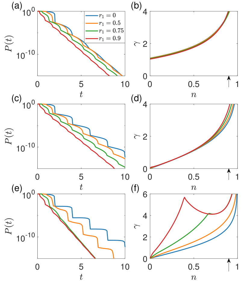
Figure 4: Decay of spin-1/2 and electromagnetic waves from a ring cavity. (a) For four different ring configurations ($r_{1}=0$ - the original circular cavity, $r_{1}=0.5$, 0.75, and 0.9), exponential decay behavior of the survival probability $P(t)$, and (b) the corresponding decay exponent $\gamma$ versus $n$ for $0<n<1$. As the long time decay behavior is dominated by the whispering gallery modes that concentrate on the larger circumstance, the central forbidden region has little effect on the overall exponential decaying behavior. (c,d) The corresponding results for a TM electromagnetic wave, where the decay rates for the three actual ring configurations are larger than that of the original circular cavity, due to the blockage of the slowest decaying modes along the diameter. (e,f) Results for a TE electromagnetic wave, where the inaccessibility of the central region has an even more significant impact on the decay.

Experimentally, for a spin 1/2 wave system, e.g., graphene, the central circular region can be created by applying an electrical potential corresponding exactly to the Fermi energy $E$. For the electromagnetic wave, the ring configuration can be realized by depositing metal in the central region of a circular dielectric cavity, which induces total internal reflections.

III.3 Chaotic cavity

To be concrete, we consider the chaotic stadium cavity characterized by parameters $r_{0}$ (the radius of each semicircle) and $L$ (the perimeter of the whole domain). It is useful to define Mortessagne et al. (1993) the “average path length” $\langle d\rangle=\pi A/L$, where $A$ is the area of the stadium. The survival probability is given by

$$P(t)=\prod_{i}R_{i}=\exp{\left[\frac{t}{\langle d\rangle}\sum_{i}\ln{R_{i}}\right]},$$ (19)

where $R_{i}$ is the reflection coefficient at each encounter with the boundary. The summation can be approximated by a double integral in both distance and angle. Due to chaos, the distance between two successive encounters with the boundary is roughly constant ($\langle d\rangle$), so the double integral can be reduced to a single integral with respect to the angle. The summation in Eq.(19) can then be evaluated as

$$\frac{\int_{0}^{\pi/2}\cos{\theta}\ln{R}d\theta}{\int_{0}^{\pi/2}\cos{\theta}d\theta}.$$ (20)

In general, the integral cannot be evaluated analytically. However, in the limiting cases ($|n|\rightarrow 0$ and $|n|\rightarrow\infty$), we can use Taylor expansion to evaluate the integral. The end result is an exponential decay of $P(t)$ (Appendix B) with explicit formulas for the decay exponent $\gamma$. In particular, for $n\rightarrow 0$, $\gamma$ is given by

$$\gamma=\frac{1}{\langle d\rangle}\left(\sum_{i=1}^{\infty}\frac{W_{2i+1}}{i}+\frac{\pi}{2}n\right),$$ (21)

where $W$ is the Walli’s integral (Appendix B). For $n\rightarrow\infty$, we have

$$\gamma=\frac{(8-2\pi)\pi r_{0}}{\langle d\rangle|n|L}.$$ (22)

Numerical verification is presented in Figs. 5. These results suggest that the decay of a spin-1/2 fermion from a chaotic cavity is generally exponential, implying the difficulty in confining the relativistic quantum particle.

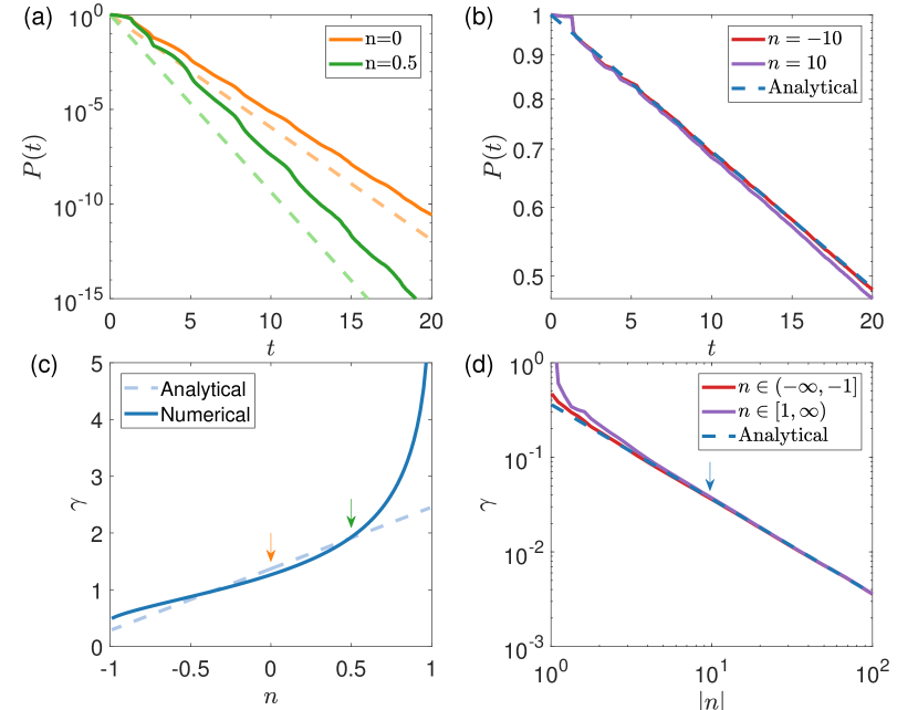
Figure 5: Exponential decay of a spin-1/2 fermion from a chaotic stadium cavity. (a) The survival probability $P(t)$ for $n=0$ and $n=0.5$ (on a semi-logarithmic scale), where the dashed lines are theoretical predictions. (b) Exponential decay of $P(t)$ for $n=-10$ and $n=10$. (c) The exponential decay exponent $\gamma$ versus $n$ for $-1<n<1$. (d) The exponent $\gamma$v versus $|n|$ for $1<|n|<100$. In (c) and (d), the dashed line is the analytic prediction. The parameters of the chaotic stadium are $A=\pi$, $r_{0}/l=1/2$, and $L=2\pi r_{0}+2l$, where $l$ is the length of the straight segment.

III.4 Are high $Q$ and nonisotropic coherent emission achievable for a spin-1/2 wave?

Two conditions must be met in order for a microcavity to generate effective lasing: (1) high $Q$ value, and (2) directional emission. Previous work on conventional electromagnetic microlasing Nöckel et al. (1994); Mekis et al. (1995); Nöckel et al. (1996); Nöckel and Stone (1997); Gmachl et al. (1998) established that deformed chaotic cavities are suited for microlasing applications. To realize microlasing of a spin-1/2 wave, it is necessary that (1) the (graphene) cavity has average lifetime comparable to that of the dielectric electromagnetic cavity, and (2) the lifetime can be maintained in a deformed chaotic cavity. In the following, we establish the existence of a range of the effective refractive index value for a spin-1/2 particle cavity in which the two requirements can be met.

To compare the decay of the spin-1/2 wave with that of the electromagnetic wave in the same cavity, it is necessary to have a complete picture of the decay of the electromagnetic wave from a cavity for comparison. Especially, for a spin-1/2 particles, in principle the relative refractive index $n$ can take on values ranging from $-\infty$ to $+\infty$. For electromagnetic waves, previous work Ryu et al. (2006) treated this problem but for the case where the absolute value $|n|$ of the relative refractive index of the dielectric cavity is greater than one, with the result that the decay law is algebraic (exponential) for integrable (chaotic) cavities. As a necessary step, we extend the result to the $|n|<1$ regime (Appendix A). Table 1 lists the formulas of $P(t)$ for both spin-1/2 and electromagnetic waves (TE and TM) for both integrable and chaotic cavities.

Table 1: Complete results of the survival probability for spin-1/2, TE and TM electromagnetic waves for integrable and chaotic cavities. For algebraic decay, the exact form of $P(t)$ is listed. For exponential decay, only the decay exponent $\gamma$ is given.

	Circular cavity		Stadium cavity
	$|n|<1$	$|n|>1$	$|n|<1$	$|n|>1$
Spin 1/2	$\gamma=\frac{\sqrt{1-n^{2}}}{1-n}$	$P(t)=\frac{(n-1)^{2}}{n^{2}}t^{-2}$	$\gamma=\sum_{i}\frac{W_{2i+1}}{\langle d\rangle i}+\frac{\pi n}{2\langle d\rangle}$	$\gamma=\frac{(8-2\pi)\pi r_{0}}{\langle d\rangle|n|L}$
TM	$\gamma=\ln\left(\frac{1+n}{1-n}\right)$	$P(t)=\frac{(n^{2}-1)^{2}}{4n^{2}}t^{-2}$	$\gamma=\frac{n\pi}{\langle d\rangle}$	$\gamma=\frac{2\pi^{2}r_{0}}{\langle d\rangle Ln^{2}}$
TE	$\gamma=\ln\left(\frac{1+n}{1-n}\right)$	$\gamma=\ln\left(\frac{n+1}{n-1}\right)$	$\gamma=\frac{2n\pi}{\langle d\rangle}$	$\gamma=\frac{4\pi^{2}r_{0}}{\langle d\rangle Ln^{2}}$

For the cavity decay problem, a basic characterizing quantity is the quality factor $Q$, which qualitatively measures the stability of the wave (temporarily) “trapped” in the cavity. To calculate the $Q$ value, we resort to the fact that, because the system is fundamentally open, the underlying Hamiltonian is non-Hermitian with complex eigenvalues, and $Q$ is nothing but the ratio between the real and imaginary parts of the complex eigen wave vector. Alternatively, $Q$ can be defined as $Q\equiv\omega_{n}\tau$, where $\omega$ is the frequency of the dominantly surviving mode, $\tau$ is the associated (finite) lifetime, and its inverse is the spectral width Cao and Wiersig (2015). In the ray picture, it is convenient to calculate the mean escape time (or lifetime) $T$, which is the time for $P(t)$ to reduce to the value of, e.g., $e^{-1}$.

Intuitively, because of Klein tunneling, it would be “easier” for a spin-1/2 wave to leak out of the cavity than an electromagnetic wave. Let $\tau_{\mbox{\tiny S}}$, $\tau_{\mbox{\tiny TE}}$, and $\tau_{\mbox{\tiny TM}}$ denote the mean escape time for spin-1/2, TE and TM electromagnetic waves, respectively. We analyze the ratios $\tau_{\mbox{\tiny TE}}/\tau_{\mbox{\tiny S}}$ and $\tau_{\mbox{\tiny TM}}/\tau_{\mbox{\tiny S}}$, which can be calculated based on the results in Table 1.

For the $|n|\ll 1$ regime, all three systems exhibit exponential decay, so we have $\tau=1/\gamma$. For electromagnetic waves, the average lifetime is proportional to $1/n$ but for the spin-1/2 system the time tends to a constant. We thus have

$$\tau_{\mbox{\tiny EM}}/\tau_{\mbox{\tiny S}}\sim\frac{1}{n}\gg 1\ \text{for}\ n\rightarrow 0,$$ (23)

for the integrable cavity, where $\tau_{\mbox{\tiny EM}}$ stands for either $\tau_{\mbox{\tiny TE}}$ or $\tau_{\mbox{\tiny TM}}$. The same result holds for the chaotic cavity. In this case, comparing with the electromagnetic wave, a spin-1/2 wave will leak out of the cavity more quickly, i.e., it is less “stable” when being compared with the electromagnetic wave.

In the $|n|\gg 1$ regime, for the integrable cavity, we have $P(t)\sim n^{2}t^{-2}$ for the TM electromagnetic wave, so the mean escape time $T_{\mbox{\tiny TM}}$ is proportional to $n$. For the TE wave, the decay is exponential with the exponent given by $\gamma=\ln{(n+1)/(n-1)}$. We thus have $\gamma\approx 2/n$ and, hence, $\tau_{\mbox{\tiny TE}}\sim n$, as for the TM wave. For the chaotic cavity, for both TM and TE waves, we have $\gamma\sim n^{-2}$, while $\gamma\sim n$ for spin-1/2 wave. We thus have $\tau_{\mbox{\tiny EM}}/\tau_{\mbox{\tiny S}}\sim n$, which means that, in the $|n|\gg 1$ regime, the $Q$ value of the electromagnetic cavity is also higher than that of the spin-1/2 Dirac cavity.

The analytic results can be summarized as

$$\begin{split}\tau_{\mbox{\tiny EM}}/\tau_{\mbox{\tiny S}}=\alpha_{1}n^{-1}\ \text{for}\ n\ll 1,\\ \tau_{\mbox{\tiny EM}}/\tau_{\mbox{\tiny S}}=\alpha_{2}n\ \text{for}\ n\gg 1,\end{split}$$ (24)

where $\alpha_{1}$ and $\alpha_{2}$ are constants that depend on the geometric shape of the cavity. We see that the integrable and chaotic cavities share the same scaling law of the lifetime ratios with the refractive index. Figures 6(a) and 6(b) show the numerically obtained ratios $\tau_{\mbox{\tiny TM}}/\tau_{\mbox{\tiny S}}$ and $\tau_{\mbox{\tiny TE}}/\tau_{\mbox{\tiny S}}$ versus $n$, respectively. There is a good agreement between the numerical results and those in Eq. (24). The remarkable result is that, while the decay of the spin-1/2 wave is significantly faster than that of the electromagnetic wave in both the $n\ll 1$ and $n\gg 1$ regimes, there exists a sizable interval about $n=1$ in which the decay rates of the two types of systems are comparable, as shown in Figs. 6(a,b). In this interval, high $Q$ values can be achieved for spin-1/2 particles. The striking phenomenon is that the ratios in this interval can be maintained at values close to one, regardless of the nature of the classical ray dynamics. That is, high $Q$ values can be achieved for spin-1/2 particles in a chaotic cavity to the same extent as for electromagnetic waves so as to ensure nonisotropic emission.

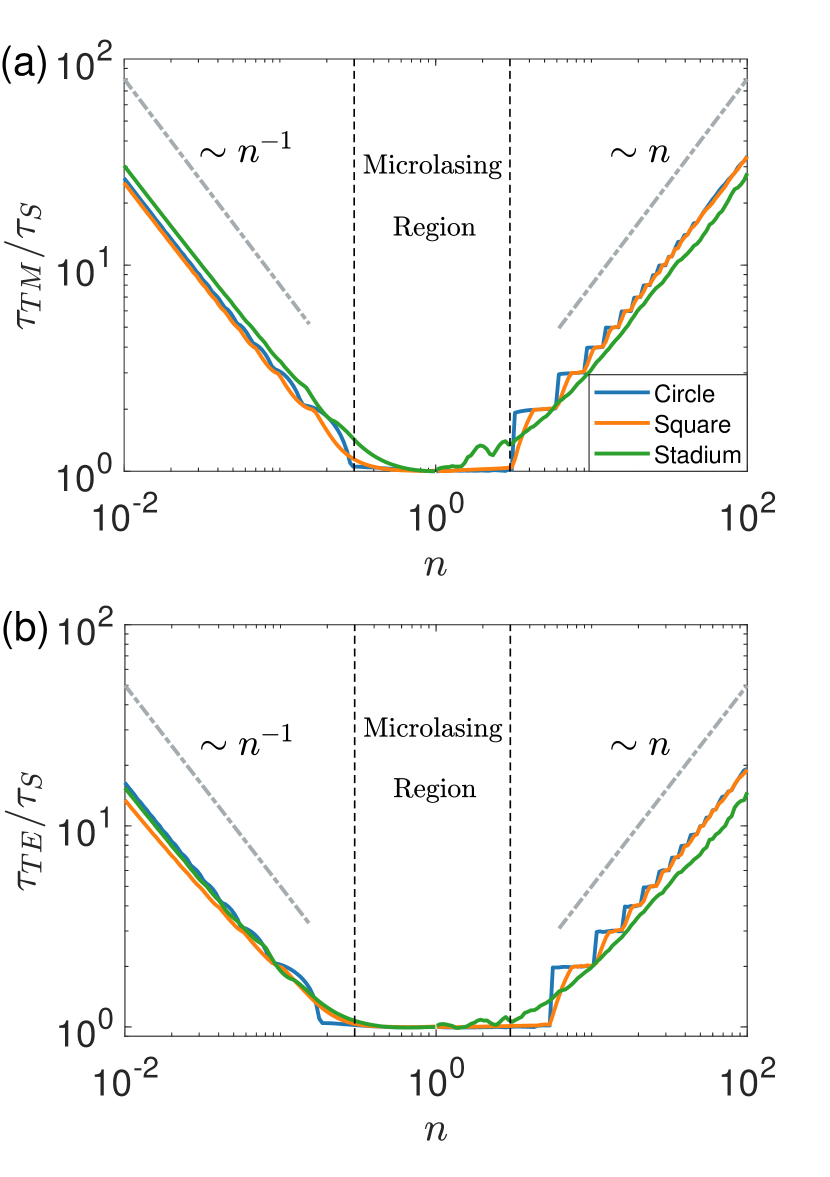
Figure 6: Scaling with the relative refractive index of the ratio between the mean escape time for an electromagnetic wave and that of a spin-1/2 wave: (a) the ratio $\tau_{\mbox{\tiny TM}}/\tau_{\mbox{\tiny S}}$ and (b) the ratio $\tau_{\mbox{\tiny TE}}/\tau_{\mbox{\tiny S}}$, for three different types of cavity shapes (two with integrable and one with chaotic ray dynamics). For $n\ll 1$, the ratio is proportional to $n^{-1}$ while it is proportional to $n$ for $n\gg 1$, regardless of whether the electromagnetic wave in comparison is TM or TE. The scaling laws hold regardless of whether the classical ray dynamics are integrable or chaotic. The surprising result is the existence of an interval in $n$ in which the spin-1/2 wave can have a high $Q$ value and chaos enabled directional emission as for the electromagnetic wave.

IV Discussion

To summarize, motivated by the question of whether high $Q$ and directional coherent emission are achievable for spin-1/2 particles, we investigated the cavity decay problem with classically distinct dynamics in the semiclassical regime. Previous work on microlasing of electromagnetic waves Nöckel et al. (1994); Mekis et al. (1995); Nöckel et al. (1996); Nöckel and Stone (1997); Gmachl et al. (1998) established that deformed chaotic cavities can meet the two key requirements for microlasing: high $Q$ value and effective directional emission. For spin-1/2 particles, confinement can be realized through an external electric field. Our analysis and numerical results indicate that, for a spin-1/2 wave cavity (e.g., made of graphene), there exists an experimentally reasonable range of the applied electric potential in which the two requirements can be met. For example, a chaotic graphene cavity can simultaneously have a high $Q$ value and good emission directionality.

More specifically, we have analyzed the survival probability in both integrable and chaotic cavities. For the integrable cavity, the decay is exponential in the $|n|<1$ regime. Significantly better confinement in the sense of algebraic decay of the survival probability can be achieved for the integrable cavity in the $|n|>1$ regime. For larger $n$ values (when the Fermi energy is close to the potential), confinement is more robust. This result is consistent with that obtained through wave scattering analysis Heinl et al. (2013) and also agrees with experimental measurement on circular potential confinement Zhao et al. (2015) where high quality confinement is achieved for high angular momentum modes. For the chaotic cavity, the survival probability decays exponentially with time for all possible $n$ values. We note, however, that the quantum regime in which the scattering theory is applicable is not the semiclassical regime treated in our work. In fact, in previous work on confinement of spin-1/2 fermions in graphene Katsnelson et al. (2006); Bardarson et al. (2009); Schneider and Brouwer (2011); Heinl et al. (2013); Schneider and Brouwer (2014), the relevant wave regime is not close to being semiclassical. To search for regimes where high $Q$ and nonisotropic coherent emission are possible for spin-1/2 particles, we obtain analytic formulas to compare the average lifetime with that of an electromagnetic wave in the same cavity. A striking result is that the behavior of the ratio of the average lifetimes of the two types of waves versus $|n|$ is independent of the nature of the underlying classical ray dynamics. For both $|n|\ll 1$ and $|n|\gg 1$ regimes, there are scaling laws governing the ratio, which indicates that the average trapping time of the electromagnetic wave is significantly longer than that of the spin-1/2 wave, in accordance with intuition. However, counter intuitively, there exists a regime of $|n|$ values centered about one in which the average lifetimes for the two types of waves are approximately the same, which is valid for both integrable and chaotic cavities, generating remarkable decaying behavior of a spin-1/2 wave in this regime.

We provide a brief discussion about the issue of directional emission. In optical microcavities, directional emission is typically shape dependent. For example, in Sec. VII of Ref. [Cao and Wiersig, 2015], a number of high-Q cavities were described, which are able to emit light in certain directions. For some specific cavity shape, it is possible to determine the probability of directional emission through ray tracing. For example, in Ref. [Wiersig and Hentschel, 2008], a heart shaped cavity was studied, where the emission direction depends on some long lasting orbits with initial incident angle $|\sin\theta|<1/n$. As ray trajectories associated with these orbits escape, radiation is generated but is concentrated in some special direction. In general, ray tracing is insufficient for determining if the underlying cavity can have directional emission. Instead, a wave approach based on scattering and solutions of the Dirac equation is necessary. Since a spin-1/2 system exhibits similar characteristics in the dependence of the transmission on the angle to those of light (e.g., the transmission reaches a maximum for $\theta=0$ and a minimum for $\theta=\theta_{c}$), it is possible for high-Q operation in spin-1/2 systems to possess directional emission.

We would also like to explain the difference between the results from a relevant recent work Xu et al. (2018) and those in the current work. Specifically, Ref. [Xu et al., 2018] treated a scattering problem in graphene systems, where the spin degeneracy of the electrons is lifted through an exchange field from induced ferromagnetism. The scattering region has a non-concentric type of ring geometry, where a different gate potential is applied to the inner circle and to the region outside the inner circle but within the outer circle, respectively. As a result, the scattering dynamics for spin-up and spin-down electrons are characteristically different, both classically and quantum mechanically. For example, for proper values of the gate potentials and eccentricity, the classical dynamics of spin-down electrons are completely integrable, while spin-up electrons exhibit fully developed chaotic scattering. Not only are the classical dynamics distinct, the corresponding quantum scattering also exhibits drastically different characteristics in terms of experimentally accessible quantities such as the cross sections, resonances, and the Wigner-Smith delay time. In Ref. [Xu et al., 2018], the simultaneous coexistence of two different types of scattering behaviors is coined by the term “relativistic quantum chimera.”

The focus of the current work is on optical like decay behaviors of Dirac fermions in the semiclassical regime in the absence of any induced ferromagnetism. There is then no splitting of the Dirac cone structure, i.e., the energy bands of spin-up and spin-down electrons are completely degenerate, ruling out the possibility of any relativistic quantum chimera state. The results reported here on the decay of semiclassical massless Dirac fermions from integrable or chaotic cavities thus do not depend on the electron spin. Also note that, in Ref. [Xu et al., 2018], while the classical dynamics were obtained using the same approach of Dirac electron optics as in the current work, the quantum scattering dynamics were calculated and analyzed based on solutions of the Dirac equation for two-component spinor waves.

Appendix A Survival probability of electromagnetic waves

For TM electromagnetic waves, the reflection coefficient is given by Jackson (1999)

$$R_{\mbox{\tiny TM}}(\theta)=\left(\frac{n\cos{\theta}-\cos{\theta_{t}}}{n\cos{\theta}+\cos{\theta_{t}}}\right)^{2},$$ (25)

where $\theta$ and $\theta_{t}$ are the incident and refractive angles, respectively, and $n$ is the relative refractive index. The formula for TE waves is

$$R_{\mbox{\tiny TE}}(\theta)=\left(\frac{\cos{\theta}-n\cos{\theta_{t}}}{\cos{\theta}+n\cos{\theta_{t}}}\right)^{2}.$$ (26)

The law of refraction is $\theta_{t}=\sin^{-1}{(n\sin{\theta})}$. For conventional dielectric materials, we have $n>0$.

Integrable cavity with $n<1$.

In contrast to spin-1/2 waves where whispering gallery modes survive in the cavity for the longest time [Eq. (9)], for TM and TE electromagnetic waves, such modes are along the diameter with $\theta=0$. Substituting $\theta=0$ into Eqs. (25) and (26), from Eq. (9), we obtain the orbit length as $2\cos{\theta}$ and the exponential decay exponent $\gamma$ as

$$\gamma_{\mbox{\tiny TM}}=\gamma_{\mbox{\tiny TE}}=\ln\left(\frac{1+n}{1-n}\right).$$ (27)

Integrable cavity with $n>1$.

We expand Eq. (13) near $\theta_{c}$ to obtain

$$G(\theta)\approx\alpha x^{1/2}+O(x).$$ (28)

where

$$\alpha_{\mbox{\tiny TM}}=\frac{2n\sqrt{2\sqrt{n^{2}-1}}}{n^{2}-1}.$$ (29)

The survival probability for a TM wave is

$$P(t)=\frac{2\sqrt{n^{2}-1}}{\alpha_{\mbox{\tiny TM}}^{2}}t^{-2}.$$ (30)

Similarly, we have, for a TE wave,

$$\alpha_{\mbox{\tiny TE}}=n^{2}\alpha_{\mbox{\tiny TM}}.$$ (31)

Chaotic stadium cavity with $n<1$.

Using $R(n=0)=1$ for all $\theta$, we expand $\ln{(1-T)}$ in the small $n$ regime to obtain

$$T=4n\cos\theta+O(n^{2}).$$ (32)

The integral in Eq. (20) can be evaluated as

$$-\int_{0}^{\pi/2}\ln{R\cos{\theta}}d\theta=\int_{0}^{\pi/2}4n\cos^{2}{\theta}d\theta=n\pi.$$ (33)

For a TE wave, the integral is

$$-\int_{0}^{\pi/2}\ln{R\cos{\theta}}d\theta=\int_{0}^{\pi/2}4nd\theta=2n\pi.$$ (34)

Chaotic stadium cavity with $n>1$.

The result can be found in Ref. [Ryu et al., 2006]. For a TM wave, the integral in Eq. (20) is

$$-\int_{0}^{\sin^{-1}{(1/n)}}\cos{\theta}\ln{(1-R)}\approx\pi n^{-2}.$$ (35)

For a TE wave, the integral is

$$-\int_{0}^{\sin^{-1}{(1/n)}}\cos{\theta}\ln{(1-R)}\approx 2\pi n^{-2}.$$ (36)

The exponential decay exponents $\gamma$ for the two cases are given by

$$\gamma_{\mbox{\tiny TM}} = \frac{2\pi^{2}r_{0}}{\langle d\rangle Ln^{2}},\ \mbox{and}$$ (37)

$$\gamma_{\mbox{\tiny TE}} = \frac{4\pi^{2}r_{0}}{\langle d\rangle Ln^{2}}.$$ (38)

Appendix B Survival probability of spin 1/2 waves in chaotic stadium cavity

The case of $|n|<1$.

For $n=0$, the reflection coefficient $R$ is

$$R=\frac{1-\cos{\theta}}{1+\cos{\theta}}.$$ (39)

We thus have

$$-\ln R=2\left(\frac{\cos^{2}{\theta}}{2}+\frac{\cos^{4}{\theta}}{4}+\cdots\right).$$ (40)

The ray density is given approximately by $\cos{\theta}$. Using Wallis’ integral Sebah and Gourdon (2002)

$$W_{n}=\int_{0}^{\pi/2}\cos^{n}{x}dx=\frac{\Gamma\left(\frac{n+1}{2}\right)\Gamma\left(\frac{1}{2}\right)}{2\Gamma\left(\frac{n}{2}+1\right)}.$$ (41)

we can evaluate the integral in Eq. (20) as

$$-\int\ln(R)\cos{\theta}d\theta=\sum_{n=1}^{\infty}\frac{W_{2n+1}}{n},$$ (42)

where $\lim_{n\rightarrow\infty}W_{n}=0$, so the series converges. For small $n$ values, we have

$$R\approx\frac{1-\cos{\theta}-n\sin^{2}{\theta}}{1+\cos{\theta}-n\sin^{2}{\theta}}.$$ (43)

Rewriting this as $R=R_{0}\left[1+nf(\theta)\right]$, we have the reflection coefficient for $n=0$ as

$$\ln{R}=\ln{R_{0}}+nf(\theta).$$ (44)

where

$$f(\theta)=\frac{n\sin^{2}{\theta}}{1+\cos{\theta}}-\frac{n\sin^{2}{\theta}}{1-\cos{\theta}}.$$ (45)

The decay exponent $\gamma$ can be determined through

$$-\int\cos\theta\ln R=\sum_{i=1}^{\infty}\frac{W_{2i+1}}{i}+\frac{\pi}{2}n.$$ (46)

The case of $|n|>1$.

For $|n|>1$, rays with incident angle near the critical value for total internal reflection dominate the long time behavior of the survival probability. Near the critical angle where $T$ is about zero, we can expand Eq. (20) as

$$-\int_{0}^{\pi/2}\cos{\theta}\ln(1-T)d\theta=\int_{0}^{\sin^{-1}{(1/n)}}T\cos{\theta}d\theta.$$ (47)

For $n\rightarrow\infty$, we let $p=n\sin\theta$ and expand the integrand in terms of $1/n$ to obtain

$$\frac{1}{n}\int_{0}^{1}\frac{2\sqrt{1-\frac{p^{2}}{n^{2}}}\sqrt{1-p^{2}}}{1+\sqrt{1-\frac{p^{2}}{n^{2}}}\sqrt{1-p^{2}}-\frac{p^{2}}{n}}dp\approx\frac{4-\pi}{n}.$$ (48)

The result at the $n\rightarrow-\infty$ limit is the same. We obtain

$$\gamma=\frac{(8-2\pi)\pi R}{\langle d\rangle|n|L}.$$ (49)

References

- Novoselov et al. (2004) K. S. Novoselov, A. K. Geim, S. V. Morozov, D. Jiang, Y. Zhang, S. V. Dubonos, I. V. Grigorieva, and A. A. Firsov, Science 306, 666 (2004).
- Novoselov et al. (2005) K. S. Novoselov, A. K. Geim, S. V. Morozov, D. Jiang, M. I. Katsnelson, I. V. Grigorieva, S. V. Dubonos, and A. A. Firsov, Nature 438, 197 (2005).
- Neto et al. (2009) A. H. C. Neto, F. Guinea, N. M. R. Peres, K. S. Novoselov, and A. K. Geim, Rev. Mod. Phys. 81, 109 (2009).
- Wehling et al. (2014) T. Wehling, A. Black-Schaffer, and A. Balatsky, Adv. Phys. 63, 1 (2014).
- Wang et al. (2015) J. Wang, S. Deng, Z. Liu, and Z. Liu, Nat. Sci. Rev. (2015), 10.1093/nsr/nwu080.
- Shytov et al. (2008) A. V. Shytov, M. S. Rudner, and L. S. Levitov, Phys. Rev. Lett. 101, 156804 (2008).
- Rickhaus et al. (2013) P. Rickhaus, R. Maurand, M.-H. Liu, M. Weiss, K. Richter, and C. Schönenberger, Nat. Commun. 4, 2342 (2013).
- Walls and Hadad (2016) J. D. Walls and D. Hadad, Sci. Rep. 6, 26698 (2016).
- Williams et al. (2011) J. R. Williams, T. Low, M. S. Lundstrom, and C. M. Marcus, Nat. Nanotech. 6, 222 (2011).
- Rickhaus et al. (2015a) P. Rickhaus, M.-H. Liu, P. Makk, R. Maurand, S. Hess, S. Zihlmann, M. Weiss, K. Richter, and C. Schonenberger, Nano Lett. 15, 5819 (2015a).
- Klein (1929) O. Klein, Zeitschrift für Physik 53, 157 (1929).
- Strange (1998) P. Strange, Relativistic Quantum Mechanics: with Applications in Condensed Matter and Atomic Physics (Cambridge University Press, Cambridge UK, 1998).
- Katsnelson et al. (2006) M. Katsnelson, K. Novoselov, and A. Geim, Nat. Phys. 2, 620 (2006).
- Ando et al. (1998) T. Ando, T. Nakanishi, and R. Saito, J. Phys. Soc. Jpn. 67, 2857 (1998).
- Novikov (2007) D. S. Novikov, Phys. Rev. B 76, 245435 (2007).
- Geim and Novoselov (2007) A. K. Geim and K. S. Novoselov, Nat. Mater. 6, 183 (2007).
- Cheianov et al. (2007) V. V. Cheianov, V. Fal’ko, and B. L. Altshuler, Science 315, 1252 (2007).
- Beenakker et al. (2009) C. W. J. Beenakker, R. A. Sepkhanov, A. R. Akhmerov, and J. Tworzydło, Phys. Rev. Lett. 102, 146804 (2009).
- Gu et al. (2011) N. Gu, M. Rudner, and L. Levitov, Phys. Rev. Lett. 107, 156603 (2011).
- Cserti et al. (2007) J. Cserti, A. Pályi, and C. Péterfalvi, Phys. Rev. Lett. 99, 246801 (2007).
- Heinisch et al. (2013) R. L. Heinisch, F. X. Bronold, and H. Fehske, Phys. Rev. B 87, 155409 (2013).
- Caridad et al. (2016) J. Caridad, S. Connaughton, C. Ott, H. B. Weber, and V. Krstic, Nat. Commun. 7, 12894 (2016).
- Gutiérrez et al. (2016) C. Gutiérrez, L. Brown, C.-J. Kim, J. Park, and A. N. Pasupathy, Nat. Phys. 12, 1069 (2016).
- Lee et al. (2016a) J. Lee, D. Wong, J. Velasco Jr, J. F. Rodriguez-Nieva, S. Kahn, H.-Z. Tsai, T. Taniguchi, K. Watanabe, A. Zettl, F. Wang, L. S. Levitov, and M. F. Crommie, Nat. Phys. 12, 1032 (2016a).
- Wu and Fogler (2014) J.-S. Wu and M. M. Fogler, Phys. Rev. B 90, 235402 (2014).
- Zhao et al. (2015) Y. Zhao, J. Wyrick, F. D. Natterer, J. F. Rodriguez-Nieva, C. Lewandowski, K. Watanabe, T. Taniguchi, L. S. Levitov, N. B. Zhitenev, and J. A. Stroscio, Science 348, 672 (2015).
- Jiang et al. (2017) Y. Jiang, J. Mao, D. Moldovan, M. R. Masir, G. Li, K. Watanabe, T. Taniguchi, F. M. Peeters, and E. Y. Andrei, Nat. Nanotech. 12, 1045 (2017).
- Ghahari et al. (2017) F. Ghahari, D. Walkup, C. Gutiérrez, J. F. Rodriguez-Nieva, Y. Zhao, J. Wyrick, F. D. Natterer, W. G. Cullen, K. Watanabe, T. Taniguchi, L. S. Levitov, N. B. Zhitenev, and J. A. Stroscio, Science 356, 845 (2017).
- Rickhaus et al. (2015b) P. Rickhaus, P. Makk, K. Richter, and C. Schonenberger, Appl. Phys. Lett. 107, 251901 (2015b).
- Liu et al. (2017) M.-H. Liu, C. Gorini, and K. Richter, Phys. Rev. Lett. 118, 066801 (2017).
- Barnard et al. (2017) A. W. Barnard, A. Hughes, A. L. Sharpe, K. Watanabe, T. Taniguchi, and D. Goldhaber-Gordon, Nat. Commun. 8, 15418 (2017).
- Bãggild et al. (2017) P. Bãggild, J. M. Caridad, C. Stampfer, G. Calogero, N. R. Papior, and M. Brandbyge, Nat. Commun. 8, 15783 (2017).
- Wu et al. (2011) Z. Wu, F. Zhai, F. M. Peeters, H. Q. Xu, and K. Chang, Phys. Rev. Lett. 106, 176802 (2011).
- Settnes et al. (2016) M. Settnes, S. R. Power, M. Brandbyge, and A.-P. Jauho, Phys. Rev. Lett. 117, 276801 (2016).
- Asmar and Ulloa (2013) M. M. Asmar and S. E. Ulloa, Phys. Rev. B 87, 075420 (2013).
- Moghaddam and Zareyan (2010) A. G. Moghaddam and M. Zareyan, Phys. Rev. Lett. 105, 146803 (2010).
- Zhang et al. (2017) S.-H. Zhang, J.-J. Zhu, W. Yang, and K. Chang, 2D Mater. 4, 035005 (2017).
- Xu et al. (2018) H.-Y. Xu, G.-L. Wang, L. Huang, and Y.-C. Lai, Phys. Rev. Lett. 120, 124101 (2018).
- Du et al. (2008) X. Du, I. Skachko, A. Barker, and E. Y. Andrei, Nat. Nanotech. 3, 491 (2008).
- Liao et al. (2013) B. Liao, M. Zebarjadi, K. Esfarjani, and G. Chen, Phys. Rev. B 88, 155432 (2013).
- Lee et al. (2015) G.-H. Lee, G.-H. Park, and H.-J. Lee, Nat. Phys. 11, 925 (2015), letter.
- Chen et al. (2016) S. Chen, Z. Han, M. M. Elahi, K. M. M. Habib, L. Wang, B. Wen, Y. Gao, T. Taniguchi, K. Watanabe, J. Hone, A. W. Ghosh, and C. R. Dean, Science 353, 1522 (2016).
- Song et al. (2015) D. Song, V. Paltoglou, S. Liu, Y. Zhu, D. Gallardo, L. Tang, J. Xu, M. Ablowitz, N. K. Efremidis, and Z. Chen, Nat. Commun. 6, 6272 (2015).
- Lu et al. (2014) L. Lu, J. D. Joannopoulos, and M. Soljaää, Nat. Photon. 8, 821 (2014).
- Haldane (1988) F. D. M. Haldane, Phys. Rev. Lett. 61, 2015 (1988).
- Bandres et al. (2018) M. A. Bandres, S. Wittek, G. Harari, M. Parto, J. Ren, M. Segev, D. N. Christodoulides, and M. Khajavikhan, Science 359 (2018), 10.1126/science.aar4005.
- Harari et al. (2018) G. Harari, M. A. Bandres, Y. Lumer, M. C. Rechtsman, Y. D. Chong, M. Khajavikhan, D. N. Christodoulides, and M. Segev, Science 359 (2018), 10.1126/science.aar4003.
- Nöckel et al. (1994) J. U. Nöckel, A. D. Stone, and R. K. Chang, Opt. Lett. 19, 1693 (1994).
- Mekis et al. (1995) A. Mekis, J. U. Nöckel, G. Chen, A. D. Stone, and R. K. Chang, Phys. Rev. Lett. 75, 2682 (1995).
- Nöckel et al. (1996) J. U. Nöckel, A. D. Stone, G. Chen, H. L. Grossman, and R. K. Chang, Opt. Lett. 21, 1609 (1996).
- Nöckel and Stone (1997) J. U. Nöckel and A. D. Stone, Nature 385, 45 (1997).
- Gmachl et al. (1998) C. Gmachl, F. Capasso, E. E. Narimanov, J. U. Nöckel, A. D. Stone, J. Faist, and D. L. Sivco, Science 280, 1556 (1998).
- Liu and Lai (2002) Z. Liu and Y.-C. Lai, Phys. Rev. E 65, 046204 (2002).
- Lai and Tél (2011) Y.-C. Lai and T. Tél, Transient Chaos: Complex Dynamics on Finite-Time Scales (Springer, New York, 2011).
- Altmann et al. (2013) E. G. Altmann, J. S. Portela, and T. Tél, Rev. Mod. Phys. 85, 869 (2013).
- Cao and Wiersig (2015) H. Cao and J. Wiersig, Rev. Mod. Phys. 87, 61 (2015).
- Vattay et al. (1994) G. Vattay, A. Wirzba, and P. E. Rosenqvist, Phys. Rev. Lett. 73, 2304 (1994).
- Narimanov et al. (1999) E. E. Narimanov, G. Hackenbroich, P. Jacquod, and A. D. Stone, Phys. Rev. Lett. 83, 4991 (1999).
- Altmann (2009) E. G. Altmann, Phys. Rev. A 79, 013830 (2009).
- Rex et al. (2002) N. Rex, H. Tureci, H. Schwefel, R. Chang, and A. D. Stone, Phys. Rev. Lett. 88, 094102 (2002).
- Lee et al. (2002) S.-B. Lee, J.-H. Lee, J.-S. Chang, H.-J. Moon, S. W. Kim, and K. An, Phys. Rev. Lett. 88, 033903 (2002).
- Lee et al. (2004) S.-Y. Lee, S. Rim, J.-W. Ryu, T.-Y. Kwon, M. Choi, and C.-M. Kim, Phys. Rev. Lett. 93, 164102 (2004).
- Ryu et al. (2006) J.-W. Ryu, S.-Y. Lee, C.-M. Kim, and Y.-J. Park, Phys. Rev. E 73, 036207 (2006).
- Wiersig and Hentschel (2008) J. Wiersig and M. Hentschel, Phys. Rev. Lett. 100, 033901 (2008).
- Schomerus and Hentschel (2006) H. Schomerus and M. Hentschel, Phys. Rev. Lett. 96, 243903 (2006).
- Lee et al. (2016b) J. Lee, D. Wong, J. Velasco Jr, J. F. Rodriguez-Nieva, S. Kahn, H.-Z. Tsai, T. Taniguchi, K. Watanabe, A. Zettl, F. Wang, et al., Nat. Phys. 12, 1032 (2016b).
- Hewageegana and Apalkov (2008) P. Hewageegana and V. Apalkov, Phys. Rev. B 77, 245426 (2008).
- Bardarson et al. (2009) J. H. Bardarson, M. Titov, and P. Brouwer, Phys. Rev. Lett. 102, 226803 (2009).
- Titov et al. (2010) M. Titov, P. Ostrovsky, I. Gornyi, A. Schuessler, and A. Mirlin, Phys. Rev. Lett. 104, 076802 (2010).
- Yang et al. (2011) R. Yang, L. Huang, Y.-C. Lai, and C. Grebogi, Europhys. Lett. 94, 40004 (2011).
- Schneider and Brouwer (2011) M. Schneider and P. W. Brouwer, Phys. Rev. B 84, 115440 (2011).
- Heinl et al. (2013) J. Heinl, M. Schneider, and P. W. Brouwer, Phys. Rev. B 87, 245426 (2013).
- Schneider and Brouwer (2014) M. Schneider and P. W. Brouwer, Phys. Rev. B 89, 205437 (2014).
- Xu and Lai (2016) H.-Y. Xu and Y.-C. Lai, Phys. Rev. B 94, 165405 (2016).
- Zhang and Liu (2008) X. Zhang and Z. Liu, Phys. Rev. Lett. 101, 264303 (2008).
- Zandbergen and de Dood (2010) S. R. Zandbergen and M. J. A. de Dood, Phys. Rev. Lett. 104, 043903 (2010).
- Bittner et al. (2010) S. Bittner, B. Dietz, M. Miski-Oglu, P. Oria Iriarte, A. Richter, and F. Schäfer, Phys. Rev. B 82, 014301 (2010).
- Bloch et al. (1999) I. Bloch, T. W. Hänsch, and T. Esslinger, Phys. Rev. Lett. 82, 3008 (1999).
- Reinaudi et al. (2006) G. Reinaudi, T. Lahaye, A. Couvert, Z. Wang, and D. Guéry-Odelin, Phys. Rev. A 73, 035402 (2006).
- Stöckmann (1999) H.-J. Stöckmann, Quantum Chaos: An Introduction (Cambridge University Press, New York, 1999).
- Haake (2010) F. Haake, Quantum Signatures of Chaos, 3rd ed., Springer series in synergetics (Springer-Verlag, Berlin, 2010).
- Berry and Mondragon (1987) M. V. Berry and R. J. Mondragon, Proc. R. Soc. London Series A Math. Phys. Eng. Sci. 412, 53 (1987).
- Ni et al. (2012) X. Ni, L. Huang, Y.-C. Lai, and C. Grebogi, Phys. Rev. E 86, 016702 (2012).
- Allain and Fuchs (2011) P. E. Allain and J.-N. Fuchs, Eur. Phys. J. B 83, 301 (2011).
- Ozawa et al. (2017) T. Ozawa, A. Amo, J. Bloch, and I. Carusotto, Phys. Rev. A 96, 013813 (2017).
- Mortessagne et al. (1993) F. Mortessagne, O. Legrand, and D. Sornette, Chaos 3, 529 (1993).
- Jackson (1999) J. D. Jackson, Classical Electrodynamics, 3rd ed. (John Wiley Sons, 1999).
- Sebah and Gourdon (2002) P. Sebah and X. Gourdon, Am. J. Sci. Res. (2002).