Blind Community Detection from Low-rank Excitations of a Graph Filter

Abstract

This paper considers a new framework to detect communities in a graph from the observation of signals at its nodes. We model the observed signals as noisy outputs of an unknown network process, represented as a graph filter that is excited by a set of unknown low-rank inputs/excitations. Application scenarios of this model include diffusion dynamics, pricing experiments, and opinion dynamics. Rather than learning the precise parameters of the graph itself, we aim at retrieving the community structure directly. The paper shows that communities can be detected by applying a spectral method to the covariance matrix of graph signals. Our analysis indicates that the community detection performance depends on a ‘low-pass’ property of the graph filter. We also show that the performance can be improved via a low-rank matrix plus sparse decomposition method when the latent parameter vectors are known. Numerical experiments demonstrate that our approach is effective.

1 Introduction

The emerging field of network science and availability of big data have motivated researchers to extend signal processing techniques to the analysis of signals defined on graphs, propelling a new area of research referred to as graph signal processing (GSP) [1, 2, 3]. As opposed to signals on time defined on a regular topology, the properties of graph signals are intimately related to the generally irregular topology of the graph where they are defined. The goal of GSP is to develop mathematical tools to leverage this topological structure in order to enhance our understanding of graph signals. A suitable way to capture the graph’s structure is via the so-called graph shift operator (GSO), which is a matrix that reflects the local connectivity of the graph and is a generalization of the time shift or delay operator in classical discrete signal processing [1]. Admissible choices for the GSO include the graph’s adjacency matrix and the Laplacian matrix. When the GSO is known, the algebraic and spectral characteristics of a given graph signal can be analyzed in an analogous way as in time-series analysis [1]. Furthermore, signal processing tools such as sampling [4, 5], interpolation [6, 7] and filtering [8, 9] can be extended to the realm of graph signals.

This paper considers an inverse problem in GSP where our focus is to infer information about the GSO (or the graph) from the observed graph signals. Naturally, graph or network inference is relevant to network and data science, and has been studied extensively. Classical methods are based on partial correlations [10], Gaussian graphical models [11], and structural equation models [12], among others. Recently, GSP-based methods for graph inference have emerged, which tackle the problem as a system identification task. They postulate that the unknown graph is a structure encoded in the observed signals and the signals are obtained from observations of network dynamical processes defined on the graph [13, 14]. Different assumptions are put forth in the literature to aid the graph topology inference, such as smoothness of the observed signals [15, 16, 17], richness of the inputs to the network process [18, 19, 20, 21], and partial knowledge of the network process [22, 12].

A drawback common to the prior GSP work on graph inference [15, 16, 17, 18, 19, 20, 21] is that they require the observed graph signals to be full-rank. Equivalently, the signals observed are results of a network dynamical process excited by a set of input signals that span a space with the same dimension as the number of nodes in the graph. Such assumption can be unnecessarily stringent for a number of applications, especially when the graph contains a large number of nodes. For example, whenever graph inference experiments can only be performed by exciting a few nodes on the graph (such as rumor spreading initiated by a small number of sources and the gene perturbation experiments in [23]); or the amount of data collected is limited due to cost and time constraints.

Oftentimes, inferring the entire graph structure is only the first step since the ultimate goal is to obtain interpretable information from the set of graph signals. To this end, a feature that is often sought in network science is the community structure [24] that offers a coarse description of graphs. For this task, applying conventional methods necessitates a two-step procedure which comprises of a graph learning and a community detection step. This paper departs from the conventional methods by developing a direct analysis framework to recover the communities based on the observation of graph signals. We consider a setting where the observations are graph signals modeled as the outputs of an unknown network process represented by a graph filter. Such signal model can be applicable to observations from, e.g., diffusion dynamics, pricing experiments in consumer networks [25, 26], and DeGroot dynamics [27] with stubborn agents. In addition, unlike the prior works on graph learning, we allow the excitations to the graph filter to be low-rank. This is a challenging yet practical scenario as we demonstrate later.

We propose and analyze two blind community detection (BlindCD) methods that do not require learning the graph topology nor knowing the dynamics governing the generation of graph signals explicitly. The first method applies spectral clustering on the sampled covariance matrix, which is akin to a common heuristics used in data clustering, e.g., [28]. Here our contribution lies in showing when sampled covariance carries information about the communities. Under a mild assumption that the underlying graph filter is low-pass with the GSO taken as graph Laplacian, we show that the covariance matrix of observed graph signals is a sketch of the Laplacian matrix that retains coarse topological features of the graph, like communities. We quantify the suboptimality of the BlindCD method compared to the minimizer of a convex relaxation of the RatioCut objective defined on the actual graph Laplacian. Our result helps in justifying the successful application of such heuristics on real data. Furthermore, the theoretical analysis of BlindCD identifies the key bottleneck in the spectral method applied to some GSP models. This leads to the development of our second method, called boosted BlindCD. The method works under an additional assumption that the latent parameter vectors are available and boosts the performance of the first method by leveraging a low-rank plus sparse structure in the linear transformation between excitations and observed graph signals. Performance bound is also analyzed for this method.

The organization of this paper is as follows. In Section 2, we introduce notations by describing the graph model and a formal definition for communities on graph. Section 3 presents the GSP signal model with real world examples. In Section 4 and 5, we describe and analyze the proposed BlindCD method and its boosted version. In Section 6, we present numerical results on synthetic and real data to validate our findings.

Notation — We use boldface lower-case (resp. upper-case) letters to denote vectors (resp. matrices). For a vector ${\bm{x}}$, the notation $x_{i}$ denotes its $i$th element and we use $\|{\bm{x}}\|_{2}$ to denote the standard Euclidean norm. For a matrix ${\bm{X}}$, the notation $X_{ij}$ denotes its $(i,j)$th element whereas $[{\bm{X}}]_{i,:}$ denotes its $i$th row vector and $[{\bm{X}}]_{{\mathcal{}I},:}$ denotes the collection of its row vectors in ${\mathcal{}I}$. Also, ${\mathcal{}R}({\bm{X}})\subseteq\mathbb{R}^{N}$ denotes the range space of ${\bm{X}}\in\mathbb{R}^{N\times M}$. Moreover, $\|{\bm{X}}\|_{\rm F}$ (resp. $\|{\bm{X}}\|_{2}$) denotes the Frobenius norm (resp. spectral norm). For a symmetric matrix ${\bm{E}}$, $\beta_{i}({\bm{E}})$ denotes its $i$th largest eigenvalue. For a matrix ${\bm{M}}\in\mathbb{R}^{P\times N}$, $\sigma_{i}({\bm{M}})$ denotes its $i$th largest singular value and $[{\bm{M}}]_{K}$ denotes its rank $K$ approximation. Moreover, ${\bm{M}}$ admits the partition ${\bm{M}}=[{\bm{M}}_{K}~{}{\bm{M}}_{N-K}]$ where ${\bm{M}}_{K}$ (resp. ${\bm{M}}_{N-K}$) denotes the matrix consisting of the left-most $K$ (resp. right-most $N-K$) columns of ${\bm{M}}$. Similarly, ${\bm{m}}\in\mathbb{R}^{N}$ is partitioned into ${\bm{m}}=[{\bm{m}}_{K};{\bm{m}}_{N-K}]$, where ${\bm{m}}_{K}$ (resp. ${\bm{m}}_{N-K}$) consists of its top $K$ (resp. bottom $N-K$) elements. For any integer $K$, we denote $[K]\mathrel{\mathop{:}}=\{1,...,K\}$.

2 Preliminaries

2.1 Graph Signal Processing

Consider an undirected graph $G=(V,E,{\bm{A}})$ with $N$ nodes such that $V=[N]\mathrel{\mathop{:}}=\{1,...,N\}$ and $E\subseteq V\times V$ is the set of edges where $(i,i)\notin E$ for all $i$. The graph $G$ is also associated with a symmetric and weighted adjacency matrix ${\bm{A}}\in\mathbb{R}_{+}^{N\times N}$ such that $A_{ij}=A_{ji}>0$ if and only if $(i,j)\in E$. The graph Laplacian matrix for $G$ is defined as ${\bm{L}}\mathrel{\mathop{:}}={\bm{D}}-{\bm{A}}$, where ${\bm{D}}\mathrel{\mathop{:}}={\rm Diag}({\bm{A}}{\bf 1})$ is a diagonal matrix containing the weighted degrees of $G$. As ${\bm{L}}$ is symmetric and positive semidefinite, it admits the following eigendecomposition

$${\bm{L}}={\bm{V}}\bm{\Lambda}{\bm{V}}^{\top}\;,$$ (1)

where $\bm{\Lambda}={\rm Diag}([\lambda_{1},...,\lambda_{N}])$ and $\lambda_{i}$ is sorted in ascending order such that $0=\lambda_{1}\leq\lambda_{2}\leq\cdots\leq\lambda_{N}$.

A graph signal is defined as a function on the nodes of $G$, $f:V\rightarrow\mathbb{R}$, and can be equivalently represented as a vector ${\bm{x}}\mathrel{\mathop{:}}=[x_{1},x_{2},...,x_{N}]\in\mathbb{R}^{N}$, where $x_{i}$ is the signal value at the $i$th node. The graph is endowed with a graph shift operator (GSO) that is set as the graph Laplacian ${\bm{L}}$. Note that it is also possible to define alternative GSOs such as the adjacency matrix ${\bm{A}}$ and its normalized versions; see [1] for an overview on the subject, yet the analysis result in this paper may differ slightly for the latter cases. Having defined the GSO, the graph Fourier transform (GFT) [1] of ${\bm{x}}$ is given by

$$\tilde{\bm{x}}\mathrel{\mathop{:}}={\bm{V}}^{\top}{\bm{x}}\;.$$ (2)

The vector $\tilde{\bm{x}}$ is called the frequency domain representation of ${\bm{x}}$ with respect to (w.r.t.) the GSO ${\bm{L}}$ [1, 3].

The GSO can be used to define linear graph filters. These are linear graph signal operators that can be expressed as matrix polynomials on ${\bm{L}}$:

$${\mathcal{}H}({\bm{L}})\mathrel{\mathop{:}}=\sum_{t=0}^{T_{\sf d}-1}h_{t}{\bm{L}}^{t}={\bm{V}}\left(\sum_{t=0}^{T_{\sf d}-1}h_{t}\bm{\Lambda}^{t}\right){\bm{V}}^{\top}\;,$$ (3)

where $T_{\sf d}$ is the order of the graph filter. Note that by the Cayley-Hamilton theorem, any matrix polynomial (even of infinite degree) can be represented using the form (3) with $T\leq N$. For a given excitation graph signal ${\bm{x}}\in\mathbb{R}^{N}$, the output of the filter is simply ${\bm{y}}={\mathcal{}H}({\bm{L}}){\bm{x}}$, and carries the classical interpretation of being a linear combination of shifted versions of the input. The graph filter ${\mathcal{}H}({\bm{L}})$ may also be represented by its frequency response $\tilde{\bm{h}}$, defined as

$$\textstyle\tilde{h}_{i}\mathrel{\mathop{:}}=h(\lambda_{i})=\sum_{t=0}^{T_{\sf d}-1}h_{t}\lambda_{i}^{t}\;.$$ (4)

We denominate the polynomial $h(\lambda)\mathrel{\mathop{:}}=\sum_{t=0}^{T_{\sf d}-1}h_{t}\lambda^{t}$ as the generating function of the graph filter. From (3) it follows that the frequency representations of the input and the output of a filter are related by

$$\tilde{\bm{x}}=\tilde{\bm{h}}\odot\tilde{\bm{z}}\;,$$ (5)

where $\odot$ denotes the element-wise product. This is analogous to the convolution theorem for time signals. In Section 3, we utilize GSP to model the relationship between the observed data and the unknown graph $G$.

2.2 Community Structure and its Detection

Intuitively, a community on the graph $G$ is a subset of nodes, ${\mathcal{}C}_{k}^{\star}\subseteq V$, that induces a densely connected subgraph while loosely connected with nodes not in ${\mathcal{}C}_{k}^{\star}$. To formally describe a community structure, in this paper we refer to the common notion of ratio-cut [24] that measures the total cut weight across the boundary between a disjoint partition of $G=(V,E,{\bm{A}})$. In particular, for any disjoint $K$ partition of $V$, i.e., $V={\mathcal{}C}_{1}\cup...\cup{\mathcal{}C}_{K}$, define the function:

$${\sf RatioCut}({\mathcal{}C}_{1},...,{\mathcal{}C}_{K})\mathrel{\mathop{:}}=\sum_{k=1}^{K}\frac{1}{|{\mathcal{}C}_{k}|}\sum_{i\in{\mathcal{}C}_{k}}\sum_{j\notin{\mathcal{}C}_{k}}A_{ij}.$$ (6)

Throughout this paper, we assume that there are $K$ non-overlapping communities in $G$ as given by ${\mathcal{}C}_{1}^{\star},...,{\mathcal{}C}_{K}^{\star}$, where the latter is a minimizer to the ratio-cut function and it results in a small objective value. For instance,

$$\delta^{\star}\mathrel{\mathop{:}}={\sf RatioCut}({\mathcal{}C}_{1}^{\star},...,{\mathcal{}C}_{K}^{\star})\leq{\sf RatioCut}({\mathcal{}C}_{1},...,{\mathcal{}C}_{K})$$ (7)

where $\delta^{\star}\ll 1$ indicates that the graph has $K$ communities.

Having defined the above notion, the community detection problem is solved by minimizing (6) with the given number of communities $K$ and graph adjacency matrix ${\bm{A}}$. However, the ratio-cut minimization problem is combinatorial and difficult to solve. As such, a popular remedy is to apply a convex relaxation – a method known as the spectral clustering [29, 30]. To describe the method, let us define the left-$K$ eigenmatrix of the graph Laplacian ${\bm{L}}$ as

$${\bm{V}}_{K}\mathrel{\mathop{:}}=\big{(}{\bm{v}}_{1}~{}{\bm{v}}_{2}~{}\cdots~{}{\bm{v}}_{K}\big{)}\in\mathbb{R}^{N\times K}\;,$$ (8)

where ${\bm{v}}_{i}$ is the $i$th eigenvector of ${\bm{L}}$ corresponding to the $i$th eigenvalue $\lambda_{i}$ [cf. (1)]. The $K$-means method [31] is applied on the row vectors of ${\bm{V}}_{K}$, which seeks a partition ${\mathcal{}C}_{1},...,{\mathcal{}C}_{K}$ that minimizes the distance of each row vector to their respective means. The spectral clustering minimizes

$$F({\mathcal{}C}_{1},...,{\mathcal{}C}_{K})\mathrel{\mathop{:}}=\sum_{k=1}^{K}\sum_{i\in{\mathcal{}C}_{k}}\Big{\|}{\bm{v}}_{i}^{\rm row}-\frac{1}{|{\mathcal{}C}_{k}|}\sum_{j\in{\mathcal{}C}_{k}}{\bm{v}}_{j}^{\rm row}\Big{\|}_{2}^{2}\;,$$ (9)

where ${\bm{v}}_{j}^{\rm row}\mathrel{\mathop{:}}=[{\bm{V}}_{K}]_{j,:}$ is the $j$th row vector of ${\bm{V}}_{K}$.

For general $K$, [32] proposed a polynomial-time algorithm that finds an $(1+\epsilon)$-optimal solution, $\tilde{\mathcal{}C}_{1},...,\tilde{\mathcal{}C}_{K}$, to the $K$-means problem (9) satisfying

$$F(\tilde{\mathcal{}C}_{1},...,\tilde{\mathcal{}C}_{K})\leq(1+\epsilon)\min_{{\mathcal{}C}_{1},...,{\mathcal{}C}_{K}\subseteq V}F({\mathcal{}C}_{1},...,{\mathcal{}C}_{K})\;,$$ (10)

under some statistical assumptions on $\{{\bm{v}}_{i}^{\rm row}\}_{i=1}^{N}$. The spectral clustering method is shown to be effective both in theory and in practice. In particular, when $K=2$ and the graph of interest is drawn from a stochastic block model (SBM) satisfying certain spectral gap conditions, the spectral method exactly recovers the ground truth clusters in the SBM when $N\rightarrow\infty$ [which also gives a minimizer to (6)], see [29].

3 Graph Signal Model

Consider a graph signal ${\bm{y}}^{\ell}\in\mathbb{R}^{N}$ defined on the graph $G$ described in Section 2.1. The graph signal is obtained by exciting the graph filter ${\mathcal{}H}({\bm{L}})$ with an excitation ${\bm{x}}^{\ell}\in\mathbb{R}^{N}$,

$${\bm{y}}^{\ell}={\mathcal{}H}({\bm{L}}){\bm{x}}^{\ell}+{\bm{w}}^{\ell},~{}\ell=1,...,L\;,$$ (11)

where ${\bm{w}}^{\ell}\in\mathbb{R}^{N}$ includes both the modeling and measurement error in data collection. We assume that ${\bm{w}}^{\ell}$ is zero mean and sub-Gaussian with $\mathbb{E}[{\bm{w}}^{\ell}({\bm{w}}^{\ell})^{\top}]=\sigma_{w}^{2}{\bm{I}}$. Consider a low-rank excitation setting where $\{{\bm{x}}^{\ell}\}_{\ell=1}^{L}$ belong to an $R$-dimensional subspace of $\mathbb{R}^{N}$. Assume $K\leq R\ll N$, where $K$ is the number of communities specified in Section 2.2. Let ${\bm{B}}\in\mathbb{R}^{N\times R}$ and

$${\bm{x}}^{\ell}={\bm{B}}{\bm{z}}^{\ell},$$ (12)

where ${\bm{z}}^{\ell}\in\mathbb{R}^{R}$ is a latent parameter vector controlling the excitation signal. Under this model, the sampled covariance matrix of $\{{\bm{y}}^{\ell}\}_{\ell=1}^{L}$ is low rank with at most rank $R$. As mentioned, under such setting it is difficult to reconstruct ${\bm{L}}$ from $\{{\bm{y}}^{\ell}\}_{\ell=1}^{L}$ using the existing methods [15, 16, 17, 18, 19, 20].

Before discussing the proposed methods for inferring communities from $\{{\bm{y}}^{\ell}\}_{\ell=1}^{L}$ in Section 4 and 5, let us justify the model (11), (12) with three motivating examples.

3.1 Example 1: Diffusion Dynamics

The first example describes graph signals resulting from a diffusion process. For example, this model is commonly applied to temperatures within a geographical region [21]. Under this model, each node in the graph of Section 2.1 is a location and the weights $A_{ij}=A_{ji}$ represent the strengths of relative influence between $i$ and $j$ such that $\sum_{j=1}^{N}A_{ij}=1$ for $i=1,...,N$.

The $\ell$th sample graph signal obtained is the result of a diffusion over $T$ steps, described as

$$\begin{split}{\bm{y}}^{\ell}&=((1-\alpha){\bm{I}}+\alpha{\bm{A}})^{T}{\bm{x}}^{\ell}+{\bm{w}}^{\ell}\\ &=({\bm{I}}-\alpha{\bm{L}})^{T}{\bm{x}}^{\ell}+{\bm{w}}^{\ell},\end{split}$$ (13)

where $\alpha\in(0,1)$ is the speed of the diffusion process. As $({\bm{I}}-\alpha{\bm{L}})^{T}$ is a polynomial of the graph’s Laplacian, we observe that ${\bm{y}}^{\ell}$ is an output of a graph filter (11).

On the other hand, the excitation signal ${\bm{x}}^{\ell}$ may model the changes in temperature in the region due to a weather condition. The number of modes of temperature changes maybe limited, e.g., a typical hurricane in North America affects the east coast of the US. This effect can be captured by having a tall matrix ${\bm{B}}$, i.e., the excitation lies in a low-dimensional space. The columns of ${\bm{B}}$ represents the potential modes on which weather conditions may affect the region.

3.2 Example 2: Pricing Experiments in Consumers’ Game

This example is concerned with graph signals obtained as the equilibrium consumption levels of a consumers’ game subject to pricing experiments [25, 26]. Here, the graph described in Section 2.1 represents a network of $N$ agents where ${A}_{ij}=A_{ji}\geq 0$ is the influence strength between agents $i$ and $j$. We assume that ${\bm{A}}{\bf 1}=c{\bf 1}$ such that each agent experiences the same level of influence from the others.

It has been suggested in [26] that conducting a set of pricing experiments and observing the equilibrium behavior of agents can unveil the influence network between agents. Let $\ell$ be the index of a pricing experiment. Agent $i$ chooses to consume $y_{i}$ units of a product depending on (i) the price of the product $p_{i}^{\ell}$ and (ii) the consumption levels of other agents who are neighbors of him/her in the network, weighted by the influence strength $A_{ij}$. The consumption level $y_{i}$ is determined by maximizing the utility

$$u_{i}(y_{i},{\bm{y}}_{-i},p_{i}^{\ell})\mathrel{\mathop{:}}=ay_{i}-\frac{b}{2}y_{i}^{2}+y_{i}\sum_{j=1}^{N}A_{ij}y_{j}-p_{i}^{\ell}y_{i}\;,$$ (14)

where ${\bm{y}}_{-i}\mathrel{\mathop{:}}=(y_{j})_{j\neq i}$ and $a,b\geq 0$ are model parameters. As the utility function above depends on ${\bm{y}}_{-i}$, the equilibrium consumption level for the $i$th agent can be solved by the following network game:

$$\textstyle y_{i}^{\ell}=\mathop{\mathrm{arg\,max}}_{y_{i}\in\mathbb{R}_{+}}~{}u_{i}(y_{i},{\bm{y}}_{-i}^{\ell},p_{i}^{\ell}),~{}~{}\forall~{}i\;.$$ (15)

Under the conditions that $b>\sum_{j=1}^{N}A_{ij}$ and $a>p_{i}^{\ell}$, the equilibrium to the above game is unique [25] and it satisfies

$${\bm{y}}^{\ell}=(b{\bm{I}}-{\bm{A}})^{-1}(a{\bf 1}-{\bm{p}}^{\ell})\;.$$ (16)

Removing the mean from ${\bm{y}}^{\ell}$ gives the graph signal:

$$\textstyle\tilde{\bm{y}}^{\ell}\mathrel{\mathop{:}}=\frac{1}{L}\sum_{\tau=1}^{L}{\bm{y}}^{\tau}-{\bm{y}}^{\ell}=(b{\bm{I}}-{\bm{A}})^{-1}\tilde{\bm{p}}^{\ell}\;,$$ (17)

where $\tilde{\bm{p}}^{\ell}\mathrel{\mathop{:}}={\bm{p}}^{\ell}-(1/L)\sum_{l=1}^{L}{\bm{p}}^{l}$ can be interpreted as a vector of discounts to agents during the $\ell$th pricing experiment.

In fact, (17) can be interpreted as a filtered graph signal as in (11) by recognizing $\tilde{\bm{p}}^{\ell}$ as the excitation signal and $\tilde{\bm{y}}^{\ell}$ as the observed graph signal. Since $b>c$ and ${\bm{A}}{\bf 1}=c{\bf 1}$,

$$\begin{split}&(b{\bm{I}}-{\bm{A}})^{-1}=\frac{1}{b-c}\sum_{t=0}^{\infty}\big{(}\frac{1}{b-c}{\bm{L}}\big{)}^{t}\;,\end{split}$$ (18)

which is a matrix polynomial in ${\bm{L}}$. This shows that the linear operator $(b{\bm{I}}-{\bm{A}})^{-1}$ is indeed a graph filter.

Next, we study the types of discounts offered in the pricing experiment. A practical case is that due to the limitation of market, the pricing experiments only control the prices on $R$ agents, while the prices of the rest are unchanged across experiments. This gives rise to a low-rank structure for the excitation signal. Note that $\tilde{\bm{p}}^{\ell}={\bm{B}}{\bm{z}}^{\ell}$ holds with

$$[{\bm{B}}]_{{\mathcal{}I},:}={\bm{I}},[{\bm{B}}]_{[N]\setminus{\mathcal{}I},:}={\bm{0}}\;,$$ (19)

where ${\mathcal{}I}\subset[N]$ is the index set of $R$ agents whom prices are controlled, and ${\bm{z}}^{\ell}\in\mathbb{R}^{R}$ is simply a vector of the price variations from the mean. The latter can be assumed as known in a controlled experiment setting. The discount offered in the $\ell$th experiment is a special case of low-rank excitation.

3.3 Example 3: DeGroot Dynamics with Stubborn Agents

The last example is related to a social network with $N$ agents where the graph signals are opinions sampled from the agents on different topics, e.g., votes casted by Senators on different topics [33]. The network is represented by a directed graph $G=(V,E,{\bm{A}})$ such that $A_{ij}\geq 0$ captures the amount of ‘trust’ that agent $i$ has on agent $j$. The agents are influenced by $R$ stubborn agents in the sense that their opinions are not influenced by the others [34, 35, 36].

Consider the discussions on the $\ell$th topic, the agents exchange opinions according to the DeGroot opinion dynamics [27] — let $y_{i}^{\ell}(\tau)$ (resp. $z_{j}^{\ell}$) be the opinion of the $i$th agent (resp. $j$th stubborn agent) at time $\tau$, e.g., $y_{i}^{\ell}(\tau)\in[0,1]$ represents the probability for agent $i$ to agree, we have

$${\bm{y}}^{\ell}(\tau+1)={\bm{A}}{\bm{y}}^{\ell}(\tau)+{\bm{B}}{\bm{z}}^{\ell},~{}\tau=1,2,...\;,$$ (20)

where ${\bm{B}}\in\mathbb{R}^{N\times R}$ is a weight matrix describing the bipartite graph that connects the stubborn agents to the agents in $G$. We assume that the concatenated matrix is stochastic such that $[{\bm{A}},{\bm{B}}]{\bf 1}={\bf 1}$ and therefore the updated opinions are convex combinations of the opinions of neighboring agents; see [22] for detailed description on the model. Note that it is possible to estimate the latent parameter ${\bm{z}}^{\ell}$ as well since the latter represents the opinions of stubborn agents.

Let us focus on the steady-state opinions, i.e., the opinions when $\tau\rightarrow\infty$. Under mild assumptions, it holds [22, 37]

$$\begin{split}{\bm{y}}^{\ell}&\mathrel{\mathop{:}}=\lim_{\tau\rightarrow\infty}{\bm{y}}^{\ell}(\tau)=({\bm{I}}-{\bm{A}})^{-1}{\bm{B}}{\bm{z}}^{\ell}\\ &=({\rm Diag}({\bf 1}-{\bm{A}}{\bf 1})+{\bm{L}})^{-1}{\bm{B}}{\bm{z}}^{\ell}\\ &\approx c^{-1}({\bm{I}}+c^{-1}{\bm{L}})^{-1}{\bm{B}}{\bm{z}}^{\ell}\;,\end{split}$$ (21)

where the last approximation holds when there exists $c>0$ such that $c{\bf 1}\approx{\bf 1}-{\bm{A}}{\bf 1}={\bm{B}}{\bf 1}$, e.g., when the out-degrees of the stubborn agents are almost the same. From (21) it follows that the steady state opinions is a special case of (11), (12).

4 Blind Community Detection

We study the blind community detection problem, whose goal is to infer a disjoint partition of the nodes $V$ that corresponds to the communities, ${\mathcal{}C}_{1}^{\star},...,{\mathcal{}C}_{K}^{\star}$, in the graph $G=(V,E,{\bm{A}})$ as defined in Section 2.2, when the only given inputs are the observed graph signals $\{{\bm{y}}^{\ell}\}_{\ell=1}^{L}$ [cf. (11), (12)] and the desired number of communities $K$. Only in this section, we assume that the latent parameter vector ${\bm{z}}^{\ell}$ is a random, zero-mean, sub-Gaussian vector with $\mathbb{E}[{\bm{z}}^{\ell}({\bm{z}}^{\ell})^{\top}]={\bm{I}}$. The covariance matrix of ${\bm{y}}^{\ell}$ is given by

$$\begin{split}{\bm{C}}_{y}&\mathrel{\mathop{:}}=\mathbb{E}[{\bm{y}}^{\ell}({\bm{y}}^{\ell})^{\top}]={\mathcal{}H}({\bm{L}}){\bm{B}}{\bm{B}}^{\top}{\mathcal{}H}^{\top}({\bm{L}})+\sigma_{w}^{2}{\bm{I}}\;.\end{split}$$ (22)

We also denote by $\overline{{\bm{C}}}_{y}\mathrel{\mathop{:}}={\mathcal{}H}({\bm{L}}){\bm{B}}{\bm{B}}^{\top}{\mathcal{}H}^{\top}({\bm{L}})$ the covariance of ${\bm{y}}^{\ell}$ in the absence of measurement error. Observe that

$${\mathcal{}H}({\bm{L}}){\bm{B}}={\bm{V}}{\rm Diag}(\tilde{\bm{h}}){\bm{V}}^{\top}{\bm{B}}\;,$$ (23)

which is due to (3), (4). We can interpret ${\mathcal{}H}({\bm{L}}){\bm{B}}$ as a sketch of the graph filter ${\mathcal{}H}({\bm{L}})$, where ${\bm{B}}$ is a sketch matrix that compresses the right dimension from $N$ to $R$.

To perform blind community detection based on $\{{\bm{y}}^{\ell}\}_{\ell=1}^{L}$, let us gain intuition by considering the scenario when the noise is small ($\sigma_{w}^{2}\approx 0$), the first $K$ elements in $\tilde{\bm{h}}$ are non-zero which have larger magnitudes than the rest of elements, and the columns of ${\bm{B}}$ span the same space as ${\rm span}\{{\bm{v}}_{1},...,{\bm{v}}_{K}\}$. In this scenario, from (22) and (23), we observe that ${\bm{V}}_{K}$ can be estimated (up to a rotation) by simply obtaining the top-$K$ eigenvectors of ${\bm{C}}_{y}$. This intuition suggests that we can detect communities by applying spectral clustering on ${\bm{C}}_{y}$, similar to the one applied to the Laplacian ${\bm{L}}$ in Section 2.2. The proposed BlindCD method is summarized in Algorithm 1.

The computation complexity of BlindCD is dominated by covariance estimation and eigenvalue decomposition in Line 2-3, which costs ${\mathcal{}O}(N^{2}(L+K))$ FLOPS for large $N$. This is significantly less complex than a two-step procedure using a sophisticated graph learning step, e.g., [18]. In addition to estimating the covariance, the latter requires a linear program with ${\mathcal{}O}(N^{2})$ variables and constraints. This learning step entails a total complexity of ${\mathcal{}O}(N^{2}L+N^{7}\log\epsilon_{\sf acc}^{-1})$ FLOPS with the interior point method in [38], where $\epsilon_{\sf acc}>0$ is the accuracy.

Similar method to the BlindCD method have been proposed in the data clustering literature [28], offering a simple interpretation of ${\bm{C}}_{y}$ as the similarity graph between nodes. We provide a different interpretation here. Precisely, we view ${\bm{C}}_{y}$ as a spectral sketch of the Laplacian ${\bm{L}}$ and analyze the performance of BlindCD as an indirect algorithm to approximately find the ground truth communities in ${\bm{L}}$.

Algorithm 1 Blind Community Detection (BlindCD).

1:  Input: Graph signals $\{{\bm{y}}^{\ell}\}_{\ell=1}^{L}$; desired number of communities $K$.

2:   Compute the sample covariance $\widehat{\bm{C}}_{y}$ as

$$\textstyle\widehat{\bm{C}}_{y}=(1/L)\sum_{\ell=1}^{L}{\bm{y}}^{\ell}({\bm{y}}^{\ell})^{\top}\;.\vspace{-.4cm}$$ (24)

3:   Find the top-$K$ eigenvectors of $\widehat{\bm{C}}_{y}$ (with the eigenvalues sorted in descending order). Denote the set of eigenvectors as $\widehat{\bm{V}}_{K}\in\mathbb{R}^{N\times K}$.

4:   Apply the $K$-means method, which seeks to optimize

$$\min_{{\mathcal{}C}_{1},...,{\mathcal{}C}_{K}\subseteq V}~{}\sum_{k=1}^{K}\sum_{i\in{\mathcal{}C}_{k}}\Big{\|}{\hat{\bm{v}}_{i}}^{\rm row}-\frac{1}{|{\mathcal{}C}_{k}|}\sum_{j\in{\mathcal{}C}_{k}}{\hat{\bm{v}}_{j}}^{\rm row}\Big{\|}_{2}^{2}\;,\vspace{-.1cm}$$ (25)

where $\hat{\bm{v}}_{i}^{\rm row}\mathrel{\mathop{:}}=[\widehat{\bm{V}}_{K}]_{i,:}\in\mathbb{R}^{K}$.

5:  Output: $K$ communities $\hat{\mathcal{}C}_{1},...,\hat{\mathcal{}C}_{K}$.

4.1 Low-pass Graph Filters

Following (23) and the ensuing discussion, the performance of BlindCD depends on $\tilde{\bm{h}}$, the frequency response of the graph filter. In particular, a desirable situation would be one where $\tilde{\bm{h}}$ contains only significant entries over the first $K$ elements; in this way, the graph filter ${\mathcal{}H}({\bm{L}})$ is approximately rank $K$ and retains all the eigenvectors required for spectral clustering. To quantify the above conditions, we formally introduce the notion of a low-pass graph filter (LPGF) as follows.

Definition 1

A graph filter ${\mathcal{}H}({\bm{L}})$ is a $(K,\eta)$-LPGF if

$$\eta\mathrel{\mathop{:}}=\frac{\max\big{\{}|\tilde{h}_{K+1}|,....,|\tilde{h}_{N}|\big{\}}}{\min\big{\{}|\tilde{h}_{1}|,....,|\tilde{h}_{K}|\big{\}}}<1\;,$$ (26)

where $\tilde{h}_{i}$ is defined in (4). The LPGF is ideal if $\eta=0$.

Note that a small $\eta$ implies a ‘good’ LPGF, since $\eta\ll 1$ implies that most of the energy is concentrated in the first $K$ frequency bins of the graph filter. In fact, as we show later in Section 4.2, the low-pass coefficient $\eta$ plays an important role in the performance of BlindCD.

We now survey a few graph filter designs that are LPGF and comment on their low-pass coefficients $\eta$.

Example 1

Consider the filter order $T_{\sf d}<\infty$ and

$${\mathcal{}H}_{1}({\bm{L}})=({\bm{I}}-\alpha{\bm{L}})^{T_{\sf d}-1},~{}\alpha\in(0,1/\lambda_{N}).$$ (27)

This filter models a discrete time diffusion process after $(T_{\sf d}-1)$ time instances on the graph [40]. In particular,

$$\eta_{1}=\left(\frac{1-\alpha\lambda_{K+1}}{1-\alpha\lambda_{K}}\right)^{T_{\sf d}-1}\;.$$ (28)

Observe that the coefficient $\eta_{1}$ improves exponentially with $T_{\sf d}$.

Example 2

Consider

$${\mathcal{}H}_{2}({\bm{L}})=({\bm{I}}+c^{-1}{\bm{L}})^{-1}\;,$$ (29)

for some $c>0$. This filter is analogous to a single-pole infinite impulse response (IIR) filter in classical signal processing. Its low-pass coefficient can be bounded as

$$\eta_{2}=\frac{1+c^{-1}\lambda_{K}}{1+c^{-1}\lambda_{K+1}}=1-c^{-1}\!~{}\frac{\lambda_{K+1}-\lambda_{K}}{1+c^{-1}\lambda_{K+1}}\;.$$ (30)

Observe that the coefficient $\eta_{2}\approx 1$ for $\lambda_{K+1}\gg 1$ or $c\gg 1$.

Example 1 is related to the diffusion dynamics in Section 3.1, while Example 2 is related to the consumers’ game and opinion dynamics in Sections 3.2 and 3.3. For further reference, an overview of graph filters and their relevant network processes can be found in [1, 3].

We conclude this subsection by characterizing the low-pass coefficient $\eta$ from the properties of the generating function $h(\lambda)$. To simplify the analysis, we consider the class of filters such that $h(\lambda)$ satisfies the following assumption.

Assumption 1

The generating function $h(\lambda)$ is non-negative and non-increasing for all $\lambda\geq 0$.

Note that Assumption 1 holds for the graph filters in Examples 1 and 2. The following observation gives a bound on $\eta$ using the first and second order derivatives of $h(\lambda)$.

Observation 1

Suppose that Assumption 1 holds and that $h(\lambda)$ is $L_{h}$-smooth and $\mu_{h}$-strongly convex for $\lambda\in[\lambda_{K},\lambda_{K+1}]$, where $0\leq\mu_{h}\leq L_{h}$. Then, the graph filter ${\mathcal{}H}({\bm{L}})$ is a $(K,\eta)$-LPFG with

$$\begin{split}&\eta\leq 1-\frac{1}{\tilde{h}_{K}}\Big{(}\frac{\mu_{h}}{2}\Delta\lambda_{K}^{2}-h^{\prime}(\lambda_{K+1})\Delta\lambda_{K}\Big{)}\;,\\ &\eta\geq 1-\frac{1}{\tilde{h}_{K}}\Big{(}\frac{L_{h}}{2}\Delta\lambda_{K}^{2}-h^{\prime}(\lambda_{K+1})\Delta\lambda_{K}\Big{)}\;,\end{split}$$ (31)

where $\Delta\lambda_{K}\mathrel{\mathop{:}}=\lambda_{K+1}-\lambda_{K}$ is the spectral gap of ${\bm{L}}$.

The observation can be verified using the definitions of $L_{h}$-smooth and $\mu_{h}$-strongly convex functions [41]. Note that Assumption 1 implies that $h(\lambda)$ is convex and the derivative $h^{\prime}(\lambda_{K+1})$ is non-positive. Consequently, the upper bound on $\eta$ depends on the spectral gap $\Delta\lambda_{K}$ and the magnitude of $\tilde{h}_{K}$. In particular, for a constant spectral gap, a small $\tilde{h}_{K}$ leads to $\eta\approx 0$ and thus a good LPGF.

4.2 Performance Analysis

This subsection shows that under the GSP model (11), (12) and using Definition 1, we can bound the ‘suboptimality’ of the communities obtained by BlindCD compared to the ‘optimal’ ones found using spectral clustering on ${\bm{L}}$ [cf. Section 2.2]. Together with recent advances in the theoretical analysis of spectral clustering [29], this result allows us to quantify the accuracy of BlindCD to perform blind community detection and provides new insights on how to improve its performance.

To proceed, first let us take the $K$-means objective function $F(\cdot)$ in (9) constructed from eigenvectors of ${\bm{L}}$ as our performance metric. Let us denote

$$F^{\star}\mathrel{\mathop{:}}=\min_{{\mathcal{}C}_{1},...,{\mathcal{}C}_{K}\subseteq V}F({\mathcal{}C}_{1},...,{\mathcal{}C}_{K})\;$$ (32)

as the optimal objective value. Furthermore, $\widehat{\bm{C}}_{y}$ is the sampled covariance of $\{{\bm{y}}^{\ell}\}_{\ell=1}^{L}$ and $\overline{\bm{C}}_{y}$ is the covariance of ${\bm{y}}^{\ell}$ in the absence of noise. The ensuing performance guarantee follows:

Theorem 1

Under the following conditions:

1. ${\mathcal{}H}({\bm{L}})$ is a $(K,\eta)$-LPGF [cf. Definition 1],

2. $\mathrm{rank}({\bm{V}}_{K}\mathrm{diag}(\tilde{\bm{h}}_{K}){\bm{V}}_{K}^{\top}{\bm{B}}{\bm{Q}}_{K})=K$, where ${\bm{Q}}_{K}$ is the top-$K$ right singular vector of ${\mathcal{}H}({\bm{L}}){\bm{B}}$.

3. $\mathrm{rank}({\mathcal{}H}({\bm{L}}){\bm{B}})\geq K$,

4. There exists $\delta>0$ such that

   $$\delta\mathrel{\mathop{:}}=\beta_{K}(\overline{\bm{C}}_{y})-\beta_{K+1}(\overline{\bm{C}}_{y})-\|\widehat{\bm{C}}_{y}-\overline{\bm{C}}_{y}\|_{2}>0\;,$$ (33)

   where $\beta_{K}(\overline{\bm{C}}_{y})$ is the $K$th largest eigenvalue of $\overline{\bm{C}}_{y}$.

For any $\epsilon>0$, if the partition $\hat{\mathcal{}C}_{1},...\hat{\mathcal{}C}_{K}$ found by BlindCD is a $(1+\epsilon)$-optimal solution to problem (25), then,

$$\begin{split}&\sqrt{F(\hat{\mathcal{}C}_{1},...,\hat{\mathcal{}C}_{K})}-\sqrt{(1+\epsilon)F^{\star}}\\ &\leq(2+\epsilon)\sqrt{2K}\left(\sqrt{\frac{\gamma^{2}}{1+\gamma^{2}}}+\frac{\|\widehat{\bm{C}}_{y}-\overline{\bm{C}}_{y}\|_{2}}{\delta}\right)\;,\end{split}$$ (34)

where $\gamma$ is bounded by

$$\gamma\,\leq\,\eta\!~{}\|{\bm{V}}_{N-K}^{\top}{\bm{B}}{\bm{Q}}_{K}\|_{2}\!~{}\|({\bm{V}}_{K}^{\top}{\bm{B}}{\bm{Q}}_{K})^{-1}\|_{2}\;.$$ (35)

The proof (inspired by [42], also see [43]) can be found in Appendix A. Condition 1) requires that the graph filter involved is an LPGF. This natural requisite imposes that the frequency response must be higher for those eigenvectors that capture the community structure in the graph. Conditions 2) and 3) are technical requirements implying that the rank $R$ of the excitation matrix ${\bm{B}}$ cannot be smaller than the number of clusters $K$ that we are trying to recover. Lastly, condition 4) imposes a restriction on the distance between the true covariance $\overline{\bm{C}}_{y}$ and the observed one $\widehat{\bm{C}}_{y}$. This condition may be violated if the spectral gap $\beta_{K}(\overline{\bm{C}}_{y})-\beta_{K+1}(\overline{\bm{C}}_{y})$ is small or, relying on Lemma 1, if the noise power $\sigma^{2}_{w}$ is large.

Moreover, Eq. (34) in Theorem 1 bounds the optimality gap for the communities found applying BlindCD compared to $F^{\star}$ in (32). We first observe that the performance decreases when the number of communities $K$ increases, which is natural. This bound consists of the sum of two contributions. The first term is a function of $\gamma$, which in turn depends on the low-pass coefficient $\eta$ of the LPGF involved as well as the alignment between the matrices ${\bm{B}}{\bm{Q}}_{K}$ and ${\bm{V}}_{N-K}$. From (35), the recovered communities are more accurate when: 1) the LPGF is close to ideal ($\eta\approx 0$) and 2) the distortion induced by ${\bm{B}}$ on the relevant eigenvectors ${\bm{V}}_{K}$ is minimal. The second term in (34) depends on the distance between $\widehat{\bm{C}}_{y}$ and $\overline{\bm{C}}_{y}$, capturing the combined effect of noise in the observations (via $\sigma_{w}^{2}$) as well as the finite sample size. To further control this term, if we define $\bm{\Delta}\mathrel{\mathop{:}}=\widehat{\bm{C}}_{y}-\overline{\bm{C}}_{y}$, the next result follows.

Lemma 1

[44, Remark 5.6.3, Exercise 5.6.4] Suppose that i) ${\bm{y}}^{1},...,{\bm{y}}^{L}$ are independent, and ii) they are bounded almost surely with $\|{\bm{y}}^{\ell}\|_{2}\leq{{\color[rgb]{0,0,1}\definecolor[named]{pgfstrokecolor}{rgb}{0,0,1}Y}}$. Let the effective rank of ${\bm{C}}_{y}$ be $r\mathrel{\mathop{:}}={\rm Tr}({\bm{C}}_{y})/\|{\bm{C}}_{y}\|_{2}$, then for every $c>0$ with probability at least $1-c$, one has that

$$\|\bm{\Delta}\|_{2}\leq\sigma_{w}+C\Big{(}\sqrt{\frac{{{\color[rgb]{0,0,1}\definecolor[named]{pgfstrokecolor}{rgb}{0,0,1}Y}}^{2}r\log(N/c)}{L}}+\frac{{{\color[rgb]{0,0,1}\definecolor[named]{pgfstrokecolor}{rgb}{0,0,1}Y}}^{2}r\log(N/c)}{L}\Big{)}\;,$$ (36)

for some constant $C$ that is independent of $N,r,L,c$, and $\sigma_{y}$.

Condition ii) in Lemma 1 is satisfied if ${\bm{y}}^{\ell}$ is sub-Gaussian and $N\gg 1$. From Lemma 1 it follows that the error converges to $\sigma_{w}$ at the rate of ${\mathcal{}O}(\sqrt{rK^{2}\log(N)/L})$. For our model, it can be verified that $r\approx R\ll N$, where $R$ is the rank of ${\bm{B}}$ and the sampling complexity is significantly reduced compared to a signal model with full-rank excitations.

In a nutshell, Theorem 1 illustrates the effects that the observation noise, the finite number of observations, and the low-pass structure of the filter have on the suboptimality of the communities obtained. As discussed above, the low-pass coefficient $\eta$ plays an important role in the performance of BlindCD. While $\eta$ is determined by the dynamics that generates the graph signals $\{{\bm{y}}^{\ell}\}_{\ell=1}^{L}$, it is possible to improve this coefficient, as described in the next section.

5 Boosted Blind Community Detection

The performance analysis in the previous section shows that the performance of BlindCD depends on the low-pass filter coefficient $\eta$. While it is impossible to change the graph filter that generates the data, this section presents a ‘boosting’ technique that extracts an improved low-pass filtered component, i.e., one with a smaller $\eta$, from the observed graph signals. For the application of the boosting technique, we shall work with low-pass graph filters satisfying Assumption 1 and consider a data model where, apart from the access to the graph signals ${\bm{y}}^{\ell}\in\mathbb{R}^{N}$ we also have access to the latent parameter vector ${\bm{z}}^{\ell}\in\mathbb{R}^{R}$ [cf. (11), (12)]. This scenario can be justified in the example of pricing experiments [cf. Section 3.2] when the price discounts are directly controlled by the seller attempting to estimate the network; or in the example of DeGroot dynamics [cf. Section 3.3] where the latent parameter vectors are the opinions of the stubborn agents.

First, the input-output pairs $\{{\bm{z}}^{\ell},{\bm{y}}^{\ell}\}_{\ell=1}^{L}$ enable us to estimate the $N\times R$ matrix ${\mathcal{}H}({\bm{L}}){\bm{B}}$ via the least square estimator

$$\bm{\mathcal{H}}^{\star}\in\mathop{\mathrm{arg\,min}}_{\widehat{\bm{\mathcal{H}}}\in\mathbb{R}^{N\times R}}~{}\frac{1}{L}\sum_{\ell=1}^{L}\left\|{\bm{y}}^{\ell}-\widehat{\bm{\mathcal{H}}}{\bm{z}}^{\ell}\right\|_{2}^{2}\;,$$ (37)

where the solution is unique when $L\geq R$ and $\{{\bm{z}}^{\ell}\}_{\ell=1}^{L}$ spans $\mathbb{R}^{R}$. Importantly, we note the decomposition:

$${\mathcal{}H}({\bm{L}}){\bm{B}}=\widetilde{\mathcal{}H}({\bm{L}}){\bm{B}}+\tilde{h}_{N}{\bm{B}}\;,$$ (38)

where

$$\widetilde{\mathcal{}H}({\bm{L}})\mathrel{\mathop{:}}={\mathcal{}H}({\bm{L}})-\tilde{h}_{N}{\bm{I}}$$ (39)

is a graph filter with the generating function $\tilde{h}(\lambda)=h(\lambda)-\tilde{h}_{N}$. The graph filter $\widetilde{\mathcal{}H}({\bm{L}})$ is called a boosted LPGF as it has a smaller low-pass coefficient, denoted by $\tilde{\eta}$, than the low-pass coefficient of the original ${\mathcal{}H}({\bm{L}})$. This can be seen since (i) the magnitude of the boosted $K$th frequency response is reduced to $\tilde{h}_{K}-\tilde{h}_{N}$; (ii) the first and second order derivatives of $\tilde{h}(\lambda)$ are the same as $h(\lambda)$. Applying Observation 1 it follows that $\widetilde{\mathcal{}H}({\bm{L}})$ has a smaller low-pass coefficient $\tilde{\eta}$ by replacing $\tilde{h}_{K}$ by $\tilde{h}_{K}-\tilde{h}_{N}$ in (31). Concretely, we observe the example.

Example 3

(Boosted single-pole IIR filter). Consider

$${\mathcal{}H}_{3}({\bm{L}})\mathrel{\mathop{:}}={\mathcal{}H}_{2}({\bm{L}})-(1+c^{-1}\lambda_{N})^{-1}{\bm{I}}\;,$$ (40)

where ${\mathcal{}H}_{2}({\bm{L}})$ was defined in (29) and we note that $\tilde{h}_{N}=(1+c^{-1}\lambda_{N})^{-1}$. We have

$$\eta_{3}=\frac{\lambda_{N}-\lambda_{K+1}}{\lambda_{N}-\lambda_{K}}\!~{}\frac{1+c^{-1}\lambda_{K}}{1+c^{-1}\lambda_{K+1}}=\left(\frac{\lambda_{N}-\lambda_{K+1}}{\lambda_{N}-\lambda_{K}}\right)\eta_{2}\;.$$

It follows that $\eta_{3}\ll\eta_{2}$ whenever $\lambda_{K+1}\gg\lambda_{K}$.

In general, the discussion above shows that it is possible to reduce the low-pass coefficient $\eta$ significantly by adjusting the constant level of the frequency responses in graph filters. As a result, applying spectral clustering based on the top-$K$ left singular vectors of $\widetilde{\mathcal{}H}({\bm{L}}){\bm{B}}$ will return a more accurate community detection result.

In order to estimate $\widetilde{\mathcal{}H}({\bm{L}}){\bm{B}}$ from $\bm{\mathcal{H}}^{*}$ as in (38), one needs, in principle, to have access to ${\bm{B}}$ and the frequency response $\tilde{h}_{N}$. However, our goal is to obtain a boosting effect in the absence of knowledge about ${\bm{B}}$ and $\tilde{h}_{N}$. A key towards achieving this goal is to notice that $\widetilde{\mathcal{}H}({\bm{L}}){\bm{B}}$ is close to a rank-$K$ matrix since $\widetilde{\mathcal{}H}({\bm{L}})$ has a small low-pass coefficient $\tilde{\eta}$. Hence, for $R>K$, it follows from (38) that $\bm{\mathcal{H}}^{\star}$ can be decomposed into a low-rank matrix and a scaled version of the sketch matrix ${\bm{B}}$. This motivates us to consider the noisy matrix decomposition problem proposed in [45]:

$$\begin{array}[]{rl}\displaystyle\min_{\widehat{\bm{\mathcal{S}}},\widehat{\bm{B}}\in\mathbb{R}^{N\times R}}&\displaystyle\frac{1}{2}\|{\bm{\mathcal{H}}}^{\star}-\widehat{\bm{\mathcal{S}}}-\widehat{\bm{B}}\|_{\rm F}^{2}+\kappa\|\widehat{\bm{\mathcal{S}}}\|_{\sigma,1}+\rho g\big{(}\widehat{\bm{B}}\big{)}\\ {\rm s.t.}&g^{\star}(\widehat{\bm{\mathcal{S}}})\leq\alpha\;,\vspace{-.4cm}\end{array}\vspace{.2cm}$$ (41)

where $\|\widehat{\bm{\mathcal{S}}}\|_{\sigma,1}$ is the trace norm of the matrix $\widehat{\bm{\mathcal{S}}}$, $\bm{\mathcal{H}}^{\star}$ is a solution to (37), $\alpha,\kappa,\rho>0$ are predefined parameters, $g(\cdot)$ is a decomposable regularizer of $\widehat{\bm{B}}$, which is a norm chosen according to the prior knowledge on the unknown sketch matrix ${\bm{B}}$ and $g^{\star}(\cdot)$ is its dual norm. A few examples for choices of $g(\cdot)$ are listed below.

• Localized excitation: We set

  $$g_{1}(\widehat{\bm{B}})=\|{\rm vec}(\widehat{\bm{B}})\|_{1},~{}g_{1}^{\star}(\widehat{\bm{\mathcal{S}}})=\|{\rm vec}(\widehat{\bm{\mathcal{S}}})\|_{\infty}\;.$$ (42)

  This regularization forces the solution $\widehat{\bm{B}}^{\star}$ to (41) to be an element-wise sparse matrix. This corresponds to the scenario where each element of the latent variables in ${\bm{z}}^{\ell}$ excites only a few of the nodes in our graph.

• Small number of excited nodes: Let $\widehat{\bm{b}}_{i}^{\rm row}$ be the $i$th row vector of $\widehat{\bm{B}}$. We then set

  $$g_{2}(\widehat{\bm{B}})=\sum_{i=1}^{N}\|\widehat{\bm{b}}_{i}^{\rm row}\|_{2},~{}g_{2}^{\star}(\widehat{\bm{\mathcal{S}}})=\max_{i=1,....,N}\|\hat{\bm{s}}_{i}^{\rm row}\|_{2}\;.$$ (43)

  This regularization is motivated by the group-sparsity formulation in [46] which forces the solution $\widehat{\bm{B}}^{\star}$ to (41) to be row-sparse. Notice that this is relevant when the graph filter is excited on a small number of nodes.

• Small perturbation: We set

  $$g_{3}(\widehat{\bm{B}})=\|\widehat{\bm{B}}\|_{\rm F},~{}g_{3}^{\star}(\widehat{\bm{\mathcal{S}}})=\|\widehat{\bm{\mathcal{S}}}\|_{\rm F}\;.$$ (44)

  This regularization models each entry of $\tilde{h}_{N}{\bm{B}}$ as a Gaussian random variable of small, identical variance. This can be used when there is no prior knowledge on ${\bm{B}}$.

Notice that for every choice of the regularizer $g(\cdot)$ discussed, (41) is a convex problem that can be solved in polynomial time. Let the optimal solution to (41) be $\widehat{\bm{\mathcal{S}}}^{\star},\widehat{\bm{B}}^{\star}$. We apply spectral method on $\widehat{\bm{\mathcal{S}}}^{\star}$ based on its top-$K$ left singular vectors. The boosted BlindCD method is overviewed in Algorithm 2.

Algorithm 2 Boosted BlindCD method.

1:  Input: Graph signals and excitation signals $\{{\bm{y}}^{\ell},{\bm{z}}^{\ell}\}_{\ell=1}^{L}$; desired number of communities $K$.

2:  Solve the convex optimization problem (41) and denote its solution as $(\widehat{\bm{\mathcal{S}}}^{\star},\widehat{\bm{B}}^{\star})$.

3:  Find the top-$K$ left singular vectors of $\widehat{\bm{\mathcal{S}}}^{\star}$ and denote the set of singular vectors as $\widetilde{\bm{S}}_{K}\in\mathbb{R}^{N\times K}$.

4:  Apply the $K$-means method on the row vectors of $\widetilde{\bm{S}}_{K}$.

5:  Output: $K$ communities $\tilde{\mathcal{}C}_{1},...,\tilde{\mathcal{}C}_{K}$.

5.1 Performance Analysis

This section analyzes the performance of the boosted BlindCD method, mimicking the ideas in Section 4.2. Due to the space limitation, we focus on the special case where ${\bm{B}}$ is sparse and select $g_{1}(\widehat{\bm{B}})$ in (42) when solving (41).

Our first step towards deriving a theoretical bound for the performance of boosted BlindCD is to characterize the estimation error of ${\mathcal{}H}({\bm{L})}{\bm{B}}$ when solving (37), defined as

$$\bm{\mathcal{E}}\mathrel{\mathop{:}}=\bm{\mathcal{H}}^{\star}-{\mathcal{}H}({\bm{L})}{\bm{B}}\;.\vspace{-.8cm}$$ (45)

Lemma 2

Suppose that $L\geq R$, $\{{\bm{z}}^{\ell}\}_{\ell=1}^{L}$ spans $\mathbb{R}^{R}$, and $\|{\bm{w}}^{\ell}({\bm{z}}^{\ell})^{\top}\|<\infty$ almost surely. For every $c>0$ and with probability at least $1-2c$, it holds that

$$\|\bm{\mathcal{E}}\|_{2}={\mathcal{}O}\left(\frac{\sigma_{w}\log((N+R)/c)}{\sqrt{L}}\right)\;.$$ (46)

The proof can be found in Appendix B. Lemma 2 captures the expected behavior of a vanishing estimation error when $L\to\infty$. Next, we show that $\widehat{\bm{L}}^{\star}$ from (41) is close to $\tilde{{\mathcal{}H}}({\bm{L}}){\bm{B}}$ by leveraging the fact that the latter is approximately rank-$K$.

Lemma 3

[45, Corollary 1] Consider problem (41) with

$$\begin{split}&\kappa\geq 4\|\bm{\mathcal{E}}\|_{2},~{}\rho\geq 4\Big{(}\frac{\alpha}{\sqrt{NR}}+\|{\rm vec}(\bm{\mathcal{E}})\|_{\infty}\Big{)}\;,\\ &\alpha\geq\sqrt{NR}\!~{}\|{\rm vec}(\widetilde{\mathcal{}H}({\bm{L}}){\bm{B}})\|_{\infty}\;.\end{split}$$ (47)

Let $R\geq K$. There exists constants $c_{1},c_{2}$ such that

$$\begin{split}&\|\widehat{\bm{\mathcal{S}}}^{\star}-\widetilde{\mathcal{}H}({\bm{L}}){\bm{B}}\|_{\rm F}^{2}+\|\widehat{\bm{B}}^{\star}-\tilde{h}_{N}{\bm{B}}\|_{\rm F}^{2}\leq\\ &c_{1}\kappa^{2}\Big{(}K+\frac{1}{\kappa}\sum_{j=K+1}^{R}\sigma_{j}(\widetilde{\mathcal{}H}({\bm{L}}){\bm{B}})\Big{)}+c_{2}\rho^{2}\|{\rm vec}({\bm{B}})\|_{0}.\end{split}$$ (48)

The term $\sum_{j=K+1}^{R}\sigma_{j}(\widetilde{\mathcal{}H}({\bm{L})}{\bm{B}})$ is negligible when $\widetilde{\mathcal{}H}({\bm{L}}){\bm{B}}$ is approximately rank-$K$. Therefore, the implication is that the distance between $\widehat{\bm{\mathcal{S}}}^{\star}$ and $\widetilde{\mathcal{}H}({\bm{L}}){\bm{B}}$ can be bounded by the sum of two terms — one that is dependent on $\bm{\mathcal{E}}$, and one that is dependent on $\alpha/\sqrt{NR}$. Overall, it shows that the error reduces when the excitation rank $R$ and number of observations $L$ increases. On the other hand, (47) suggests that one should set $\kappa=c_{1}/\sqrt{L}$, $\rho=c_{2}/\sqrt{RL}$ in (41) for some $c_{1},c_{2}$ for the optimal performance.

Having established these results, the boosted BlindCD method is an approximation of BlindCD operating on the boosted LPGF $\widetilde{\mathcal{}H}({\bm{L}}){\bm{B}}$. Next, we define the SVD of $\tilde{{\mathcal{}H}}({\bm{L}}){\bm{B}}$ as $\widetilde{\bm{V}}\widetilde{\bm{\Sigma}}\widetilde{\bm{Q}}^{\top}$ and analyze the performance of the boosted BlindCD through a minor modification of Theorem 1.

Corollary 1

Suppose that Conditions 1 to 3 in Theorem 1 are met when replacing ${\bm{Q}}_{K}$ by $\widetilde{\bm{Q}}_{K}$ and ${\mathcal{}H}({\bm{L}})$ by $\widetilde{\mathcal{}H}({\bm{L}})$. Let $\widetilde{\bm{\Delta}}\mathrel{\mathop{:}}=\widehat{\bm{\mathcal{S}}}^{\star}-\widetilde{\mathcal{}H}({\bm{L}}){\bm{B}}$ and assume that

$$\widetilde{\delta}\mathrel{\mathop{:}}=\sigma_{K}(\widetilde{\mathcal{}H}({\bm{L}}){\bm{B}})-\sigma_{K+1}(\widetilde{\mathcal{}H}({\bm{L}}){\bm{B}})-\|\widetilde{\bm{\Delta}}\|_{2}>0\;.$$ (49)

If Step 4 in the boosted BlindCD method finds an $(1+\epsilon)$ optimal solution to the $K$-means problem, where $\epsilon>0$, then,

$$\begin{split}\sqrt{F(\tilde{\mathcal{}C}_{1},...,\tilde{\mathcal{}C}_{K})}&-\sqrt{(1+\epsilon)F^{\star}}\leq\\ &(2+\epsilon)\sqrt{2K}\left(\sqrt{\frac{\tilde{\gamma}^{2}}{1+\tilde{\gamma}^{2}}}+\frac{\|\widetilde{\bm{\Delta}}\|_{2}}{\tilde{\delta}}\right)\;,\end{split}$$ (50)

where $F(\cdot)$, $F^{\star}$ are defined in (9), (32), respectively, and

$$\tilde{\gamma}\leq\tilde{\eta}\!~{}\|{\bm{V}}_{N-K}^{\top}{\bm{B}}\widetilde{\bm{Q}}_{K}\|_{2}\!~{}\|({\bm{V}}_{K}^{\top}{\bm{B}}\widetilde{\bm{Q}}_{K})^{-1}\|_{2}\;,$$ (51)

where $\tilde{\eta}$ is the low-pass coefficient of the boosted LPGF $\widetilde{\mathcal{}H}({\bm{L}}){\bm{B}}$.

The proof of Corollary 1 can be found in Appendix C. We see that the performance of the boosted BlindCD method depends on $\tilde{\eta}$, the low-pass coefficient of the boosted LPGF. As $\tilde{\eta}\ll\eta$ due to our prior discussions, it is anticipated that the boosted method achieves a much better performance, especially when the original LPGF is not markedly low-pass.

While the bound in (50) is similar to that in Theorem 1, we observe that applying Lemma 2 and Lemma 3 yields

$$\|\widetilde{\bm{\Delta}}\|_{2}\leq\|\widetilde{\bm{\Delta}}\|_{\rm F}={\mathcal{}O}\left(\sigma_{K+1}(\widetilde{\mathcal{}H}({\bm{L}}){\bm{B}})+\frac{1}{\sqrt{L}}+\frac{1}{\sqrt{NR}}\right).$$

From the definition of $\tilde{\delta}$ we have

$$\frac{\|\widetilde{\bm{\Delta}}\|_{2}}{\tilde{\delta}}={\mathcal{}O}\left(\frac{\sigma_{K+1}(\widetilde{\mathcal{}H}({\bm{L}}){\bm{B}})+1/\sqrt{L}+1/\sqrt{NR}}{\sigma_{K}(\widetilde{\mathcal{}H}({\bm{L}}){\bm{B}})-C\sigma_{K+1}(\widetilde{\mathcal{}H}({\bm{L}}){\bm{B}})}\right),$$ (52)

for some constant $C$. Substituting (52) into (50) shows that the sub-optimality of boosted BlindCD can be minimized when 1) the spectral gap for the sketched matrix $\widetilde{\mathcal{}H}({\bm{L}}){\bm{B}}$, 2) the number of samples $L$, and 3) the excitation rank $R$, are large. We remark that it is possible to undertake analogous performance analysis for the other proposed regularizers on ${\bm{B}}$ [cf. (43) and (44)]. For example, this can be done using [47] and replacing Lemma 3 with the corresponding result. These extensions, however, are beyond the scope of the current paper.

6 Numerical Examples

To illustrate the efficacy of the BlindCD methods, we study three application examples that pertain to consensus dynamics, consumer networks, and social networks. Numerical examples will be given for these applications, which were introduced in Sections 3.1 through 3.3.

Unless otherwise specified, the graphs used in the simulations will be generated according to a stochastic block model (SBM) [48], denoted by $G\sim{\sf SBM}(N,K,a,b)$, such that $G$ has $N$ nodes, $K$ equal-sized non-overlapping communities and the intra (resp. inter) community connectivity probability is $a\in[0,1]$ (resp. $b\in[0,1]$). The weights on the graph, $A_{ij}$, are set to $1$ if $(i,j)\in E$ and $0$ otherwise. We use the ground truth community membership in generating the SBM graphs when evaluating the accuracies. The error rate is given by

$$\textstyle P_{e}\mathrel{\mathop{:}}=\mathbb{E}\left[\frac{1}{N}\min_{\pi:[K]\rightarrow[K]}\sum_{i=1}^{N}\mathbbm{1}_{\pi(c_{i})\neq c_{i}^{\rm true}}\right]\;,$$ (53)

and the above is approximated via Monte-Carlo simulations, where $\mathbbm{1}_{{\mathcal{}E}}$ is an indicator function for the event ${\mathcal{}E}$, $\pi:[K]\rightarrow[K]$ is a permutation function and $c_{i}\in[K]$ (resp. $c_{i}^{\rm true}$) is the detected (resp. true) community membership of node $i$.

6.1 Diffusion Dynamics

We first evaluate the performance of BlindCD using graph signals generated according to the observation model in (11). We focus on the diffusion dynamics in Section 3.1. We perform Monte-Carlo simulations to evaluate the community detection performance on random graphs. In this example, the SBM graphs generated are $G\sim{\sf SBM}(N,K,8\log N/N,\log N/N)$ with $N=150$ and $K=3$. We simulate a scenario where the graph filter is excited on only $R$ nodes. In this case, the sketch matrix ${\bm{B}}$ is generated by first picking $R$ rows uniformly from the $N$ available rows, and the elements in each selected rows are set to one uniformly with probability $p_{b}=0.5$. For the boosted BlindCD method, we test the formulation of (41) with regularizers $g_{1}(\widehat{\bm{B}})$ and $g_{2}(\widehat{\bm{B}})$ [cf. (42) and (43)] by setting $\kappa=2/\sqrt{L}$ and $\rho=0.5/\sqrt{RL}$. The variance of observation noise is $\sigma_{w}^{2}=10^{-2}$ and each element of ${\bm{z}}^{\ell}$ is generated independently as $[{\bm{z}}^{\ell}]_{i}\sim{\mathcal{}U}[-1,1]$.

Figure 1: Community detection performance versus sample size $L$. We consider graphs generated as $G\sim{\sf SBM}(N,K,8\log N/N,\log N/N)$ with $N=150,K=3$ and fix the excitation rank at $R=15$. The solid (resp. dashed) lines show the performance of BlindCD on the sampled output covariance $\widehat{\bm{C}}_{y}$ (resp. true and noiseless covariance ${\overline{\bm{C}}_{y}}$).

The first example examines the effect of the graph filter’s low-pass coefficient $\eta$ and sample size $L$ on the performance of BlindCD. In particular, Fig. 1 shows the performance of community detection for different filter orders $T_{\sf d}$ against the number of samples $L$ accrued. Notice that the low-pass coefficient $\eta$ decreases with the filter order $T_{\sf d}$ [cf. (28)]. As such, we observe that the performance improves with $T_{\sf d}$. The error rate approaches that achieved by applying spectral clustering on the actual ${\bm{L}}$. An interesting observation is that for sample covariances, as $T_{\sf d}$ increases, the sample size $L$ required to reach the performance of noiseless covariance also increases. This can be explained with the condition (33) in Theorem 1. In particular, as $T_{\sf d}$ increases, the absolute value of $\beta_{K}({\overline{\bm{C}}_{y}})-\beta_{K+1}({\overline{\bm{C}}_{y}})$ decreases, therefore restricting $\|\widehat{\bm{C}}_{y}-\overline{\bm{C}}_{y}\|_{2}$ to be smaller [cf. (33)]. The latter is satisfied when the number of samples accrued is sufficiently large.

Figure 2: Community detection performance versus excitation rank $R$. We consider graphs generated as $G\sim{\sf SBM}(N,K,8\log N/N,\log N/N)$ with $N=150,K=3$ and fixed $T_{\sf d}=16$, $L=10^{3}$.

The second example shows the effect of the excitation rank $R$. The results are shown in Fig. 2 where we have fixed $L=10^{3}$ and $T_{\sf d}=16$. In this example, we have compared the performance of BlindCD to a 2-step procedure which uses [18] (with efficient implementation in [39]) to recover the GSO, then it applies spectral clustering on the recovered GSO to detect communities. For BlindCD, we observe that the performance improves with the rank $R$, while the 2-step procedure performs poorly. As predicted by Corollary 1, the boosting technique enhances the performance of BlindCD.

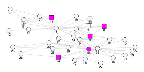
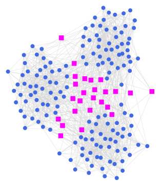
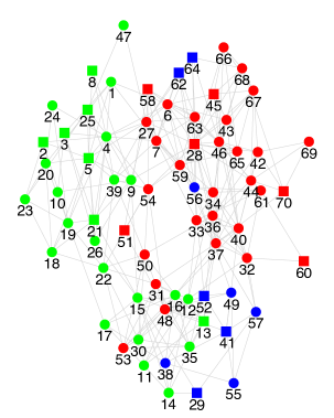
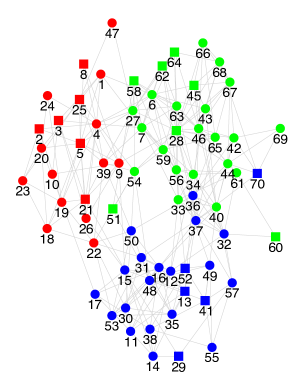
(a) Zachary’s karate club network. Highlighted nodes in magenta are the actual sites of excitations, while nodes marked as rectangles are the detected sites of excitations using boosted BlindCD. The only mismatches were node ‘4’ and ‘34’.

(b) BlindCD result	(c) Boosted BlindCD result

Figure 3: Experiments on Zachary’s karate club network. The network consists of $N=34$ nodes and (approximately) $K=2$ communities. The graph filter models a diffusion dynamics with an order of $T_{\sf d}=6$ and the graph signals observed have only rank $R=5$ as only $5$ nodes are injected with input signals. The bottom plots show the result of both BlindCD methods.

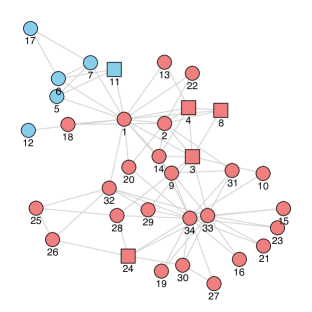
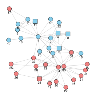
The example in Fig. 3 shows the performance of an instance of BlindCD on the Zachary’s Karate Club network when the graph signals are generated from the diffusion dynamics. To capitalize on the benefit of the boosting technique, we consider a scenario with a filter order of $T_{\sf d}=6$, observation rank of $R=5$ (the graph is excited on just $5$ nodes) and we observe $L=10^{3}$ noisy samples of the graph signals. Observe that the low-pass coefficient for the filter may be close to $1$ as $T_{\sf d}$ is small. This explains the poorer performance of BlindCD in Fig. 3.(b). The boosted BlindCD, instead, delivers good performance as it identifies the two communities in the network except for a miss-classification of agent $17$. Through sorting the row sums of the estimated $\widehat{\bm{B}}$, we also detected the sites of the excitations, as shown in the Fig. 3.a.

6.2 Network Dynamics Models

We describe applications of our BlindCD methods on detecting communities in consumer and social networks, where the models have been studied in Sections 3.2 and 3.3.

Figure 4: Snapshots of set-ups for case studies on network dynamics. (Left) A consumers network, where the highlighted nodes are the agents that the pricing experiments were performed on. (Right) A social network, where the highlighted nodes are the stubborn agents. Both networks are generated according to ${\sf SBM}(150,3,8\log N/N,\log N/(2N))$.

In the Monte-Carlo simulations below, we generate the graphs as $G\sim{\sf SBM}(150,3,8\log N/N,\log N/(2N))$, $N=150$. For the consumer games, ${\bm{A}}$ is taken as the binary adjacency matrix of $G$ and ${\bm{B}}$ is chosen as in (19) where the set of affected agents ${\mathcal{}I}$ is selected uniformly. Furthermore, in the utility (14), we set $b=2\|{\bm{A}}{\bf 1}\|_{\infty}$ and $a=2\max_{\ell}\|{\bm{p}}^{\ell}\|_{\infty}$ such that the equilibrium always satisfies (16). For the social networks, we first generate the support of ${\bm{B}}$ as a sparse bipartite graph with connectivity $2\log N/N$, then the weights on ${\bm{A}},{\bm{B}}$ are assigned uniformly such that all the rows in the concatenated matrix $[{\bm{A}},{\bm{B}}]$ sum up to one. This models a setting where the stubborn agents are connected sparsely to the others, i.e., they are located at the periphery of the communities. Note the support of ${\bm{A}}$ is symmetric with $A_{ij}\neq 0\Leftrightarrow A_{ji}\neq 0$. Snapshots of the set-ups for both networks are found in Fig. 4.

Despite the similarity to the previous examples, it is important to note that for the social networks, the Laplacian matrix ${\bm{L}}$ can be asymmetric. Nevertheless, we anticipate that BlindCD would work in this case provided that ${\bm{L}}$ is approximately symmetric. This symmetry in ${\bm{L}}$ is consistent with assuming that trust in social networks is of mutual nature.

The consumption levels and steady-state opinions can both be generated from the graph filter in Example 2. The difference between the two cases rests on the design of the sketch matrix ${\bm{B}}$. In the following, we fix the number of samples at $L=10^{4}$ with a noise variance of $\sigma_{w}^{2}=(10^{-1}/b^{2})^{2}$ for consumer games and $\sigma_{w}^{2}=10^{-2}$ for social networks. For the boosted BlindCD method, we set $\kappa=2/\sqrt{L},\rho=4/\sqrt{RL}$ for consumer games and $\kappa=2/\sqrt{L},\rho=1/\sqrt{RL}$ for social networks; and we test the formulation of (41) with the regularizer $g_{1}(\widehat{\bm{B}})$. For the social network, we included a comparison to a 2-step procedure which first recovers the graph topology using [22], and then applying spectral clustering on the inferred topology.

Figure 5: Community detection performance on cases of network dynamics. (Left) Pricing experiments on consumers network. (Right) Opinion dynamics with stubborn agents on social networks. In both cases, we consider networks generated as $G\sim{\sf SBM}(N,3,8\log N/N,\log N/(2N))$, $N=150$.

The results of our numerical experiments are shown in Fig. 5, where we compare the community detection performance as the excitation rank $R$ increases in both systems. Similar to the previous experiment in Fig. 2, for both cases we observe that the performance improves with $R$ and the boosted BlindCD method delivers the best performance consistently. Overall, the performance improvement with boosted BlindCD is greater than in the previous example [cf. Fig. 2]. The reason behind this is the fact that the IIR graph filter has a poor low-pass coefficient depending on the parameter $c\gg 1$ for the scenario we have considered. Another observation is that the community detection performance of the un-boosted BlindCD saturates at $R\approx 25$ for the opinion dynamics experiments while it continues to improve with $R$ for pricing ones. This is due to the different model used for the sketch matrix ${\bm{B}}$. In particular, for the pricing experiments, ${\bm{B}}$ is merely a sub-matrix of the identity matrix. Recall from Theorem 1 that the performance of BlindCD depend on the product $\|{\bm{V}}_{N-K}^{\top}{\bm{B}}{\bm{Q}}_{K}\|_{2}\|({\bm{V}}_{K}^{\top}{\bm{B}}{\bm{Q}}_{K})^{-1}\|_{2}$, which is anticipated to decrease since ${\bm{B}}$ approaches a permutation of ${\bm{I}}$ as $R$ approaches $N$, yielding a better performance. The same observation does not apply for opinion dynamics as the sketch matrix does not approximate the identity matrix as $R$ grows.

(a) Highschool network. The pricing experiments modify prices for the agents marked with square. The above clustering on the network is computed from the true Laplacian matrix ${\bm{L}}$, which has a RatioCut of $3.618$.

(b) BlindCD, RatioCut$=6.769$.	(c) Boosted BlindCD, RatioCut$=4.701$.

Figure 6: Pricing experiments on the Highschool network. The network comprises of $N=70$ agents and (approximately) $K=3$ communities. The utility parameters in (14) are $a=R$ and $b=2\|{\bm{A}}{\bf 1}\|_{\infty}$. The network’s equilibrium consumption levels are collected for $L=10^{3}$ samples, each observed with a noise variance of $\sigma_{w}^{2}=10^{-2}/b^{4}$. The pricing experiments are conducted through controlling the prices for $R=18$ agents.

(a) ReedCollege network. The clustering above is found by applying spectral clustering on the true ${\bm{L}}$. The obtained RatioCut is $0.1419$ w.r.t. ${\bm{A}}$.

(b) Applying BlindCD method. The obtained RatioCut is $0.8953$ w.r.t. ${\bm{A}}$.

(c) Applying Boosted BlindCD method. The obtained RatioCut is $0.5249$ w.r.t. ${\bm{A}}$.

Figure 7: Opinion dynamics experiments on ReedCollege network. The network comprises of $N=962$ agents and (approximately) $K=2$ communities. The network’s steady-state opinions are collected with $L=10^{4}$ samples, each observed with a noise variance of $\sigma_{w}^{2}=10^{-2}$. There are $R=150$ stubborn agents in the experiments, which are connected to the social network through a random bi-partite graph with connectivity $\log N/N$.

We then illustrate an application on real network topologies for the two network dynamics. Fig. 6 shows an example of simulated pricing experiments on the network highschool from [50], which is a friendship network between $N=70$ high school students with $|E|=273$ undirected edges. On the other hand, Fig. 7 shows the case study for opinion dynamics on the Facebook network of ReedCollege [51], which is a friendship network with $N=962$ college students with $|E|=18,812$ undirected edges, and we influence the network using $R=150$ stubborn agents. To handle the high dimensionality, we applied the fast algorithm from [52] to solve the robust PCA problem in (41). In both cases, we observe that the boosted BlindCD method recovers the communities in the networks, as evidenced from the illustrations and the ratio-cut scores.

6.3 Application to US Senate Rollcall Records

We consider applying the BlindCD methods to the US Senate rollcall record on https://voteview.com for the 110th congress. The dataset contains 657 rollcalls during the period from 2007 to 2009. To represent the opinions of the states during a rollcall, we consider the votes from the two Senators of a state by counting a ‘yay’ as 1, while a ‘nay’ or ‘absent’ is counted as 0. By treating each state as a node on a graph with $50$ nodes, this results in $L=657$ samples of graph signals with values $\{0,1,2\}$. As argued in [33], the rollcall data may be modeled as the equilibrium of an opinion dynamics process with stubborn agents. Therefore, we selected $4$ states – Massachusetts (MA), New York (NY), Alabama (AL), Louisiana (LA), which are the most liberal/conservative states [53], as the ‘stubborn’ states modeled in Section 3.3. We then apply the BlindCD methods to detect communities for the remaining $N=46$ states. For the boosted method, we use the sparse regularizer $g_{1}(\widehat{\bm{B}})$ to promote sparsity in the $\widehat{\bm{B}}^{\star}$ component of the solution.

Fig. 8 shows the $K=2$ communities detected using the proposed methods. We observe that the boosted BlindCD method successfully identifies Maine to be in the same community as Texas, where both states were controlled by Republicans in this congress. Fig. 9 shows the inferred $\widehat{\bm{B}}^{\star}$ matrix modeled in Section 3.3, where we labeled the rows as the stubborn states and the columns as the regular states. A large number in the table indicates strong influence from the stubborn to regular state. We observe consistent results, e.g., NY (resp. LA) positively influencing Illinois (resp. Arkansas) as both are Democrat (resp. Republican) states in this congress; NY is negatively influencing Idaho (Republican in this congress).

Figure 8: Applying BlindCD methods on the 110th US Senate Rollcall records. The states marked in red/blue are found to be in different communities; while the states marked in gray are marked as the ‘stubborn’ states as explained in the text. (Left) Results of BlindCD. (Right) Results of boosted BlindCD.

	CT	ME	NH	RI	VT	DE	NJ	PA	IL	IN	MI	OH	WI	IA	KS	MN
MA	0	0	0	9	4	0	0	8	0	0	0	5	0	0	0	0
NY	11	3	0	5	4	0	14	0	29	9	6	0	0	0	0	0
AL	0	0	31	0	0	0	0	0	0	0	0	0	0	5	5	0
LA	0	0	0	-2	0	0	0	0	0	2	13	0	0	0	0	0

	TN	WV	AZ	CO	ID	MT	NV	NM	UT	WY	CA	OR	WA	AK	HI
MA	2	8	0	4	6	0	0	0	2	0	0	6	0	0	0
NY	0	0	0	0	-9	0	0	0	0	0	10	0	0	0	0
AL	19	0	7	0	19	0	18	0	28	34	0	0	0	9	0
LA	0	5	0	0	0	28	0	0	0	0	0	0	0	0	0

	OK	MO	NE	ND	SD	VA	AR	FL	GA	MS	NC	SC	TX	KY	MD
MA	-7	6	0	0	1	0	1	0	0	-2	0	0	0	0	0
NY	0	0	0	0	0	0	0	8	0	0	0	0	0	0	8
AL	15	0	0	0	0	0	0	0	18	16	11	26	4	12	0
LA	0	19	11	20	2	0	34	5	0	5	0	0	5	0	0

Figure 9: Illustrating the $\widehat{\bm{B}}^{\star}$ matrix found with boosted BlindCD method [cf. (20),(41)]. Note that the values within the table have been rescaled.

7 Conclusions

This paper proposes two blind community detection methods for inferring community structure from graph signals. We consider a challenging and realistic setting where the observed graph signals are outcomes of a graph filter with low-rank excitations. The BlindCD methods rely on an intrinsic low-pass property of the graph filters that models the network dynamics. This property holds for common network processes and the accuracy of BlindCD is analyzed by viewing the graph signals as sketches of the graph filters. We propose a boosting technique to improve the performance of BlindCD. The technique leverages the latent ‘low-rank plus sparse’ structure related to the graph signals. Extensive numerical experiments verify our findings.

Appendix A Proof of Theorem 1

To simplify the notations while proving the theorem, let us define the following indicator matrices for the communities. Firstly, the matrix $\widehat{\bm{X}}\in\mathbb{R}^{N\times K}$ is associated with the communities $\{\hat{\mathcal{}C}_{1},...,\hat{\mathcal{}C}_{K}\}$ found with BlindCD and defined as

$$\hat{X}_{ij}\mathrel{\mathop{:}}=\begin{cases}{1/\sqrt{|\hat{\mathcal{}C}_{j}|}},&\text{if}~{}i\in\hat{\mathcal{}C}_{j},\\ 0,&\text{otherwise}.\end{cases}$$ (54)

We have

$$\|\widehat{\bm{V}}_{K}-\widehat{\bm{X}}\widehat{\bm{X}}^{\top}\widehat{\bm{V}}_{K}\|_{\rm F}^{2}=\sum_{k=1}^{K}\sum_{i\in\hat{\mathcal{}C}_{k}}\Big{\|}\hat{\bm{v}}_{i}^{\rm row}-\frac{1}{|\hat{\mathcal{}C}_{k}|}\sum_{j\in\hat{\mathcal{}C}_{k}}\hat{\bm{v}}_{j}^{\rm row}\Big{\|}_{2}^{2}.$$

Define ${\mathcal{}X}$ as the set of all possible indicator matrices of partitions. Using Condition 1 in Theorem 1, we have that

$$\begin{split}\|\widehat{\bm{V}}_{K}-\widehat{\bm{X}}\widehat{\bm{X}}^{\top}\widehat{\bm{V}}_{K}\|_{\rm F}^{2}&\leq(1+\epsilon)\min_{{\bm{X}}\in{\mathcal{}X}}\|\widehat{\bm{V}}_{K}-{\bm{X}}{\bm{X}}^{\top}\widehat{\bm{V}}_{K}\|_{\rm F}^{2}\\ &\leq(1+\epsilon)\|\widehat{\bm{V}}_{K}-{\bm{X}}^{\star}({\bm{X}}^{\star})^{\top}\widehat{\bm{V}}_{K}\|_{\rm F}^{2}\;,\\[-8.5359pt] \end{split}$$ (55)

where we have defined ${\bm{X}}^{\star}\in\mathbb{R}^{N\times K}$ by replacing $\hat{\mathcal{}C}_{i}$ in (54) with ${\mathcal{}C}_{i}^{\star}$ such that ${\mathcal{}C}_{1}^{\star},\ldots,{\mathcal{}C}_{K}^{\star}$ is an optimal set of communities found by minimizing $F({\mathcal{}C}_{1},...,{\mathcal{}C}_{K})$ [cf. (9)]. On the other hand, by the definition,

$$\begin{split}\|{\bm{V}}_{K}-{\bm{X}}^{\star}({\bm{X}}^{\star})^{\top}{\bm{V}}_{K}\|_{\rm F}^{2}&=\min_{{\bm{X}}\in{\mathcal{}X}}\|{\bm{V}}_{K}-{\bm{X}}{\bm{X}}^{\top}{\bm{V}}_{K}\|_{\rm F}^{2}\\ &=\min_{{\mathcal{}C}_{1},...,{\mathcal{}C}_{K}}F({\mathcal{}C}_{1},...,{\mathcal{}C}_{K})=F^{\star}\;,\vspace{-.4cm}\end{split}\vspace{.2cm}$$ (56)

and furthermore $\|{\bm{V}}_{K}-\widehat{\bm{X}}\widehat{\bm{X}}^{\top}{\bm{V}}_{K}\|_{\rm F}^{2}=F(\hat{\mathcal{}C}_{1},...,\hat{\mathcal{}C}_{K})$.

Define the error matrix as ${\bm{E}}\mathrel{\mathop{:}}={\bm{V}}_{K}{\bm{V}}_{K}^{\top}-\widehat{\bm{V}}_{K}\widehat{\bm{V}}_{K}^{\top}$. We observe the following chain of inequalities:

$$\begin{split}&\|{\bm{V}}_{K}-\widehat{\bm{X}}\widehat{\bm{X}}^{\top}{\bm{V}}_{K}\|_{\rm F}=\|({\bm{I}}-\widehat{\bm{X}}\widehat{\bm{X}}^{\top})(\widehat{\bm{V}}_{K}\widehat{\bm{V}}_{K}^{\top}+{\bm{E}})\|_{\rm F}\\ &\leq\|({\bm{I}}-\widehat{\bm{X}}\widehat{\bm{X}}^{\top})\widehat{\bm{V}}_{K}\widehat{\bm{V}}_{K}^{\top}\|_{\rm F}+\|({\bm{I}}-\widehat{\bm{X}}\widehat{\bm{X}}^{\top}){\bm{E}}\|_{\rm F}\\ &\leq\|({\bm{I}}-\widehat{\bm{X}}\widehat{\bm{X}}^{\top})\widehat{\bm{V}}_{K}\widehat{\bm{V}}_{K}^{\top}\|_{\rm F}+\|{\bm{E}}\|_{\rm F}\;,\\[-14.22636pt] \end{split}$$ (57)

where the first equality is due to ${\bm{V}}_{K}^{\top}{\bm{V}}_{K}={\bm{I}}$ and the last inequality is due to ${\bm{I}}-\widehat{\bm{X}}\widehat{\bm{X}}^{\top}$ is a projection matrix. Using (55), we have that

$$\begin{split}&\|({\bm{I}}-\widehat{\bm{X}}\widehat{\bm{X}}^{\top})\widehat{\bm{V}}_{K}\widehat{\bm{V}}_{K}^{\top}\|_{\rm F}+\|{\bm{E}}\|_{\rm F}\\ &\leq\sqrt{1+\epsilon}\|({\bm{I}}-{\bm{X}}^{\star}({\bm{X}}^{\star})^{\top})({\bm{V}}_{K}{\bm{V}}_{K}^{\top}-{\bm{E}})\|_{\rm F}+\|{\bm{E}}\|_{\rm F}\\ &\leq\sqrt{1+\epsilon}\|({\bm{I}}-{\bm{X}}^{\star}({\bm{X}}^{\star})^{\top}){\bm{V}}_{K}{\bm{V}}_{K}^{\top}\|_{\rm F}\\ &\hskip 28.45274pt+\sqrt{1+\epsilon}\|({\bm{I}}-{\bm{X}}^{\star}({\bm{X}}^{\star})^{\top}){\bm{E}}\|_{\rm F}+\|{\bm{E}}\|_{\rm F}\\ &\leq\sqrt{1+\epsilon}\|({\bm{I}}-{\bm{X}}^{\star}({\bm{X}}^{\star})^{\top}){\bm{V}}_{K}{\bm{V}}_{K}^{\top}\|_{\rm F}+(2+\epsilon)\|{\bm{E}}\|_{\rm F}\\ &=\sqrt{(1+\epsilon)F^{\star}}+(2+\epsilon)\|{\bm{E}}\|_{\rm F}\;,\end{split}$$ (58)

where we have used the fact ${\bm{I}}-{\bm{X}}^{\star}({\bm{X}}^{\star})^{\top}$ is a projection matrix and $\sqrt{1+\epsilon}\leq 1+\epsilon$ in the third inequality. The final step is to bound $\|{\bm{E}}\|_{\rm F}$, where we rely on the following results.

Lemma 4

[42, Lemma 7] For any ${\bm{A}},{\bm{B}}\in\mathbb{R}^{N\times K}$ with $N\geq K$ and ${\bm{A}}^{\top}{\bm{A}}={\bm{B}}^{\top}{\bm{B}}={\bm{I}}$, it holds that

$$\|{\bm{A}}{\bm{A}}^{\top}-{\bm{B}}{\bm{B}}^{\top}\|_{\rm F}^{2}\leq 2K\|{\bm{A}}{\bm{A}}^{\top}-{\bm{B}}{\bm{B}}^{\top}\|_{2}^{2}\;.\vspace{-.2cm}$$ (59)

Proposition 1

Under Conditions 2 to 4 in Theorem 1, we have

$$\|\overline{\bm{V}}_{K}\overline{\bm{V}}_{K}^{\top}-{\bm{V}}_{K}{\bm{V}}_{K}^{\top}\|_{2}^{2}=(1+\gamma^{2})^{-1}\gamma^{2}\;,$$ (60)

where the columns of $\overline{\bm{V}}_{K}$ are the top $K$ eigenvectors of $\overline{\bm{C}}_{y}$ and $\gamma$ is bounded as stated in (35).

Proposition 2

Under Condition 5 in Theorem 1, it holds that

$$\|\overline{\bm{V}}_{K}\overline{\bm{V}}_{K}^{\top}-\widehat{\bm{V}}_{K}\widehat{\bm{V}}_{K}^{\top}\|_{2}\leq\|\widehat{\bm{C}}_{y}-\overline{\bm{C}}_{y}\|_{2}/\delta\;.$$ (61)

The proofs of the propositions can be found in the subsections A and B of this appendix. Applying Lemma 4 we obtain that

$$\|{\bm{E}}\|_{\rm F}\leq\sqrt{2K}\|{\bm{V}}_{K}{\bm{V}}_{K}^{\top}-\widehat{\bm{V}}_{K}\widehat{\bm{V}}_{K}^{\top}\|_{2}\;.$$ (62)

Combining (60), (61) and using the triangle inequality yields

$$\begin{split}&\sqrt{F(\hat{\mathcal{}C}_{1},...,\hat{\mathcal{}C}_{K})}=\|({\bm{I}}-\widehat{\bm{X}}\widehat{\bm{X}}^{\top}){\bm{V}}_{K}{\bm{V}}_{K}^{\top}\|_{\rm F}\\ &\leq\sqrt{(1+\epsilon)F^{\star}}+(2+\epsilon)\sqrt{2K}\Big{(}\sqrt{\frac{\gamma^{2}}{1+\gamma^{2}}}+\frac{\|\widehat{\bm{C}}_{y}-\overline{\bm{C}}_{y}\|_{2}}{\delta}\Big{)},\end{split}$$

concluding the proof.

A.1 Proof of Proposition 1

We begin our proof by establishing the relationships between $\overline{\bm{V}}_{K},{\bm{V}}_{K}$ and the left singular vectors of ${\mathcal{}H}({\bm{L}}){\bm{B}}$. Denote the rank-$K$ approximation to ${\mathcal{}H}({\bm{L}})$ as $[{\mathcal{}H}({\bm{L}})]_{K}\mathrel{\mathop{:}}={\bm{V}}_{K}{\rm diag}(\tilde{\bm{h}}_{K}){\bm{V}}_{K}^{\top}$. This expression is valid due to the low pass property of ${\mathcal{}H}({\bm{L}})$. Define $\tilde{\bm{B}}\mathrel{\mathop{:}}={\bm{B}}{\bm{Q}}_{K}$, we observe that

$${\mathcal{}R}([{\mathcal{}H}({\bm{L}})]_{K})={\mathcal{}R}([{\mathcal{}H}({\bm{L}})]_{K}\tilde{\bm{B}})\;,$$ (63)

which is due to Condition 3 in Theorem 1 such that the linear transformation $\tilde{\bm{B}}$ does not modify the range space of $[{\mathcal{}H}({\bm{L}})]_{K}$. Similarly, $[\overline{\bm{C}}_{y}]_{K}\!\mathrel{\mathop{:}}=\!\overline{\bm{V}}_{K}{\rm diag}(\bm{\sigma}_{K})^{2}\overline{\bm{V}}_{K}^{\top}$ is the rank $K$ approximation to $\overline{\bm{C}}_{y}$. We observe the equivalences

$${\mathcal{}R}([\overline{\bm{C}}_{y}]_{K})={\mathcal{}R}([{\mathcal{}H}({\bm{L}}){\bm{B}}]_{K})={\mathcal{}R}({\mathcal{}H}({\bm{L}})\tilde{\bm{B}})$$ (64)

where the last equality is due to ${\mathcal{}H}({\bm{L}})\tilde{\bm{B}}={\mathcal{}H}({\bm{L}}){\bm{B}}{\bm{Q}}_{K}=\overline{\bm{V}}_{K}{\rm diag}(\bm{\sigma}_{K})$, as we recall that the columns of ${\bm{Q}}_{K}$ are the top $K$ right singular vectors of ${\mathcal{}H}({\bm{L}}){\bm{B}}$. Furthermore,

$${\mathcal{}R}([{\mathcal{}H}({\bm{L}})]_{K}\tilde{\bm{B}})~{}\bot~{}{\mathcal{}R}(({\mathcal{}H}({\bm{L}})-[{\mathcal{}H}({\bm{L}})]_{K})\tilde{\bm{B}})\;.$$ (65)

Let the columns of $\widetilde{\bm{V}}_{K}$ and $\widetilde{\overline{\bm{V}}}_{K}$ be respectively the top-$K$ singular vectors of $[{\mathcal{}H}({\bm{L}})]_{K}\tilde{\bm{B}}$ and ${\mathcal{}H}({\bm{L}})\tilde{\bm{B}}$, therefore (63) and (64) imply that ${\bm{V}}_{K}{\bm{V}}_{K}^{\top}=\widetilde{\bm{V}}_{K}\widetilde{\bm{V}}_{K}^{\top}$ and $\overline{\bm{V}}_{K}\overline{\bm{V}}_{K}^{\top}=\widetilde{\overline{\bm{V}}}_{K}\widetilde{\overline{\bm{V}}}_{K}^{\top}$. Invoking (65) with [54, Lemma 8] through setting ${\bf D}={\mathcal{}H}({\bm{L}})\tilde{\bm{B}}$, ${\bf C}=[{\mathcal{}H}({\bm{L}})]_{K}\tilde{\bm{B}}$ and ${\bf E}=({\mathcal{}H}({\bm{L}})-[{\mathcal{}H}({\bm{L}})]_{K})\tilde{\bm{B}}$ therein, and applying [55, Theorem 2.6.1], we obtain that

$$\begin{split}&\|{\bm{V}}_{K}{\bm{V}}_{K}^{\top}-\overline{\bm{V}}_{K}\overline{\bm{V}}_{K}^{\top}\|_{2}^{2}=\|\widetilde{\bm{V}}_{K}\widetilde{\bm{V}}_{K}^{\top}-\widetilde{\overline{\bm{V}}}_{K}\widetilde{\overline{\bm{V}}}_{K}^{\top}\|_{2}^{2}\\ &=1-\beta_{K}\Big{(}[{\mathcal{}H}({\bm{L}})]_{K}\tilde{\bm{B}}\bm{\Pi}^{\dagger}([{\mathcal{}H}({\bm{L}})]_{K}\tilde{\bm{B}})^{\top}\Big{)}\;,\end{split}$$ (66)

where we have defined $\bm{\Pi}\mathrel{\mathop{:}}=({\mathcal{}H}({\bm{L}})\tilde{\bm{B}})^{\top}{\mathcal{}H}({\bm{L}})\tilde{\bm{B}}$ and $\beta_{K}(\cdot)$ denotes the $K$th largest eigenvalue. Under Condition 4 in Theorem 1, the $K\times K$ matrix $\bm{\Pi}$ is non-singular. We observe the following chain of equalities

$$\begin{split}&\beta_{K}\Big{(}[{\mathcal{}H}({\bm{L}})]_{K}\tilde{\bm{B}}\bm{\Pi}^{-1}([{\mathcal{}H}({\bm{L}})]_{K}\tilde{\bm{B}})^{\top}\Big{)}\\ &=\beta_{K}\Big{(}{\rm diag}(\tilde{\bm{h}}_{K}){\bm{V}}_{K}^{\top}\tilde{\bm{B}}\bm{\Pi}^{-1}({\rm diag}(\tilde{\bm{h}}_{K}){\bm{V}}_{K}^{\top}\tilde{\bm{B}})^{\top}\Big{)}\\ &=\frac{1}{\beta_{1}\Big{(}({\rm diag}(\tilde{\bm{h}}_{K}){\bm{V}}_{K}^{\top}\tilde{\bm{B}})^{-\top}\bm{\Pi}({\rm diag}(\tilde{\bm{h}}_{K}){\bm{V}}_{K}^{\top}\tilde{\bm{B}})^{-1}\Big{)}}\;,\end{split}$$ (67)

where the first equality is due to $\beta_{K}({\bm{U}}{\bm{A}}{\bm{U}}^{\top})=\beta_{K}({\bm{A}})$ for any symmetric ${\bm{A}}$ and ${\bm{U}}\in\mathbb{R}^{N\times K}$ with orthogonal columns, and the second equality follows since the argument in $\beta_{K}(\cdot)$ is of rank $K$. Moreover, $\bm{\Pi}$ admits the decomposition

$$\begin{split}\bm{\Pi}&=({\mathcal{}H}({\bm{L}})\tilde{\bm{B}})^{\top}{\mathcal{}H}({\bm{L}})\tilde{\bm{B}}=\tilde{\bm{B}}^{\top}{\mathcal{}H}({\bm{L}})^{\top}{\mathcal{}H}({\bm{L}})\tilde{\bm{B}}\\ &=\tilde{\bm{B}}^{\top}{\bm{V}}_{K}{\rm diag}(\tilde{\bm{h}}_{K})^{2}{\bm{V}}_{K}^{\top}\tilde{\bm{B}}\\ &\hskip 14.22636pt+\tilde{\bm{B}}^{\top}{\bm{V}}_{N-K}{\rm diag}(\tilde{\bm{h}}_{N-K})^{2}{\bm{V}}_{N-K}^{\top}\tilde{\bm{B}}\;.\end{split}$$ (68)

Thus, yielding that

$$\begin{split}&\beta_{K}\Big{(}[{\mathcal{}H}({\bm{L}})]_{K}\tilde{\bm{B}}\bm{\Pi}^{-1}([{\mathcal{}H}({\bm{L}})]_{K}\tilde{\bm{B}})^{\top}\Big{)}\\ &=\Big{(}1+\beta_{1}\Big{(}({\rm diag}(\tilde{\bm{h}}_{K}){\bm{V}}_{K}^{\top}\tilde{\bm{B}})^{-\top}\tilde{\bm{B}}^{\top}{\bm{V}}_{N-K}\\ &\hskip 28.45274pt{\rm diag}(\tilde{\bm{h}}_{N-K})^{2}{\bm{V}}_{N-K}^{\top}\tilde{\bm{B}}({\rm diag}(\tilde{\bm{h}}_{K}){\bm{V}}_{K}^{\top}\tilde{\bm{B}})^{-1}\Big{)}\Big{)}^{-1}\\ &=\frac{1}{1+\|{\rm diag}(\tilde{\bm{h}}_{N-K}){\bm{V}}_{N-K}^{\top}\tilde{\bm{B}}({\rm diag}(\tilde{\bm{h}}_{K}){\bm{V}}_{K}^{\top}\tilde{\bm{B}})^{-1}\|_{2}^{2}}\\ &=\Big{(}1+\gamma^{2}\Big{)}^{-1}\;,\end{split}$$

where we have defined $\gamma$ such that

$$\begin{split}\gamma&\mathrel{\mathop{:}}=\|{\rm diag}(\tilde{\bm{h}}_{N-K}){\bm{V}}_{N-K}^{\top}\tilde{\bm{B}}({\rm diag}(\tilde{\bm{h}}_{K}){\bm{V}}_{K}^{\top}\tilde{\bm{B}})^{-1}\|_{2}\\ &\leq\eta\!~{}\|{\bm{V}}_{N-K}^{\top}{\bm{B}}{\bm{Q}}_{K}\|_{2}\|({\bm{V}}_{K}^{\top}{\bm{B}}{\bm{Q}}_{K})^{-1}\|_{2}\;.\end{split}$$ (69)

Substituting the above into (66) concludes the proof.

A.2 Proof of Proposition 2

Denote the SVD of the sampled covariance as $\widehat{\bm{C}}_{y}=\widehat{\bm{V}}\widehat{\bm{\Sigma}}\widehat{\bm{V}}^{\top}$. The left hand side of (61) can be written as

$$\|\overline{\bm{V}}_{K}\overline{\bm{V}}_{K}^{\top}-\widehat{\bm{V}}_{K}\widehat{\bm{V}}_{K}^{\top}\|_{2}=\|\widehat{\bm{V}}_{N-K}^{\top}\overline{\bm{V}}_{K}\|_{2}\;,$$ (70)

where the equality is due to [55, Theorem 2.6.1].

Define $\bm{\Delta}\mathrel{\mathop{:}}=\widehat{\bm{C}}_{y}-\overline{\bm{C}}_{y}$. Condition 5 in Theorem 1 implies that the largest eigenvalue in $\hat{\bm{\Sigma}}_{N-K}$ will never exceed $\beta_{K}(\overline{\bm{C}}_{y})-\delta$ since

$$\begin{split}\beta_{\sf max}(\hat{\bm{\Sigma}}_{N-K})=\beta_{K+1}(\widehat{\bm{C}}_{y})&\leq\beta_{K+1}(\overline{\bm{C}}_{y})+\beta_{1}(\bm{\Delta})\\ &\leq\beta_{K+1}(\overline{\bm{C}}_{y})+\|\bm{\Delta}\|_{2}\;,\end{split}$$ (71)

where the first inequality is due to Weyl’s inequality [55]. The perturbed matrix $\widehat{\bm{C}}_{y}$ thus satisfies the requirement of the Davis-Kahan’s $\sin(\Theta)$ theorem [56]

$$\|\widehat{\bm{V}}_{N-K}^{\top}\overline{\bm{V}}_{K}\|_{2}\leq\delta^{-1}\|\widehat{\bm{V}}_{N-K}^{\top}\bm{\Delta}\overline{\bm{V}}_{K}\|_{2}\;.$$ (72)

The inequality in (61) is obtained by observing that both $\overline{\bm{V}}_{K}$ and $\widehat{\bm{V}}_{N-K}$ are orthogonal matrices.

Appendix B Proof of Lemma 2

Fix $1\geq c>0$. Under the conditions stated in the lemma, the least-squares optimization (37) admits a closed form solution

$$\bm{\mathcal{H}}^{\star}-{\mathcal{}H}({\bm{L}}){\bm{B}}=\Big{(}\sum_{\ell=1}^{L}{\bm{w}}^{\ell}({\bm{z}}^{\ell})^{\top}\Big{)}\Big{(}\sum_{\ell=1}^{L}{\bm{z}}^{\ell}({\bm{z}}^{\ell})^{\top}\Big{)}^{-1},$$ (73)

where ${\bm{w}}^{\ell}$ was introduced in (11). Denoting the right hand side in (73) by $\bm{\mathcal{E}}$, we have that

$$\begin{split}\|\bm{\mathcal{E}}\|_{2}&=\left\|\Big{(}\frac{1}{L}\sum_{\ell=1}^{L}{\bm{w}}^{\ell}({\bm{z}}^{\ell})^{\top}\Big{)}\Big{(}\frac{1}{L}\sum_{\ell=1}^{L}{\bm{z}}^{\ell}({\bm{z}}^{\ell})^{\top}\Big{)}^{-1}\right\|_{2}\\ &\leq\left\|\frac{1}{L}\sum_{\ell=1}^{L}{\bm{w}}^{\ell}({\bm{z}}^{\ell})^{\top}\right\|_{2}\left\|\Big{(}\frac{1}{L}\sum_{\ell=1}^{L}{\bm{z}}^{\ell}({\bm{z}}^{\ell})^{\top}\Big{)}^{-1}\right\|_{2}.\end{split}$$ (74)

Observe that $\frac{1}{L}\sum_{\ell=1}^{L}{\bm{z}}^{\ell}({\bm{z}}^{\ell})^{\top}$ converges to ${\bm{I}}$ such that with probability at least $1-c$,

$$\left\|\frac{1}{L}\sum_{\ell=1}^{L}{\bm{z}}^{\ell}({\bm{z}}^{\ell})^{\top}-{\bm{I}}\right\|_{2}\leq C_{0}\!~{}\sqrt{\frac{R\log(1/c)}{L}}\;,$$ (75)

for some constant $C_{0}$. Applying [57, Proposition 2.1] we get that

$$\begin{split}\left\|\Big{(}\frac{1}{L}\sum_{\ell=1}^{L}{\bm{z}}^{\ell}({\bm{z}}^{\ell})^{\top}\Big{)}^{-1}\right\|_{2}&\leq\left(1-\Big{\|}\frac{1}{L}\sum_{\ell=1}^{L}{\bm{z}}^{\ell}({\bm{z}}^{\ell})^{\top}-{\bm{I}}\Big{\|}_{2}\right)^{-1}\\ &\leq\left(1-C_{0}\!~{}\sqrt{\frac{R\log(1/c)}{L}}\right)^{-1}.\end{split}$$

On the other hand, observe that $\mathbb{E}[{\bm{w}}^{\ell}({\bm{z}}^{\ell})^{\top}]=0$ and $\|{\bm{w}}^{\ell}({\bm{z}}^{\ell})^{\top}\|\leq C_{w}$ almost surely. Applying the matrix Bernstein’s inequality [58, Theorem 1.6] shows that with probability at least $1-c$ and for sufficiently large $L$,

$$\left\|\frac{1}{L}\sum_{\ell=1}^{L}{\bm{w}}^{\ell}({\bm{z}}^{\ell})^{\top}\right\|_{2}\leq C_{1}\!~{}\sqrt{\frac{\sigma_{w}^{2}\log((N+R)/c)}{L}}\;,$$ (76)

for some constant $C_{1}$. Finally, with probability at least $1-2c$,

$$\|\bm{\mathcal{E}}\|_{2}\leq\frac{C_{1}\sqrt{\sigma_{w}^{2}\log((N+R)/c)}}{\sqrt{L}-C_{0}\sqrt{R\log(1/c)}}={\mathcal{}O}(\sigma_{w}/\sqrt{L})\;.\vspace{-.1cm}$$ (77)

Appendix C Proof of Corollary 1

Let $\widetilde{\bm{V}}_{K}$ and $\widetilde{\bm{S}}_{K}$ be the top $K$ left singular vectors of $\widetilde{\mathcal{}H}({\bm{L}}){\bm{B}}$ and $\widehat{\bm{\mathcal{S}}}^{\star}$, respectively. We can repeat the proof for Theorem 1 up to (58) by re-defining the error matrix ${\bm{E}}$ therein as $\widetilde{\bm{E}}={\bm{V}}_{K}{\bm{V}}_{K}^{\top}-\widetilde{\bm{S}}_{K}\widetilde{\bm{S}}_{K}^{\top}$. This entails

$$\sqrt{F(\tilde{\mathcal{}C}_{1},...,\tilde{\mathcal{}C}_{K})}-\sqrt{(1+\epsilon)F^{\star}}\leq(2+\epsilon)\|\widetilde{\bm{E}}\|_{\rm F}\;.$$ (78)

Next, we bound $\|\widetilde{\bm{E}}\|_{\rm F}$. Applying Lemma 4 and using the triangle inequality we get that

$$\begin{split}\|\widetilde{\bm{E}}\|_{\rm F}&\leq\sqrt{2K}\|{\bm{V}}_{K}{\bm{V}}_{K}^{\top}-\widetilde{\bm{S}}_{K}\widetilde{\bm{S}}_{K}^{\top}\|_{2}\\ &\leq\sqrt{2K}\big{(}\|{\bm{V}}_{K}{\bm{V}}_{K}^{\top}-\widetilde{\bm{V}}_{K}\widetilde{\bm{V}}_{K}^{\top}\|_{2}+\|\widetilde{\bm{V}}_{K}\widetilde{\bm{V}}_{K}^{\top}-\widetilde{\bm{S}}_{K}\widetilde{\bm{S}}_{K}^{\top}\|_{2}\big{)},\end{split}$$

Proposition 1 implies that

$$\|{\bm{V}}_{K}{\bm{V}}_{K}^{\top}-\widetilde{\bm{V}}_{K}\widetilde{\bm{V}}_{K}^{\top}\|_{2}\leq\sqrt{\tilde{\gamma}/(1+\tilde{\gamma})},$$ (79)

where $\tilde{\gamma}$ is bounded as in (51). Our remaining task is to bound $\|\widetilde{\bm{V}}_{K}\widetilde{\bm{V}}_{K}^{\top}-\widetilde{\bm{S}}_{K}\widetilde{\bm{S}}_{K}^{\top}\|_{2}$. Observe that

$$\|\widetilde{\bm{V}}_{K}\widetilde{\bm{V}}_{K}^{\top}-\widetilde{\bm{S}}_{K}\widetilde{\bm{S}}_{K}^{\top}\|_{2}=\|\widetilde{\bm{S}}_{R-K}^{\top}\widetilde{\bm{V}}_{K}\|_{2}$$ (80)

and

$$\sigma_{K}(\widehat{\bm{\mathcal{S}}}^{\star})\geq\sigma_{K}(\widetilde{\mathcal{}H}({\bm{L}}){\bm{B}})-\|\widetilde{\bm{\Delta}}\|_{2}\;,$$ (81)

where we recalled the definition $\widetilde{\bm{\Delta}}=\widehat{\bm{\mathcal{S}}}^{\star}-\widetilde{\mathcal{}H}({\bm{L}}){\bm{B}}$ and applied the Weyl’s inequality [55]. From (49), we have that

$$\sigma_{K}(\widetilde{\mathcal{}H}({\bm{L}}){\bm{B}})-\|\widetilde{\bm{\Delta}}\|_{2}=\sigma_{K+1}(\widetilde{\mathcal{}H}({\bm{L}}){\bm{B}})+\tilde{\delta}\;,$$ (82)

with $\tilde{\delta}>0$. Finally, applying the Wedin theorem [59] yields

$$\|\widetilde{\bm{S}}_{R-K}^{\top}\widetilde{\bm{V}}_{K}\|_{2}\leq(\tilde{\delta})^{-1}\!~{}\|\widetilde{\bm{\Delta}}\|_{2}\;.$$ (83)

References

- [1] A. Sandryhaila and J. M. Moura, “Discrete signal processing on graphs,” IEEE Trans. Signal Process., vol. 61, no. 7, pp. 1644–1656, 2013.
- [2] D. Shuman, S. Narang, P. Frossard, A. Ortega, and P. Vandergheynst, “The emerging field of signal processing on graphs: Extending high-dimensional data analysis to networks and other irregular domains,” IEEE Signal Process. Mag., vol. 30, no. 3, pp. 83–98, May 2013.
- [3] A. Ortega, P. Frossard, J. Kovačević, J. M. Moura, and P. Vandergheynst, “Graph signal processing,” arXiv preprint arXiv:1712.00468, 2017.
- [4] A. G. Marques, S. Segarra, G. Leus, and A. Ribeiro, “Sampling of graph signals with successive local aggregations,” IEEE Trans. Signal Process., vol. 64, no. 7, pp. 1832–1843, April 2016.
- [5] S. Chen, R. Varma, A. Sandryhaila, and J. Kovačević, “Discrete signal processing on graphs: Sampling theory,” IEEE Trans. Signal Process., vol. 63, no. 24, pp. 6510–6523, Dec 2015.
- [6] D. Romero, M. Ma, and G. B. Giannakis, “Kernel-based reconstruction of graph signals,” IEEE Trans. Signal Process., vol. 65, no. 3, pp. 764–778, Feb 2017.
- [7] S. Segarra, A. G. Marques, G. Leus, and A. Ribeiro, “Reconstruction of graph signals through percolation from seeding nodes,” IEEE Trans. Signal Process., vol. 64, no. 16, pp. 4363–4378, Aug 2016.
- [8] S. Segarra, A. G. Marques, and A. Ribeiro, “Optimal graph-filter design and applications to distributed linear network operators,” IEEE Trans. Signal Process., vol. 65, no. 15, pp. 4117–4131, Aug 2017.
- [9] E. Isufi, A. Loukas, A. Simonetto, and G. Leus, “Autoregressive moving average graph filtering,” IEEE Trans. Signal Process., vol. 65, no. 2, pp. 274–288, Jan 2017.
- [10] J. Friedman, T. Hastie, and R. Tibshirani, “Sparse inverse covariance estimation with the graphical lasso,” Biostatistics, vol. 9, no. 3, pp. 432–441, 2008.
- [11] E. Pavez and A. Ortega, “Generalized Laplacian precision matrix estimation for graph signal processing,” in IEEE Intl. Conf. Acoust., Speech and Signal Process. (ICASSP), Shanghai, China, Mar. 20-25, 2016.
- [12] Y. Shen, B. Baingana, and G. B. Giannakis, “Kernel-based structural equation models for topology identification of directed networks,” IEEE Trans. Signal Process., vol. 65, no. 10, pp. 2503–2516, 2017.
- [13] X. Cai, J. A. Bazerque, and G. B. Giannakis, “Sparse structural equation modeling for inference of gene regulatory networks exploiting genetic perturbations,” PLoS, Computational Biology, Jun. 2013.
- [14] H.-T. Wai, A. Scaglione, U. Harush, B. Barzel, and A. Leshem, “Rids: Robust identification of sparse gene regulatory networks from perturbation experiments,” arXiv preprint arXiv:1612.06565, 2016.
- [15] X. Dong, D. Thanou, P. Frossard, and P. Vandergheynst, “Learning Laplacian matrix in smooth graph signal representations,” IEEE Trans. Signal Process., vol. 64, no. 23, pp. 6160–6173, Dec 2016.
- [16] V. Kalofolias, “How to learn a graph from smooth signals,” in Intl. Conf. Artif. Intel. Stat. (AISTATS). J Mach. Learn. Res., 2016, pp. 920–929.
- [17] S. P. Chepuri, S. Liu, G. Leus, and A. O. Hero, “Learning sparse graphs under smoothness prior,” in IEEE Intl. Conf. Acoust., Speech and Signal Process. (ICASSP), March 2017, pp. 6508–6512.
- [18] S. Segarra, A. G. Marques, G. Mateos, and A. Ribeiro, “Network topology inference from spectral templates,” IEEE Trans. Signal and Info. Process. over Networks, vol. 3, no. 3, pp. 467–483, 2017.
- [19] S. Segarra, G. Mateos, A. G. Marques, and A. Ribeiro, “Blind identification of graph filters,” IEEE Trans. Signal Process., vol. 65, no. 5, pp. 1146–1159, March 2017.
- [20] R. Shafipour, S. Segarra, A. G. Marques, and G. Mateos, “Network topology inference from non-stationary graph signals,” in Proc. ICASSP, March 2017, pp. 5870–5874.
- [21] H. E. Egilmez, E. Pavez, and A. Ortega, “Graph learning from filtered signals: Graph system and diffusion kernel identification,” IEEE Transactions on Signal and Information Processing over Networks, 2018.
- [22] H.-T. Wai, A. Scaglione, and A. Leshem, “Active sensing of social networks,” IEEE Trans. Signal and Info. Process. over Networks, vol. 2, no. 3, pp. 406–419, 2016.
- [23] D. Marbach, J. C. Costello, R. Küffner, N. M. Vega, R. J. Prill, D. M. Camacho, K. R. Allison, A. Aderhold, R. Bonneau, Y. Chen et al., “Wisdom of crowds for robust gene network inference,” Nature methods, vol. 9, no. 8, p. 796, 2012.
- [24] S. Fortunato, “Community detection in graphs,” Physics reports, vol. 486, no. 3, pp. 75–174, 2010.
- [25] O. Candogan, K. Bimpikis, and A. Ozdaglar, “Optimal pricing in networks with externalities,” Operations Research, vol. 60, no. 4, pp. 883–905, 2012.
- [26] B. Ata, A. Belloni, and O. Candogan, “Latent agents in networks: Estimation and pricing,” arXiv:1808.04878v1, August 2018.
- [27] M. H. DeGroot, “Reaching a consensus,” Journal of the American Statistical Association, vol. 69, no. 345, pp. 118–121, 1974.
- [28] H. Zha, X. He, C. Ding, M. Gu, and H. D. Simon, “Spectral relaxation for k-means clustering,” in Advances in neural information processing systems, 2002, pp. 1057–1064.
- [29] E. Abbe, “Community detection and stochastic block models: recent developments,” The Journal of Machine Learning Research, vol. 18, no. 1, pp. 6446–6531, 2017.
- [30] U. von Luxburg, “A tutorial on spectral clustering,” Statistics and Computing, vol. 17, no. 4, pp. 395–416, Dec 2007.
- [31] J. A. Hartigan and M. A. Wong, “Algorithm AS 136: A k-means clustering algorithm,” Journal of the Royal Statistical Society. Series C (Applied Statistics), vol. 28, no. 1, pp. 100–108, 1979.
- [32] A. Kumar, Y. Sabharwal, and S. Sen, “A simple linear time (1+)-approximation algorithm for k-means clustering in any dimensions,” in FOCS. IEEE, 2004, pp. 454–462.
- [33] S. X. Wu, H.-T. Wai, and A. Scaglione, “Estimating social opinion dynamics models from voting records,” IEEE Transactions on Signal Processing, vol. 66, no. 16, pp. 4193–4206, 2018.
- [34] D. Acemoglu, A. Ozdaglar, and A. ParandehGheibi, “Spread of (mis) information in social networks,” Games and Economic Behavior, vol. 70, no. 2, pp. 194–227, 2010.
- [35] E. Yildiz, A. Ozdaglar, D. Acemoglu, A. Saberi, and A. Scaglione, “Binary opinion dynamics with stubborn agents,” ACM Transactions on Economics and Computation (TEAC), vol. 1, no. 4, p. 19, 2013.
- [36] P. Jia, A. MirTabatabaei, N. E. Friedkin, and F. Bullo, “Opinion dynamics and the evolution of social power in influence networks,” SIAM review, vol. 57, no. 3, pp. 367–397, 2015.
- [37] M. E. Yildiz and A. Scaglione, “Computing along routes via gossiping,” IEEE Trans. on Signal Process., vol. 58, no. 6, pp. 3313–3327, 2010.
- [38] A. Ben-Tal and A. Nemirovski, Lectures on modern convex optimization: analysis, algorithms, and engineering applications. Siam, 2001, vol. 2.
- [39] R. Shafipour, A. Hashemi, G. Mateos, and H. Vikalo, “Online topology inference from streaming stationary graph signals,” submitted to DSW 2019, 2019.
- [40] J. Tsitsiklis, “Problems in decentralized decision making and computation,” Ph.D. dissertation, Dept. of Electrical Engineering and Computer Science, M.I.T., Boston, MA, 1984.
- [41] D. P. Bertsekas, Nonlinear programming. Athena scientific Belmont, 1999.
- [42] C. Boutsidis, P. Kambadur, and A. Gittens, “Spectral clustering via the power method-provably,” in International Conference on Machine Learning, 2015, pp. 40–48.
- [43] N. Tremblay, G. Puy, R. Gribonval, and P. Vandergheynst, “Compressive spectral clustering,” in International Conference on Machine Learning, 2016, pp. 1002–1011.
- [44] R. Vershynin, High-Dimensional Probability. Cambridge University Press, 2017.
- [45] A. Agarwal, S. Negahban, and M. J. Wainwright, “Noisy matrix decomposition via convex relaxation: Optimal rates in high dimensions,” The Annals of Statistics, pp. 1171–1197, 2012.
- [46] J. Huang, T. Zhang, and D. Metaxas, “Learning with structured sparsity,” JMLR, vol. 12, no. Nov, pp. 3371–3412, 2011.
- [47] S. N. Negahban, P. Ravikumar, M. J. Wainwright, and B. Yu, “A unified framework for high-dimensional analysis of m-estimators with decomposable regularizers,” Statistical Science, pp. 538–557, 2012.
- [48] P. W. Holland, K. B. Laskey, and S. Leinhardt, “Stochastic blockmodels: First steps,” Social networks, vol. 5, no. 2, pp. 109–137, 1983.
- [49] F. D. Malliaros and M. Vazirgiannis, “Clustering and community detection in directed networks: A survey,” Physics Reports, vol. 533, no. 4, pp. 95–142, 2013.
- [50] J. S. Coleman et al., “Introduction to mathematical sociology.” Introduction to mathematical sociology., 1964.
- [51] A. L. Traud, P. J. Mucha, and M. A. Porter, “Social structure of Facebook networks,” Physica A: Statistical Mechanics and its Applications, vol. 391, no. 16, pp. 4165–4180, 2012.
- [52] A. Aravkin, S. Becker, V. Cevher, and P. Olsen, “A variational approach to stable principal component pursuit,” in UAI, July 2014.
- [53] P. R. Center, “Political ideology by state.” [Online]. Available: http://www.pewforum.org/religious-landscape-study/compare/political-ideology/by/state/
- [54] A. Gittens, P. Kambadur, and C. Boutsidis, “Approximate spectral clustering via randomized sketching,” arXiv:1311.2854v1, 2013.
- [55] G. H. Golub and C. F. Van Loan, Matrix computations. JHU Press, 2012, vol. 3.
- [56] C. Davis and W. M. Kahan, “The rotation of eigenvectors by a perturbation. iii,” SIAM Journal on Numerical Analysis, vol. 7, no. 1, pp. 1–46, 1970.
- [57] R. Vershynin, “How close is the sample covariance matrix to the actual covariance matrix?” Journal of Theoretical Probability, vol. 25, no. 3, pp. 655–686, 2012.
- [58] J. A. Tropp, “User-friendly tail bounds for sums of random matrices,” Foundations of computational mathematics, vol. 12, no. 4, pp. 389–434, 2012.
- [59] P.-A. Wedin, “Perturbation bounds in connection with singular value decomposition,” BIT Numerical Mathematics, vol. 12, no. 1, pp. 99–111, 1972.