Differences in water vapor radiative transfer among 1D models can significantly affect the inner edge of the habitable zone

Abstract

An accurate estimate of the inner edge of the habitable zone is critical for determining which exoplanets are potentially habitable and for designing future telescopes to observe them. Here, we explore differences in estimating the inner edge among seven one-dimensional (1D) radiative transfer models: two line-by-line codes (SMART and LBLRTM) as well as five band codes (CAM3, CAM4_Wolf, LMDG, SBDART, and AM2) that are currently being used in global climate models. We compare radiative fluxes and spectra in clear-sky conditions around G- and M-stars, with fixed moist adiabatic profiles for surface temperatures from 250 to 360 K. We find that divergences among the models arise mainly from large uncertainties in water vapor absorption in the window region (10 $\mu$m) and in the region between 0.2 and 1.5 $\mu$m. Differences in outgoing longwave radiation increase with surface temperature and reach 10-20 W m^-2; differences in shortwave reach up to 60 W m^-2, especially at the surface and in the troposphere, and are larger for an M-dwarf spectrum than a solar spectrum. Differences between the two line-by-line models are significant, although smaller than among the band models. Our results imply that the uncertainty in estimating the insolation threshold of the inner edge (the runaway greenhouse limit) due only to clear-sky radiative transfer is $\approx$ 10 % of modern Earth’s solar constant (i.e., $\approx$ 34 W m^-2 in global mean) among band models and $\approx$ 3 % between the two line-by-line models. These comparisons show that future work is needed focusing on improving water vapor absorption coefficients in both shortwave and longwave, as well as on increasing the resolution of stellar spectra in broadband models.

1 Introduction

About 1600 planets orbiting other stars have been confirmed, and their number is constantly rising. A critical question is which of these planets are potentially habitable. Because liquid water is necessary for all known life on Earth, potentially habitable planets are generally defined as planets in the region around a star where they can maintain liquid water on their surface (Kasting, 2010). This region is called the habitable zone (Kasting et al., 1993, 2014). A standard assumption for the habitable zone is that the atmosphere is mainly composed of H₂O, CO₂, and N₂. Another critical assumption is that the silicate-weathering feedback functions on exoplanets. This feedback has been proposed based on studies of Earth’s history and would regulate CO₂ through the dependence of CO₂ removal by silicate weathering on planetary surface temperature and precipitation (Walker et al., 1981). If the the silicate-weathering feedback is functioning, the atmospheric CO₂ concentration should be low for planets near the inner edge of the habitable zone and high for planets near the outer edge of the habitable zone.

In this study, we focus on the inner edge of the habitable zone, which is determined by the loss of surface liquid water through either a moist greenhouse state or a runaway greenhouse state (Kasting, 1988; Nakajima et al., 1992; Abe, 1993). The purpose of this study is to calculate the inner edge of the habitable zone (in particular the runaway greenhouse limit) using seven 1D, cloud-free radiative transfer models, and to compare the differences among the models.

For both moist and runaway greenhouse states, the key process is the water vapor feedback: As the stellar flux increases, surface and atmospheric temperatures increase; the saturation water vapor pressure increases approximately exponentially with temperature following the Clausius–Clapeyron relation; and the increased atmospheric water vapor further warms the surface and the atmosphere because water vapor is a strong greenhouse gas and a good shortwave absorber. Once the mixing ratio of water vapor in the stratosphere becomes very high, the loss of water to space via photolysis and hydrogen escape will be significant. This process is called the moist greenhouse. For instance, if the stratospheric water vapor volume mixing ratio exceeds $\approx$ 3$\times$10^-3, Earth would lose an entire ocean’s worth of water (1.3 $\times$ 10¹⁸ m³) over the age of the Solar system ($\approx$ 4.6 billion years, Kasting, 1988).

The runaway greenhouse state arises from an energy imbalance, in which the atmosphere becomes optically thick in all infrared wavelengths, and absorbed stellar flux exceeds thermal infrared emission (Pierrehumbert, 2010; Goldblatt & Watson, 2012). In the runaway greenhouse, a planet will keep warming until all surface liquid water evaporates. During a runaway greenhouse the stratosphere typically becomes moist and water escapes rapidly to space. A third, empirical limit of the inner edge of the habitable zone has also been defined based on the fact that Venus may have had liquid water on its surface until about one billion years ago (Kasting et al., 1993), although this limit may depend on planetary rotation rate (Yang et al., 2014).

The inner edge of the habitable zone was estimated using a 1D climate model by Kasting et al. (1993) and Abe (1993), and recently this work was updated by Kopparapu et al. (2013, 2014) and Kasting et al. (2014). Using a 1D model and assuming a cloud-free and saturated atmosphere, Kopparapu et al. (2014) computed the inner edge of the habitable zone around the present Sun to be 0.99, 0.97, and 0.75 AU for the moist greenhouse limit, the runaway greenhouse limit, and the recent Venus limit, respectively. The corresponding solar fluxes are 1380, 1420, and 2414 W m^-2, respectively, which can be compared to Earth’s present-day solar flux of about 1360 W m^-2. For K and M stars, the insolation threshold of the inner edge is smaller due to the fact that a redder stellar spectrum causes a lower planetary albedo. Meanwhile, K and M stars are cooler and smaller than the Sun, so that the inner edge is located much closer to the host star. For F stars, the conditions are opposite to those of K and M stars, so that the insolation threshold is larger, and the habitable zone is farther away from the host star (Kasting et al., 1993). Apart from the stellar spectrum, other factors can also influence the insolation threshold, for example planetary gravity (Pierrehumbert, 2010; Kopparapu et al., 2014) and background gas concentrations (such as N₂; Goldblatt et al. (2013)). Furthermore, the inner edge of the habitable zone of dry planets (desert worlds with limited surface water) may be much closer to the host stars (Abe et al., 2011; Kodama et al., 2015).

Besides the work of Kasting et al. (1993) and Kopparapu et al. (2013), other 1D radiative transfer models have also been employed to estimate the inner edge of the habitable zone. The inter-model differences are significant and the predicted insolation thresholds for the runaway greenhouse limit vary by up to $\approx$ 80 W m^-2 (i.e., 20 W m^-2 of radiation impinging on the planet after geometric factors are accounted for). Using SMART, Goldblatt et al. (2013) found that the insolation threshold of the inner edge for a pure vapor atmosphere is $\approx$ 1340 W m^-2. In contrast, Kopparapu et al. (2013) and Leconte et al. (2013) found a threshold of $\approx$ 1420 W m^-2 in Kasting’s radiative transfer model and in the 1D model LMDG, even though all groups used the same surface albedo of 0.25 and a pure water vapor atmosphere. This inter-model spread in the position of the inner edge represents almost 10% of the total flux difference between the inner and outer edge, which is $\approx$910–960 W m^-2 (Kopparapu et al., 2013). We note that the above papers differed primarily in their treatment of radiative transfer, whereas additional physical processes, such as atmospheric dynamics and clouds (Leconte et al., 2013; Yang et al., 2013; Wolf & Toon, 2014; Yang et al., 2014; Wolf & Toon, 2015), could lead to even larger discrepancies in estimates of the habitable zone.

To explore the physical processes that determine the inner edge of the habitable zone, we therefore organized an exoplanet climate model inter-comparison program. In this paper we focus entirely on clear-sky radiative transfer and explore the differences among seven 1D radiative transfer models with the same temperature, humidity, and atmospheric compositions. We find that the uncertainty in radiative transfer leads to $\approx$ 10 % variations in estimates of the inner edge of the habitable zone and identify the radiative transfer of water vapor as the main culprit for discrepancies among models. We have organized the paper as follows: Section 2 describes the models we use and the experimental design. Section 3 presents the longwave results and Section 4 presents the shortwave results. We discuss our results in Section 5 and conclude in Section 6.

2 1D Radiative Transfer Model Intercomparison

The pure radiative-transfer models we use are SBDART, 1D versions of CAM3, CAM4_Wolf, AM2, and LMDG, and two line-by-line radiative transfer models, SMART and LBLRTM. The main properties of the models are summarized in Table 1. Given temperature and water vapor profiles, these models calculate radiative fluxes at each vertical level. They employ different spectral line databases, different radiative transfer schemes, different H₂O continuum absorption methods, and different multiple scattering schemes.

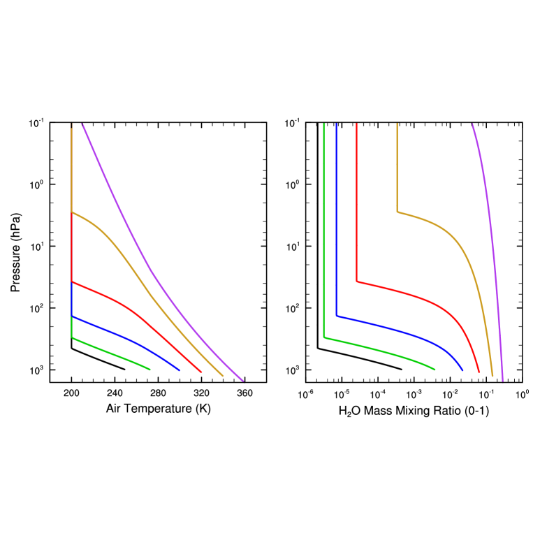
Figure 1: Input (a) air temperature and (b) water vapor mass mixing ratio used in the radiative-transfer calculations. Surface temperatures are 250, 273, 300, 320, 340, and 360 K.

Our calculations are performed in a similar manner to Kasting (1988) and Kasting et al. (1993), but cover a smaller range of temperatures, as shown in Fig. 1. Specifically, we perform all shortwave calculations with a top-of-atmosphere fixed stellar flux (340 W m^-2) and longwave calculations with a variety of fixed surface temperatures and assumed atmospheric temperature profiles. Note that the outgoing longwave radiation (infrared emission to space) from our longwave calculations does not necessarily balance the absorbed shortwave. In order to interpret our results, we will make use of the “effective solar flux” concept Kasting (1988) in section 5 to estimate the solar flux that would allow equilibrium, which we will explain at that point.

We set the surface temperature to 250, 273, 300, 320, 340, and 360 K. We were not able to get the AM2 scheme to converge for temperatures of 320 K and above, so we will only address the results of AM2 experiments at 250, 273, and 300 K. The temperature structures are moist adiabatic profiles overlain by a 200-K isothermal stratosphere. The atmosphere is assumed to be saturated in water vapor (relative humidity is equal to one). The volume mixing ratio of water vapor in the stratosphere is set equal to its value at the tropopause. The atmosphere is assumed to be Earth-like, namely 1-bar N₂, variable H₂O, and 376 ppmv CO₂. We do not include other gases, clouds, or aerosols. Because the total pressure of the atmosphere is variable as temperature changes and because we fix the volume mixing ratio of CO₂, the absolute mass of CO₂ is not constant, but this should not affect our results significantly for CO₂ at such low concentrations. For example, as the surface temperature increases from 300 to 360 K, the surface pressure increases from 1019 to 1598 hPa due to the increase water vapor, and the vertically integrated mass of 376-ppmv CO₂ increases from 5.7 to 8.9 kg m^-2. If assume the radiative forcing at the tropopause for doubling CO₂ concentration is about 4 W m^-2 (Collins et al., 2006), the increased radiative forcing due to the increase of CO₂ mass is about 2.1 W m^-2. This forcing should be uniform across models (so it will not cause discrepancies) and it is one order of magnitude smaller than the differences of tens of W m^-2 in radiative fluxes at high temperatures among the models found in our calculations below.

The incoming stellar flux at the top of the models is 340 W m^-2 in all calculations. By default, the surface has a uniform albedo of 0.25 in the shortwave. An exception is the surface albedo in SMART, which was set to 0.25 for wavelengths shorter than 3 $\mu$m and to zero at longer wavelengths, due to a mistake on our part. This means SMART absorbs more shortwave radiation at the surface and underestimates the reflected, upward shortwave flux. The magnitude of this underestimation, however, should be less than $\approx$ 1.6 W m^-2, due to the fact that only a small fraction of the stellar energy is in the region of wavelengths longer than 3 $\mu$m for both G and M stars. For longwave calculations, the surface is assumed to have a uniform emissivity equal to one. All models have a top pressure of 0.1 hPa. The number of vertical levels is 75 in SMART, 150 for longwave and 75 for shortwave in LBLRTM, and 301 in the band models. Due to the high spectral resolution and the long-time integrations, we had to limit the number of vertical levels in the two line-by-line models (SMART and LBLRTM) so that the calculations would be numerically feasible. The vertical resolution has a very small effect on radiative fluxes, less than $\approx$ 0.01 W m^-2 (Collins et al., 2006). The solar zenith angle is 60^∘ in all the calculations.

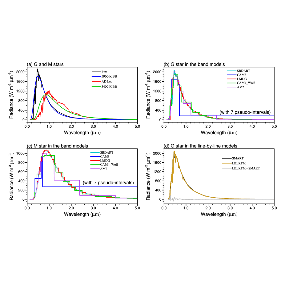
Figure 2: (a) Realistic stellar spectra and the corresponding blackbody spectra. (b) Representation of the G-star spectrum in the band models. (c) Same as (b), but for an M star. There are 7 pseudo-intervals at the near-infrared region in CAM3; in AM2, there are 38 pseudo-intervals for all bands, which are not shown in the figure. (d) Representation of the G-star spectrum in two line-by-line models and the difference between them. For comparison, both SMART and LBLRTM in (d) have been converted to have a spectral resolution of approximately 0.0025 $\mu$m. In all panels, differences at wavelengths longer than 5 $\mu$m are very small and thus are not shown.

We explore two stellar spectra, the real solar spectrum and an idealized, 3400-K blackbody spectrum (representing an M dwarf), except where explicitly noted otherwise. These two spectra, as well as other two spectra (a 5900-K blackbody and the real spectrum of the M dwarf AD Leo), and their representations in the models are shown in Fig. 2. The wavelength corresponding to the maximum spectral radiance in units of W m^-2 $\mu$m^-1 is $\approx$ 0.5 $\mu$m for the G star and $\approx$ 0.8 $\mu$m for the M star. The two line-by-line models have hundreds of thousands of spectral intervals. SBDART is a high-resolution band model and has 369 intervals in the stellar spectrum. In the broadband models, the stellar spectrum is divided into 19, 18, 23, and 36 spectral and pseudo-spectral intervals in CAM3, AM2, CAM4_Wolf, and LMDG, respectively. For instance, CAM3 has seven spectral intervals for O₃, one for the visible, three for CO₂, and seven near-infrared, pseudo-spectral intervals for H₂O. These pseudo-spectral intervals are employed to keep the number of spectral intervals as small as possible while fitting radiative heating rates to be close to the results of line-by-line calculations (Briegleb, 1992). The spectral intervals are finer in the visible region than in the near-infrared region in all band models. This is because these models were developed to simulate the climates of planets with Earth-like atmospheres and with Sun-like host stars. LMDG uses 16 gauss points for calculations of the cumulated distribution function of absorption data for each spectral interval, and CAM4_Wolf uses 8 gauss points per interval except at the intervals between 500 and 820 cm^-1, where 16 gauss points are used.

The output quantities from each model include (1) shortwave and longwave fluxes at the surface and at the top of the atmosphere, (2) upward and downward shortwave and longwave fluxes at each level of the atmosphere, (3) (optionally) spectra at the surface and/or at the top of the atmosphere. In this paper, for convenience and consistent with standard terminology, “longwave” refers to the thermal infrared emission from the planet, and “shortwave” refers to the stellar energy from the star. Although the shortwave and longwave overlap somewhat in the near-infrared, treating them separately still conserves energy, since the shortwave module does not consider the thermal energy and the longwave module does not consider the stellar energy.

3 Comparison of Longwave Radiation

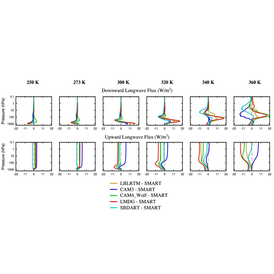
Figure 4: Differences in longwave flux between LBLRTM, CAM3, CAM4_Wolf, LMDG, SBDART, and SMART as a function of pressure and for surface temperatures from 250 to 360 K. Upper panels: differences in downward longwave flux; lower panels: differences in upward longwave flux. Note that longwave Fluxes from AM2 are unavailable.

Outgoing longwave radiation (OLR) fluxes at the top of the atmosphere (TOA) as a function of surface temperature are shown in Fig. 3(a). At low temperatures, all the models agree well with each other, while at high temperatures, the differences among the models become larger. The model spreads in the OLR are 5, 10, 17, and 25 W m^-2 at surface temperatures of 250, 300, 320, and 360 K, respectively. At the surface, the differences in net longwave flux are relatively small, less than 15 W m^-2 (Fig. 3(b)), since the atmosphere near the surface becomes optically thick, especially once the surface temperature is above 320 K. In the troposphere, the differences in downward longwave flux can be greater than those at the surface and at the TOA (Fig. 4).

In general, LMDG has the lowest OLR and the strongest greenhouse effect, whereas CAM3 has the highest OLR and the weakest greenhouse effect. In LMDG, SMART, and CAM4_Wolf, the OLR curves level out as the surface temperature is increased from 340 to 360 K. In CAM3, SBDART, and LBLRTM, however, the OLR curves keep increasing although at a small rate. For these three models, the maximum surface temperature of 360 K examined here may be not high enough to obtain their OLR limit, or they do not become optically thick at all wavelengths at high temperatures (Goldblatt et al., 2013). The existence and the value of the OLR limit are very important for the runaway greenhouse state. In LMDG, SMART, and CAM4_Wolf, the OLR limit is $\approx$ 287, 301, and 292 W m^-2, respectively.

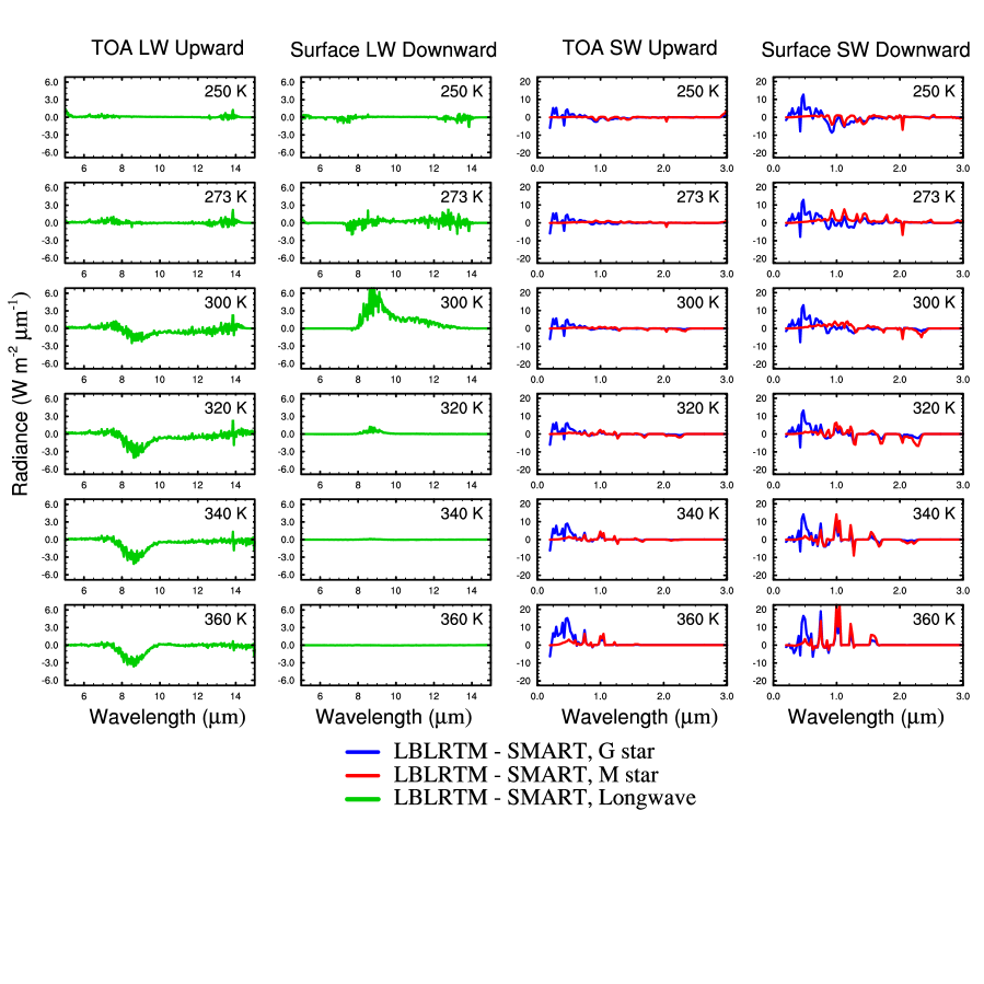
Figure 5: Shortwave (SW) and longwave (LW) spectral differences between the two line-by-line models, LBLRTM minus SMART. First column: upward longwave at the top of atmosphere; second column: downward longwave at the surface; third column: upward shortwave at the top of atmosphere; and fourth column: downward shortwave at the surface. For comparison, both models have been converted to have a spectral resolution of approximately 0.0025 $\mu$m. Differences at wavelengths between 3 and 5 $\mu$m and longer than 15 $\mu$m are relatively small and thus are not shown. In the third column, a part of the difference in wavelengths shorter than 1.0 $\mu$m is due to the difference in input solar spectra (see Fig. 2(d)).

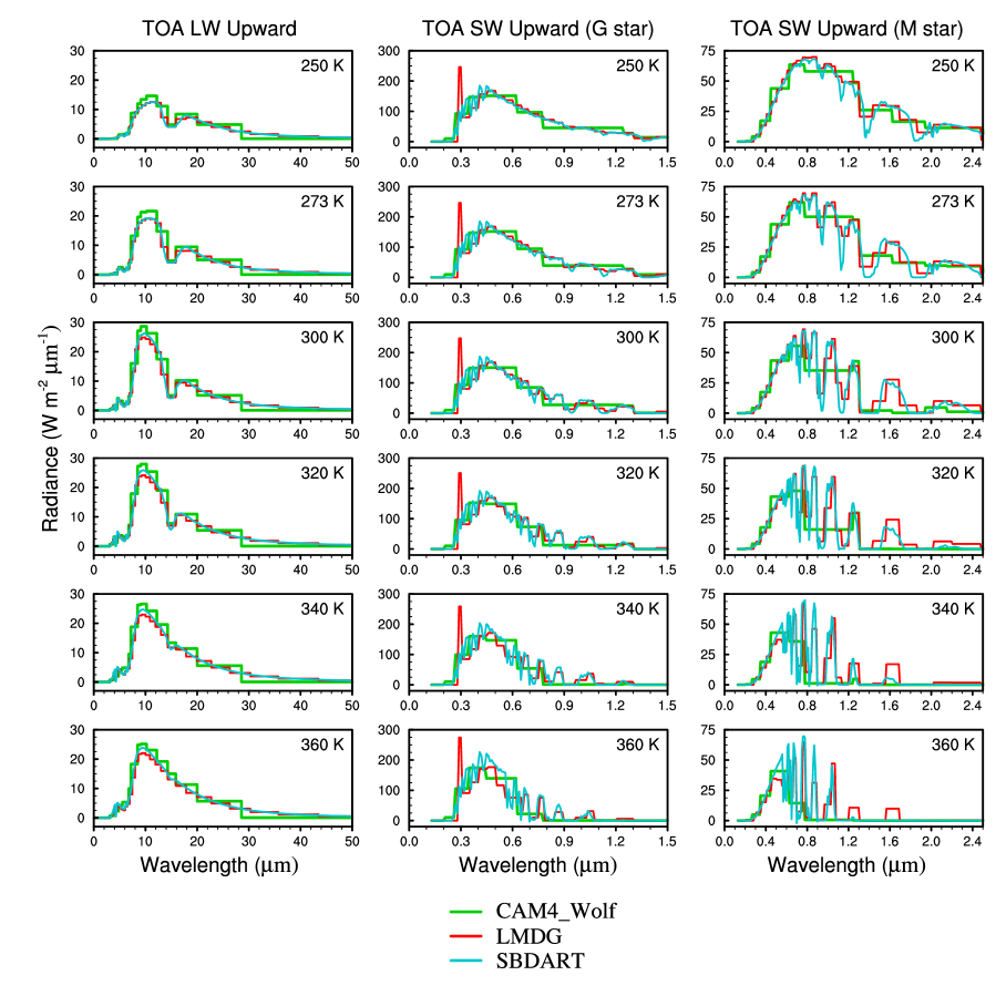
Figure 6: Longwave and shortwave spectra for the three correlated-$k$ models, CAM4_Wolf, LMDG, and SBDART. First column: upward longwave spectra at the top of atmosphere; second column: upward shortwave spectra at the top of atmosphere for G star; and third column: same as the second column, but for M star. In LMDG, a sharp bump exists at around 0.28 $\mu$m for G star (second column); this is because LMDG assigns all energy at wavelengths shorter than 0.28 $\mu$m to the narrow band between 0.28–0.30 $\mu$m. Spectra from CAM3 and AM2 are unavailable.

Between the two line-by-line models, SMART and LBLRTM, the difference in the OLR is mainly from the H₂O window region around 10 $\mu$m, where SMART absorbs less energy than LBLRTM (Fig. 5). This is likely due to different assumptions in water vapor continuum absorption (Table 1). Among the three models using the correlated-$k$ method, LMDG, CAM4_Wolf, and SBDART, the difference in the OLR is also mainly from the window region of around 10 $\mu$m (left panels of Fig. 6), which again emphasizes that differences in water vapor continuum absorption assumptions likely drive the inter-model spread in longwave behavior. Additionally, LMDG and SBDART appear to emit more than CAM4_Wolf at wavelengths longer than 28 $\mu$m.

4 Comparison of Shortwave Radiation

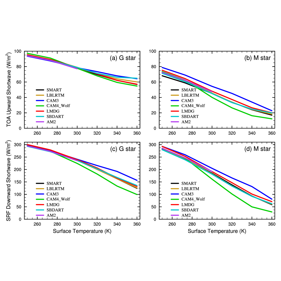
Figure 7: Shortwave fluxes for a G star (left panels) and for an M star (right panels) as a function of surface temperature from 250 to 360 K for all models: SBDART, LMDG, AM2, CAM3, CAM4_Wolf, SMART, and LBLRTM. (a) and (b): upward shortwave flux at the top of atmosphere; (c) and (d): downward shortwave flux at the surface.

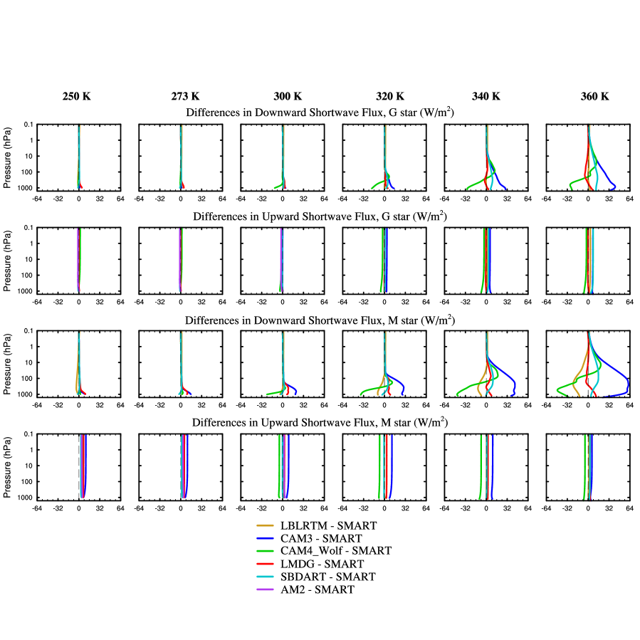
Figure 8: Differences in shortwave flux between LBLRTM, CAM3, CAM4_Wolf, LMDG, SBDART, AM2, and SMART as a function of pressure and for surface temperatures from 250 to 360 K. First row: Downward shortwave flux for a G star; second row: upward shortwave flux for a G star; third row: downward shortwave flux for an M star; and fourth row: Upward shortwave flux for an M star.

Fig. 7 shows upward shortwave radiation flux at the TOA and downward shortwave radiation flux at the surface as a function of surface temperature. All the models show that the upward and downward shortwave fluxes decrease with increasing surface temperature. This is mainly due to the increase in shortwave absorption by water vapor. Under the solar spectrum, the difference increases with temperature and the maximum difference of the shortwave flux among the models is less than $\approx$ 10 W m^-2 at the TOA, but can reach 60 W m^-2 at the surface. The increase in spread of the surface flux among models at higher temperatures is mostly due to the divergence in behavior of only two models, CAM3 and CAM4_Wolf. In general, the differences in downward shortwave flux near the surface and in the troposphere are much larger than those at the TOA (Fig. 8). Moreover, the differences in upward shortwave flux among the models are much smaller than those in downward shortwave flux. This is due to the fact that the surface absorbs 75% of the downward energy.

Under the M-star spectrum, the upward shortwave flux at the TOA and the downward shortwave flux at the surface are much less than those under the solar spectrum (right panels of Fig. 7). This is due to the redder M-star spectrum, which leads to more absorption by water vapor and less Rayleigh scattering (Pierrehumbert, 2010). The maximum difference among the models, however, is larger than that under the solar spectrum: 20 W m^-2 at the TOA and 90 W m^-2 at the surface. For both G- and M-star spectra, CAM3 has the smallest shortwave absorption and the largest Rayleigh scattering, while CAM4_Wolf has the largest shortwave absorption and the smallest Rayleigh scattering, especially once the surface temperature is equal to or higher than 300 K. When the surface temperature is less than 300 K, the difference among all the models is less than 15 W m^-2.

These models use different absorption line databases, different spectral resolutions, different methods for H₂O continuum absorption, and different multiple scattering schemes (see Table 1), all of which affect the shortwave radiation. For instance, as shown in the Supplementary Information of Goldblatt et al. (2013), the new HITRAN line database (e.g., HITRAN2008) has stronger shortwave absorption than the old HITRAN line database (e.g., HITRAN2000). Moreover, CAM3, AM2, and CAM4_Wolf have very coarse spectral resolutions, while LBLRTM, SMART, SBDART and LMDG have relatively fine resolutions. This could also cause differences among the models. Preliminary tests using CAM4_Wolf show that increasing the number of spectral intervals causes a significant improvement on the shortwave flux calculations (Kopparapu, Haqq-Misra, & Wolf, in preparation). The high resolution codes—LBLRTM, SMART, and SBDART are able to resolve individual absorption bands of water vapor in the near-infrared region (Figs. 5 and 6). LMDG, which has 36 shortwave spectral intervals, is also able to somewhat resolve the individual absorption and window bands separately (Fig. 6). On the contrary, CAM4_WOLF, CAM3, and AM2 must combine numerous near-infrared bands and window regions into larger spectral intervals. This can lead to errors, such as the fact that near-infrared absorption by CO₂ at 4.3 $\mu$m is not considered in CAM3 (Collins et al., 2006). There may also be some unknown parameters and errors in individual models, which could cause differences among the models.

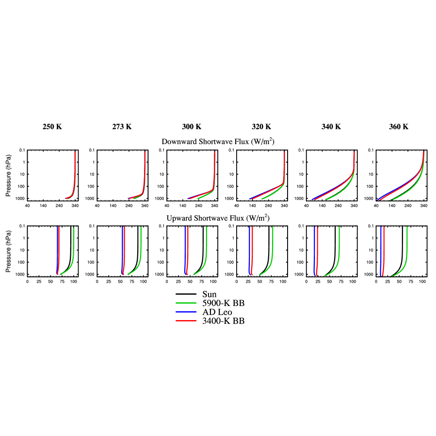
Figure 9: Shortwave fluxes for four different stellar spectra: the Sun, a 5900-K blackbody, AD Leo, and a 3400-K blackbody, calculated using the line-by-line model SMART. Upper panels: downward shortwave flux; lower panels: upward shortwave flux.

The influence of stellar spectrum on the radiative fluxes is further shown in Fig. 9. Using the line-by-line model SMART, we calculate downward and upward shortwave radiative fluxes under four different stellar spectra: the Sun, a 5900-K blackbody, the AD Leo, and a 3400-K blackbody. Primarily due to the wavelength dependence of shortwave absorption by water vapor, the differences in the radiation fluxes are significant between G- and M-star spectra, as has been previously found by others (e.g., Kasting et al., 1993; Pierrehumbert, 2010; Kopparapu et al., 2013; Shields et al., 2013, 2014; Godolt et al., 2015). Rayleigh scattering is also wavelength-dependent, but its effect is much smaller than that of water vapor absorption (Halthore et al., 2005). Moreover, the differences between a realistic stellar spectrum and its corresponding blackbody spectrum are relatively small, for both G and M stars. For instance, the maximum difference in the upward shortwave flux at the TOA between the AD Leo and the 3400-K blackbody is only $\approx$ 7 W m^-2.

5 Discussion: The Inner Edge of the Habitable Zone

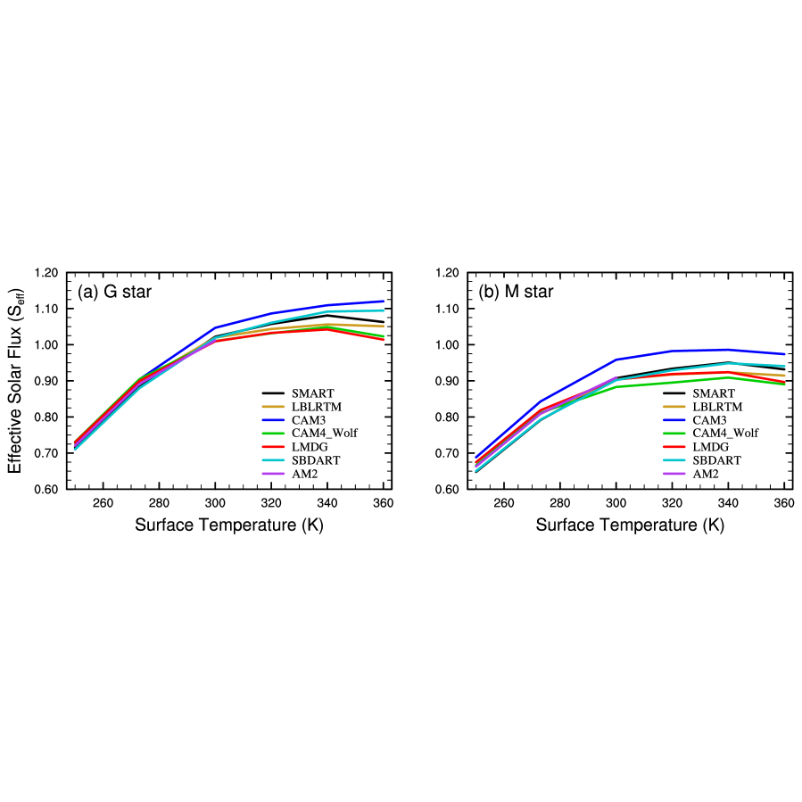
Figure 10: Effective solar flux for all models for (a) a G star and (b) an M star. The effective solar flux is defined as the ratio of outgoing longwave radiation to absorbed shortwave radiation. It is the factor by which present Earth’s solar flux would need to be multiplied in order to maintain a given surface temperature.

Now that we have explored the differences in radiative transfer among the models, it is important to put these differences in context in terms of the effect they can have on the inner edge of the habitable zone. One way we can approximate the inner edge based on our fixed atmospheric temperature profile simulations is by using the effective solar flux (S${}_{\textrm{eff}}$, Kasting, 1988), which is defined as the ratio of the outgoing longwave radiation to the total shortwave radiation absorbed by the planet (net shortwave at the TOA). S${}_{\textrm{eff}}$ corresponds to the factor by which one would have to multiply Earth’s solar flux in order to maintain a given surface temperature, and we have plotted it in Fig. 10. The maximum difference in S${}_{\textrm{eff}}$ is $\approx$ 3 % between the two line-by-line models and $\approx$ 10 % among the band models, which corresponds to $\approx$ 10 and $\approx$ 34 W m^-2 in the global mean, respectively. This shows that uncertainty in radiative transfer, even neglecting more complicated processes such as clouds and areas of sub-saturation, has a fairly significant effect on estimates of the inner edge of the habitable zone.

We should also note that similarity in S${}_{\textrm{eff}}$ can mask differences in model behavior. For example CAM4_WOLF and LMDG produce very similar values of S${}_{\textrm{eff}}$ (Fig. 10), but this results from the fact that, at a given surface temperature, CAM4_WOLF both emits more outgoing longwave radiation (Fig. 3) and absorbs more shortwave (Fig. 7) than LMDG. Moreover, even though the 1D calculations indicate that CAM4_WOLF and LMDG produce a runaway greenhouse at a stellar flux within about 1 % of each other for a G-star spectrum, 3D calculations show that a runaway greenhouse occurs for Earth when the solar constant is increased by 10 % in LMDG (Leconte et al., 2013), and has not yet occurred when the solar constant is increased by 21 % in CAM4_WOLF (Wolf & Toon, 2015). This difference could be caused simply by differences in simulations of sub-saturated regions and clouds, or it could result from more complicated feedbacks between atmospheric dynamics and the detailed differences in longwave and shortwave behavior between the two models mentioned above. This motivates a full comparison of 3D global climate models, which we are currently pursuing.

It would be encouraging if we could find some sort of relation between the age of the line database and water vapor continuum assumptions made by the models (Table 1) and similarity in model behavior. In the longwave, this is certainly not the case. For example, the models with the oldest databases (SBDART with HITRAN1996) and the newest databases (SMART with HITEMP2010 and HITRAN2012) yield almost identical outgoing longwave radiation (Fig. 3). In the shortwave, it does appear that models using databases developed within the past ten years clump together (Fig. 7), which may indicate that our understanding of shortwave absorption by large amounts of water vapor is converging, although it is always possible that the next generation databases will overturn this trend. In any case, our work emphasizes the need to develop more accurate line and continuum databases, and to try to constrain them with actual data (rather than just theoretical calculations) insofar as this is possible.

6 Conclusion

We have compared seven radiative transfer models that are currently being used to estimate the inner edge of the habitable zone. We found that there are significant differences among the models in both shortwave and longwave radiative fluxes, especially in the troposphere and at the surface. The maximum difference in radiative fluxes is on the order of tens of watts per square meter, and the uncertainty in estimating the insolation threshold of the inner edge of the habitable zone is about 10 % of the present Earth’s solar constant among the band models and about 3 % between the two line-by-line models. Our results suggest two ways to improve the radiative transfer in climate simulations of exoplanets. One is to improve the absorption coefficients and continuum behavior of water vapor, especially in the infrared window region and in the entire visible region, and the other one is to increase the resolution of stellar spectra in broadband models.

Table 1: Main characteristics of 1D radiative transfer models^a employed in our intercomparison, including spectral line databases for H₂O absorption (HITRAN), the number of vertical levels (Lev.), the number of intervals for stellar spectra (Int.), and methods for calculating absorption coefficients, H₂O continuum absorption (H₂O Cont.), and multiple scattering.

Modelsb	HITRAN	Lev.	Int.	Absor. Coeff.	H2O Cont.	Multiple Scattering	Examiners
SBDART	1996	301	369	correlated-$k$	CKD2.3	Stamnes et al. (1988)	Wang
CAM3c	2000	301	19	absorp./emis.	CKD2.4	Briegleb (1992)	Yang
AM2	2000	301	18	exponential sum	CKD2.1	Edwards & Slingo (1996)	Feldl
CAM4_Wolf	2004	301	23	correlated-$k$	MT_CKD2.5	Toon et al. (1989)	Wolf
LMDG	2008	301	36	correlated-$k$	CKD2.4	Toon et al. (1989)	Leconte
LBLRTM	2008	150d	$>$$10^{4}$	line-by-line	MT_CKD2.5	Moncet & Clough (1997)	Wolf
SMART	2010e	75	$>$$10^{4}$	line-by-line	$\chi$-factors	Stamnes et al. (1988)	Goldblatt

a. SBDART is a software tool for computing radiative transfer, developed by Ricchiazzi et al. (1988). CAM version 3 (CAM3) is a 3D atmospheric general circulation model (GCM), developed at NCAR. CAM4_Wolf is CAM version 4 (CAM4) but with a new radiative transfer module, developed by E. T. Wolf. AM2 is a 3D GCM developed at NOAA/GFDL. LMDG is the 3D Laboratoire de Météorologie Dynamique (LMD) Generic Model, developed at LMD, Paris, France. Here, CAM3, AM2, CAM4_Wolf, and LMDG are the pure radiative transfer modules of the corresponding 3D GCMs. SMART is a line-by-line radiative transfer models, developed by David Crisp at NASA’s JPL in California. LBLRTM is another line-by-line model developed at the Atmospheric and Environmental Research, Inc. (AER).
b. Appropriate references for SBDART: Ricchiazzi et al. (1988) and Yang et al. (2000); for CAM3: Collins et al. (2002) and Ramanathan & Downey (1986); for AM2: Edwards & Slingo (1996) and Freidenreich & Ramaswamy (1999); for CAM4_Wolf: Wolf & Toon (2015); for LMDG: Wordsworth et al. (2010a, b); for LBLRTM: Clough et al. (2005, 1992); and for SMART: Meadows & Crisp (1996) and Crisp (1997). CAM3 uses an absorptivity/emissivity formulation for absorption coefficients. Appropriate references for H₂O continuum absorption are Clough et al. (1989, 2005) and Mlawer et al. (2012). All the line databases are developed at the Atomic and Molecular Physics Division, Harvard-Smithsonian Center for Astrophysics under the direction of L. S. Rothman (see Rothman et al., 2013, and references therein).
c. Pure radiative transfer calculations with CAM3 were done with CliMT (http://climdyn.misu.su.se/climt/). CliMT is an object-oriented climate modeling and diagnostics toolkit, developed by Rodrigo Caballero.
d. 150 levels for longwave calculations, and 75 levels for shortwave calculations.
e. HITEMP2010 for H₂O and HITRAN2012 for CO₂.

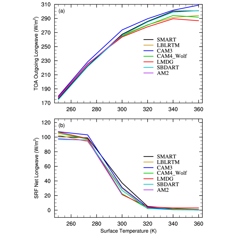
Figure 3: (a) Outgoing longwave radiation at the top of the atmosphere (TOA), and (b) net longwave radiation at the surface (SRF) as a function of surface temperature for all of the models from 250 to 360 K.

References

- Abe (1993) Abe, Y., Lithos, 30, 223
- Abe et al. (2011) Abe, Y., Abe-Ouchi, A., Sleep, N. H., & Zahnle, K. J., 2011, Astrobiology, 11(5), 443
- Boucher et al. (2001) Boucher, O., et al. 2001, in Climate Change 2001: The Scientific Basis, Houghton, J. T., et al. (eds.), Cambridge University Press, USA
- Briegleb (1992) Briegleb, B. P. 1992, J. Geophys. Res., 97, 7603
- Clough et al. (1992) Clough, S. A., Iacono, M. J., & Moncet, J.-L. 1992, J. Geophys. Res., 97, 15761
- Clough et al. (1989) Clough, S. A., Kneizys, F., & Davies, R. R. 1989, Atmos. Res., 23, 229
- Clough et al. (2005) Clough, S. A., Shephard, M. W., Mlawer, E. J., Delamere, J. S., Iacono, M. J., Cady-Pereira, K., Boukabara, S., & Brown, P. D. 2005, J. Quant. Spectrosc. Ra. Trans., 91, 233
- Collins et al. (2002) Collins, W. D., Hackney, D. P., & Edwards, D. P. 2002, J. Geophys. Res., 107(D22), doi: 10.1029/2001JD001365
- Collins et al. (2006) Collins, W. D., Ramaswamy, V., Schwarzkopf, M. D., et al. 2006, J. Geophys. Res., 111, doi:10.1029/2005JD006713
- Crisp (1997) Crisp, D. 1997, Geosphy. Res. Lett., 24, 571
- Edwards & Slingo (1996) Edwards, J. M., & Slingo, A. 1996, Quart. J. Roy. Meteor. Soc., 122, 689
- Freidenreich & Ramaswamy (1999) Freidenreich, S. M., & Ramaswamy, V. 1999, J. Geophys. Res., 104, 31389
- Forget et al. (1999) Forget, F., Hourdin, F., Fournier, R., et al. 1999, J. Geophys. Res., 104, 24155
- Fouquart et al. (1991) Fouquart, Y., Bonnel, D., & Ramaswamy, V. 1991, J. Geophys. Res., 96, 8955
- Godolt et al. (2015) Godolt, M., Grenfell, J. L., Hamann-Reinus, A., Kitzmann, D., Kunze, M., Langematz, U., von Paris, P., Patzer, A. B. C., Rauer, H., & Stracke, B. 2015, Planetary and Space Science, 111, 62
- Goldblatt & Watson (2012) Goldblatt, C., & Watson, A. J. 2012, Phil. Trans. R. Soc. A., 370, 4197
- Goldblatt et al. (2013) Goldblatt, C., Robinson, T. D., Zahnle, K. J., & Crisp, D. 2013, Nature Geosci., 6, 661
- Halthore et al. (2005) Halthore, R. N., Crisp, D., Schwartz, S. E., et al. 2005, J. Geophys. Res., 110, D11206, doi:10.1029/2004JD005293
- Iacono et al. (2008) Iacono, M. J., Delamere, J. S., Mlawer, E. J., Shephard, M. W., Clough, S. A., & Collins, W. D. 2008, J. Geophys. Res., 113, D13103, doi:10.1029/2008JD009944
- Kasting (1988) Kasting, J. F. 1988, Icarus, 74, 472
- Kasting (2010) Kasting, J. F. 2010, How to find a habitable planet, Princeton University Press, New Jersey, USA
- Kasting et al. (2014) Kasting, J. F., Kopparapu, R., Ramirez, R. M., & Harman C. E. 2014, PNAS, 111(35), 12641
- Kasting et al. (1993) Kasting, J. F., Whitmire, D. P., & Reynolds, R. T. 1993, Icarus, 101, 108
- Kodama et al. (2015) Kodama, T., Genda, H., Abe, Y., Zahnle, K. J. 2015, ApJ, 812, 2
- Kopparapu et al. (2013) Kopparapu, R. K., Ramirez, R., Kasting, J. F., et al. 2013, ApJ, 767, 131
- Kopparapu et al. (2014) Kopparapu, R. K., Ramirez, R., Kasting, J. F., et al. 2014, ApJ Lett., 787, L29
- Leconte et al. (2013) Leconte, J., Forget, F., Charnay, B., Wordsworth, R., & Pottier, A. 2013, Nature, 504, 268
- Masson-Delmotte et al. (2013) Masson-Delmotte, V., Schulz, M., Abe-Ouchi, A., et al. 2013, in Climate Change 2013: The Physical Science Basis, Stocker, T. F., et al. (eds.), Cambridge University Press, USA
- Meadows & Crisp (1996) Meadows, V. S., & Crisp, D. 1996, J. Geophys. Res. 101, 4595
- Mlawer et al. (2012) Mlawer, E. J., Payne, V. H., Moncet, J.-L., Delamere, E. S., Alvarado, M. J., & Tobin, D. C. 2012, Phil. Trans. R. Soc. A, 370, 2520
- Moncet & Clough (1997) Moncet, J.-L., & Clough, S. A. 1997, J. Geophys. Res., 102, 21853, doi:10.1029/97JD01551
- Nakajima et al. (1992) Nakajima, S., Hayashi, Y.-Y., & Abe, Y. 1992, J. Atmos. Sci., 49, 2256
- Pierrehumbert (2010) Pierrehumbert, R. T. 2010, Principles of Planetary Climate, Cambridge University Press, USA
- Ramanathan & Downey (1986) Ramanathan, V., & Downey, P. A. 1986, J. Geophys. Res., 91, 8649
- Rothman et al. (2013) Rothman, L. S., Gordon, I. E., Babikov, Y., et al. 2013, J. Quant. Spectrosc. Ra. Trans., 130, 4
- Ricchiazzi et al. (1988) Ricchiazzi, P., Yang, S., Gautier, C., & Sowle, D. 1988, BAMS, 79(10), 2101
- Shields et al. (2014) Shields, A. L., Bitz, C. M., Meadows, V. S., Joshi, M. M., & Robinson, T. D. 2014, ApJ Lett., 785, L9
- Shields et al. (2013) Shields, A. L., Meadows, V. S., Bitz, C. M., Pierrehumbert, R. T., Joshi, M. M., & Robinson, T. D. 2013, Astrobiology, 13(8), 715
- Stamnes et al. (1988) Stamnes, K., Tsay, S. C., Wiscombe, W., & Jayaweera, K. 1988, Appl. Opt., 27, 2502
- Toon et al. (1989) Toon, O. B., McKay, C. P., Ackerman, T. P., & Santhanam, K. 1989, J. Geophys. Res., 94, 16287
- Walker et al. (1981) Walker, J. C. G., Hays, P. B., & Kasting, J. F. 1981, J. Geophys. Res., 86, 9776
- Wolf & Toon (2014) Wolf, E. T., & Toon, O. B. 2014, Geophys. Res. Lett., 41, 167
- Wolf & Toon (2015) Wolf, E. T., & Toon, O. B. 2015, J. Geophys. Res.: Atmospheres, 120, 5775
- Wordsworth et al. (2010a) Wordsworth, R., Forget, F., & Eymet, V. 2010a, Icarus, 210, 992
- Wordsworth et al. (2010b) Wordsworth, R., Forget, F., Selsis, F., Madeleine, J.-B., Millour, E., & Eymet, V. 2010b, A&A, 522, A22
- Yang et al. (2000) Yang, S., Ricchiazzi, P., & Gautier, C., 2000, J. Quant. Spectrosc. Ra. Trans, 64, 585
- Yang et al. (2013) Yang, J., Cowan, N. B., and Abbot, D. S. 2013, ApJ Lett., 771, L45
- Yang et al. (2014) Yang, J., Boué, G., Fabrycky, D. C., and Abbot, D. S. 2014, ApJ Lett., 787, L2