Studying flavor-changing neutral $tqZ$ couplings : Current constraints and future prospects

Zenrō HIOKI${}^{\>1),\>}$ Kazumasa OHKUMA${}^{\>2),\>}$ and Akira UEJIMA${}^{\>2),\>}$

$1)$ Institute of Theoretical Physics, University of Tokushima

Tokushima 770-8502, Japan

$2)$ Department of Information and Computer Engineering,

Okayama University of Science

Okayama 700-0005, Japan

ABSTRACT

Possible non-standard $tuZ$ and $tcZ$ interactions, which induce flavor-changing neutral-current decays of the top quark, are studied in the effective-Lagrangian framework. The corresponding Lagrangian consists of four kinds of non-standard couplings coming from $SU(3)\times SU(2)\times U(1)$ invariant dimension-6 effective operators. The four coupling constants in each interaction are treated as complex numbers independent of each other, and constraints on them are derived by using the present experimental limits of the branching fractions for $t\to uZ$ and $t\to cZ$ processes. Future improvements of those constraints are also discussed as well as possibilities of measurements of these couplings at the High-Luminosity Large Hadron Collider.

PACS:    12.38.Qk,    12.60.-i,    14.65.Ha

1. Introduction

The Large Hadron Collider (LHC) established the standard model of particle physics by discovering the Higgs boson [1, 2], which was the last piece in the model. Meanwhile, the LHC has also been searching for new particles which are not included in the framework of the standard model, however, any signal indicating their existence has not been directly observed yet even at 13 TeV. Therefore, precise measurements of various standard-particle processes have received a lot of attention as an indirect search for new physics. In particular, processes caused by a Flavor-Changing Neutral Current (FCNC) are quite attractive as a target for current and future measurements. That is, the FCNC is strongly suppressed by the Glashow-Iliopoulos-Maiani mechanism in the standard model [4], and hence observation of such processes will be good indication of new-physics effects.

On the other hand, the top quark, which is the heaviest in the observed elementary-particle spectrum, is also expected to play a crucial role in new-physics search (see, e.g., [3] and its references) because of the following reasons:
(1) The top quark decays without receiving non-perturbative hadronization effects due to a very short lifetime originated from its huge mass close to the electroweak scale [5, 6]. This unique quality is suitable for future clean analyses of its interactions, which have not been studied enough accurately yet in comparison with the other lighter quarks and still might have room to hide some non-standard terms.
(2) The $C\!P$-violation in the top-quark sector is known to be very small within the standard model. Therefore, if any sizable $C\!P$-violation effects are measured in top-quark productions and/or decays, they can be interpreted to come from a possible new physics beyond the standard model.
(3) The top quark strongly interacts with the yet-mysterious Higgs boson. Thus, detailed studies of top-quark interactions would be useful to explore the mechanism of electroweak symmetry breaking as well as properties of the Higgs boson.

Considering them altogether and also taking into account the fact that top-quark precise measurement is one of the most important missions at future facilities (e.g., High-Luminosity Large Hadron Collider, International Linear Collider, and Future Circular Collider), we focus in this letter on flavor-changing neutral-current decays of the top quark $t\to uZ$ and $t\to cZ$, and study to what extent we can draw valuable information on non-standard interactions that could induce these processes from the present experimental data. Their branching fractions are estimated to be of ${\cal O}(10^{-17})$ and ${\cal O}(10^{-14})$ respectively in the standard model[7], that is why observation of those processes will be a clear evidence of possible new physics beyond the standard model.

It is not that easy, however, to identify what kinds of new interactions had contributed to the processes, even if we observed some meaningful signals. In such a situation, the effective-Lagrangian approach which examines model-independently all the possible extensions of the standard-model interactions is one of the most promising methods for evaluating possible new-physics contributions.

Indeed, a lot of efforts have already been made to analyze the $tqZ$ interactions, where $q=u/c$, based on the effective Lagrangian in order to probe top-quark FCNC [7, 8, 9, 10, 11, 12, 13, 14, 15, 16, 17, 19, 20, 18, 21, 22]. In most of the studies, however, only some couplings included in the effective Lagrangian have been treated as free parameters at once fixing the others. Furthermore, these non-standard couplings tend to be restricted to real or partially imaginary numbers there, though they could be complex in general.

Although such limited analyses could be reasonable if the authors are implicitly considering some specific models, we here deal with all the non-standard couplings as complex numbers and regard those couplings as free independent parameters in order to perform a fully model-independent analysis. Thus, our results given below do not depend on any specific models. It never means, of course, that our results offer no helpful information for model-dependent new-physics studies. That is, they do not have to take into account the parameter space which has been excluded in our analyses.

The outline of this letter is as follows: After describing our calculational framework in section 2, we perform numerical analyses and show main results in section 3. There, we also present some related discussions. Finally, a summary is given in section 4.

2. Framework

The effective Lagrangian used here is constructed assuming that there exists some new physics characterized by an energy scale ${\mit\Lambda}$, and all the non-standard particles are much heavier than the colliding energies of the LHC. In this framework, new-physics phenomena are described by $SU(3)\times SU(2)\times U(1)$ invariant operators whose mass-dimension is six, and there are five kinds of operators that could contribute to the $tqZ$ interactions [23, 24, 25, 26]. The appropriate operators are extracted from Ref. [25] as follows:

$${\cal O}^{3,i3}_{\phi q} =i\left(\phi^{\dagger}\tau^{I}D_{\mu}\phi)(\bar{q}_{Li}\gamma^{\mu}\tau^{I}q_{L3}\right), \quad{\cal O}^{1,i3}_{\phi q} =i\left(\phi^{\dagger}D_{\mu}\phi)(\bar{q}_{Li}\gamma^{\mu}q_{L3}\right),$$

$${\cal O}^{i3}_{\phi u} =i\left(\phi^{\dagger}D_{\mu}\phi)(\bar{u}_{Ri}\gamma^{\mu}u_{R3}\right),$$

$${\cal O}^{i3}_{uW} =\left(\bar{q}_{Li}\sigma^{\mu\nu}\tau^{I}u_{R3}\right)\tilde{\phi}W^{I}_{\mu\nu}, \quad{\cal O}^{i3}_{uB\phi} =\left(\bar{q}_{Li}\sigma^{\mu\nu}u_{R3}\right)\tilde{\phi}B_{\mu\nu},$$

where subscripts $i$ and 3 stand for the quark generations, i.e., $i=1$ and $2$ correspond to the up and charm quarks, 3 corresponds to the top quark, respectively.

Using the above operators, we can write down the effective Lagrangian of $tqZ$ interactions describing phenomena around the electroweak scale as

$${\cal L}_{tqZ}=-\frac{g}{2\cos\theta_{W}}\Bigl{[}\,\bar{\psi}_{q}(x)\gamma^{\mu}(f_{1}^{L}P_{L}+f_{1}^{R}P_{R})\psi_{t}(x)Z_{\mu}(x)\Bigr{.}$$

$$\phantom{========}+\bar{\psi}_{q}(x)\frac{\sigma^{\mu\nu}}{M_{Z}}(f_{2}^{L}P_{L}+f_{2}^{R}P_{R})\psi_{t}(x)\partial_{\mu}Z_{\nu}(x)\,\Bigr{]},$$ (1)

where $g$ and $\theta_{W}$ are the $SU(2)$ coupling constant and the weak mixing angle, $P_{L/R}\equiv(1\mp\gamma_{5})/2$, and $f_{1/2}^{L/R}$ stand for the non-standard couplings defined as

$$f_{1}^{L} =\frac{v^{2}}{2{\mit\Lambda}^{2}}\left[C_{\phi q}^{(3,i3)}+C_{\phi q}^{(3,3i)*}-C_{\phi q}^{(1,i3)}-C_{\phi q}^{(1,3i)*}\right], \quad f_{1}^{R} =-\frac{v^{2}}{2{\mit\Lambda}^{2}}\left[C_{\phi u}^{i3}+C_{\phi u}^{3i*}\right],$$

$$f_{2}^{L} =-\frac{\sqrt{2}v^{2}}{{\mit\Lambda}^{2}}\left[C_{uW}^{3i*}\cos\theta_{W}-C_{uB\phi}^{3i*}\sin\theta_{W}\right],$$

$$f_{2}^{R} =-\frac{\sqrt{2}v^{2}}{{\mit\Lambda}^{2}}\left[C_{uW}^{i3}\cos\theta_{W}-C_{uB\phi}^{i3}\sin\theta_{W}\right].$$

As mentioned above, $f_{1/2}^{L/R}$ are treated as complex numbers independent of each other from the viewpoint of model-independent analysis.

3. Numerical analyses

We are now ready to derive allowed regions for the non-standard couplings. In the analyses, we use the following recent experimental data at 95 % confidence level:

• The total-decay width of the top quark, ${\mit\Gamma}^{t}$ [GeV] [27] ;

  $$4.8\times 10^{-2}\leq{\mit\Gamma}^{t}\leq 3.5$$ (2)

• The upper limits of the branching fractions for $t\to qZ$ decays [28];

  $$\begin{split}&{\rm Br}(t\to uZ)<1.7\times 10^{-4}\\ &{\rm Br}(t\to cZ)<2.3\times 10^{-4}\end{split}$$ (3)

Then, multiplying the minimum (maximum) value of ${\mit\Gamma}^{t}$ by ${\rm Br}(t\to uZ/cZ)$, the corresponding partial decay widths, ${\mit\Gamma_{tqZ}}$ [GeV], are obtained as

$$\begin{split}&0\leq{\mit\Gamma}_{tuZ}<8.1\times 10^{-6}~{}~{}(5.9\times 10^{-4}),\\ &0\leq{\mit\Gamma}_{tcZ}<1.1\times 10^{-5}~{}~{}(8.0\times 10^{-4}).\end{split}$$ (4)

In order to find constraints on $f_{1/2}^{L/R}$, we compare the experimental limits of ${\mit\Gamma_{tqZ}}$ in Eq.(4) with the one which is calculated from Eq.(2. Framework) as a function of $f_{1/2}^{L/R}$. More specifically, by varying the real and imaginary parts of each $f_{1/2}^{L/R}$ independently at the same time, we look for allowed regions of them numerically. In this analysis, we take as $m_{t}=172.5~{}{\rm GeV}$ and $M_{Z}=91.2~{}{\rm GeV}$ , and other physical constants are referred from the Review of Particle Physics  [29]. In addition, we do not neglect any order products of the non-standard couplings, though higher order products of those couplings tend to be out of consideration in many analyses. These computations are straightforward, but the parameter space to be explored is quite large, so the calculator with Graphics Processing Unit is used to perform them.

Table 3. Numerical analyses shows the obtained constraints on the $tuZ$-coupling parameters, where those over (under) the dashed lines in the rows marked by Min. and Max. are the minimum and maximum values of the allowed ranges derived from ${\mit\Gamma}_{tuZ}=8.1\times 10^{-6}~{}(5.9\times 10^{-4})$. Table 3. Numerical analyses is the same as Table 3. Numerical analyses but for the $tcZ$ couplings, where those over (under) the dashed lines are from ${\mit\Gamma}_{tcZ}=1.1\times 10^{-5}$ ($8.0\times 10^{-4}$).

Table 1: Current constraints on the $tuZ$-coupling parameters: Those over (under) the dashed lines in the rows denoted as Min. and Max. are the minimum and maximum of the allowed ranges coming from ${\mit\Gamma}_{tuZ}=8.1\times 10^{-6}~{}(5.9\times 10^{-4})$.

	$f_{1}^{L}$		$f_{1}^{R}$
	Re($f_{1}^{L}$)	Im($f_{1}^{L})$	Re($f_{1}^{R}$)	Im($f_{1}^{R}$)
Min.	$-5.5\times 10^{-3}$	$-5.5\times 10^{-3}$	$-5.5\times 10^{-3}$	$-5.5\times 10^{-3}$
2-5	$-4.7\times 10^{-2}$	$-4.7\times 10^{-2}$	$-4.7\times 10^{-2}$	$-4.7\times 10^{-2}$
Max.	$\phantom{-}5.5\times 10^{-3}$	$\phantom{-}5.5\times 10^{-3}$	$\phantom{-}5.5\times 10^{-3}$	$\phantom{-}5.5\times 10^{-3}$
2-5	$\phantom{-}4.7\times 10^{-2}$	$\phantom{-}4.7\times 10^{-2}$	$\phantom{-}4.7\times 10^{-2}$	$\phantom{-}4.7\times 10^{-2}$

	$f_{2}^{L}$		$f_{2}^{R}$
	Re($f_{2}^{L}$)	Im($f_{2}^{L})$	Re($f_{2}^{R}$)	Im($f_{2}^{R}$)
Min.	$-4.6\times 10^{-3}$	$-4.6\times 10^{-3}$	$-4.6\times 10^{-3}$	$-4.6\times 10^{-3}$
2-5	$-3.9\times 10^{-2}$	$-3.9\times 10^{-2}$	$-3.9\times 10^{-2}$	$-3.9\times 10^{-2}$
Max.	$\phantom{-}4.6\times 10^{-3}$	$\phantom{-}4.6\times 10^{-3}$	$\phantom{-}4.6\times 10^{-3}$	$\phantom{-}4.6\times 10^{-3}$
2-5	$\phantom{-}3.9\times 10^{-2}$	$\phantom{-}3.9\times 10^{-2}$	$\phantom{-}3.9\times 10^{-2}$	$\phantom{-}3.9\times 10^{-2}$

Table 2: Current constraints on the $tcZ$-coupling parameters: Those over (under) the dashed lines in the rows denoted as Min. and Max. are the minimum and maximum of the allowed ranges coming from ${\mit\Gamma}_{tcZ}=1.1\times 10^{-5}~{}(8.0\times 10^{-4})$.

	$f_{2}^{L}$		$f_{2}^{R}$
	Re($f_{2}^{L}$)	Im($f_{2}^{L})$	Re($f_{2}^{R}$)	Im($f_{2}^{R}$)
Min.	$-5.3\times 10^{-3}$	$-5.3\times 10^{-3}$	$-5.3\times 10^{-3}$	$-5.3\times 10^{-3}$
2-5	$-4.5\times 10^{-2}$	$-4.5\times 10^{-2}$	$-4.5\times 10^{-2}$	$-4.5\times 10^{-2}$
Max.	$\phantom{-}5.3\times 10^{-3}$	$\phantom{-}5.3\times 10^{-3}$	$\phantom{-}5.3\times 10^{-3}$	$\phantom{-}5.3\times 10^{-3}$
2-5	$\phantom{-}4.5\times 10^{-2}$	$\phantom{-}4.5\times 10^{-2}$	$\phantom{-}4.5\times 10^{-2}$	$\phantom{-}4.5\times 10^{-2}$

Comparing these two Tables, we find that the $tuZ$ couplings are more strongly restricted than the $tcZ$ couplings. Apparently it comes from the difference between the current experimental limits of each branching fraction. On the other hand, both the real and imaginary parts of $f_{1}^{L/R}$ and $f_{2}^{L/R}$ in each of the $tuZ$ and $tcZ$ couplings have the same minimum and maximum limits, respectively.

Table 3: Allowed minimum and maximum values of the $tuZ$ couplings for ${\mit\Gamma}_{tuZ}=8.1\times 10^{-6}$ in the case that Re($f_{1}^{L}$) is fixed to $5.5\times 10^{-3}$.

	$f_{1}^{L}$		$f_{1}^{R}$
	Re($f_{1}^{L}$)	Im($f_{1}^{L})$	Re($f_{1}^{R}$)	Im($f_{1}^{R}$)
Min.	$\,\;5.5\times 10^{-3}\;$	$-1.0\times 10^{-3}$	$-1.0\times 10^{-3}$	$-1.0\times 10^{-3}$
Max.	(Fixed)	$\phantom{-}1.0\times 10^{-3}$	$\phantom{-}1.0\times 10^{-3}$	$\phantom{-}1.0\times 10^{-3}$

	$f_{2}^{L}$		$f_{2}^{R}$
	Re($f_{2}^{L}$)	Im($f_{2}^{L})$	Re($f_{2}^{R}$)	Im($f_{2}^{R}$)
Min.	$-8.0\times 10^{-4}$	$-8.0\times 10^{-4}$	$-4.2\times 10^{-3}$	$-8.0\times 10^{-3}$
Max.	$\phantom{-}8.0\times 10^{-4}$	$\phantom{-}8.0\times 10^{-4}$	$-3.4\times 10^{-3}$	$\phantom{-}8.0\times 10^{-3}$

We here should comment about the results in the tables. What the allowed ranges express is: if we give one parameter a value outside its allowed range, we can no longer reproduce the width ${\mit\Gamma}_{tuZ}$ or ${\mit\Gamma}_{tcZ}$ which satisfies the inequalities in Eq.(4) however we vary the other parameters. Therefore they do not ensure that any combination of parameter values within the allowed areas is allowed by those inequalities. For example, when one of the parameters is assumed to take its maximum value listed in the tables (e.g., ${\rm Re}(f_{1}^{L})=5.5\times 10^{-3}$), we obtain more restrictive results for the remaining ones as shown in Table 3. Numerical analyses. This means that the allowed regions shown in Tables 3. Numerical analyses and 3. Numerical analyses are larger than the results of limited analyses in which some of the parameters are fixed.

As a further study towards the High-Luminosity LHC (HL-LHC), let us perform a similar analysis assuming that the branching fractions will be improved to be ${\rm Br}(t\to uZ)<8.5\times 10^{-5}$ and ${\rm Br}(t\to cZ)<1.2\times 10^{-4}$, i.e., 50 % reduction. Combining them with Eq.(2), the partial decay widths are

$$\begin{split}&0\leq{\mit\Gamma}_{tuZ}<4.1\times 10^{-6}~{}~{}(3.0\times 10^{-4}),\\ &0\leq{\mit\Gamma}_{tcZ}<5.5\times 10^{-6}~{}~{}(4.0\times 10^{-4}).\end{split}$$ (5)

The results thereby for $t\to uZ$ and $t\to cZ$ are estimated as follows:

• $tuZ$ couplings

  $$\begin{split}\left|{\rm Re/Im}(f_{1}^{L/R})\right|\leq 3.9\times 10^{-3},~{}~{}\left|{\rm Re/Im}(f_{2}^{L/R})\right|\leq 3.2\times 10^{-3}\\ \left(\left|{\rm Re/Im}(f_{1}^{L/R})\right|\leq 3.3\times 10^{-2},~{}~{}\left|{\rm Re/Im}(f_{2}^{L/R})\right|\leq 2.7\times 10^{-2}\right)\end{split}$$ (6)

• $tcZ$ couplings

  $$\begin{split}\left|{\rm Re/Im}(f_{1}^{L/R})\right|\leq 4.6\times 10^{-3},~{}~{}\left|{\rm Re/Im}(f_{2}^{L/R})\right|\leq 3.8\times 10^{-3}\\ \left(\left|{\rm Re/Im}(f_{1}^{L/R})\right|\leq 3.9\times 10^{-2},~{}~{}\left|{\rm Re/Im}(f_{2}^{L/R})\right|\leq 3.2\times 10^{-2}\right)\end{split}$$ (7)

Comparing them with those in Tables 3. Numerical analyses and 3. Numerical analyses, we find that the allowed regions are expected to be narrowed by about 30 % if the assumed branch fractions are realized at the HL-LHC (see also Figure 1). Therefore, if there existed some new physics which gives the parameters close to the minimum or maximum values in Tables 3. Numerical analyses and 3. Numerical analyses, FCNC on the top-quark sector could be observed at the HL-LHC.

Finally, let us get back to the problem in which one of our input data, i.e. ${\mit\Gamma}^{t}$, allowed very large/small values in comparison with the standard-model prediction ${\mit\Gamma}^{t}=1.322$ GeV [31]. For those who find such ${\mit\Gamma}^{t}$ unrealistic, we also performed the same analysis but with this standard-model value instead of the experimental one, $4.8\times 10^{-2}\leq{\mit\Gamma}^{t}\leq 3.5$, which decreases the uncertainty though the results become less model-independent. The resultant constraints on the non-standard couplings are as follows:

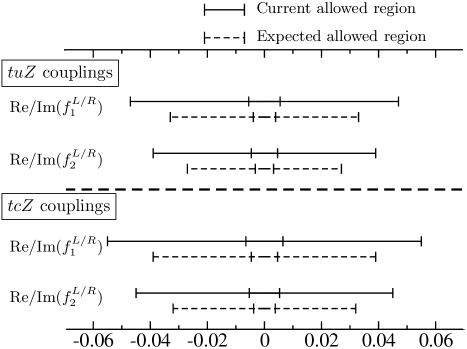
Figure 1: Current and expected constraints on the $tuZ$ and $tcZ$ couplings: The solid (dashed) lines mean the current (expected) allowed ranges for $tuZ$ and $tcZ$ shown in Tables 3. Numerical analyses and 3. Numerical analyses ( Eqs.(6) and (7) ). The region between the two inside bars on each line is derived using ${\mit\Gamma}_{tuZ}=8.1\times 10^{-6}(4.1\times 10^{-6})$, ${\mit\Gamma}_{tcZ}=1.1\times 10^{-5}(5.5\times 10^{-6})$ and that between the two outside bars is derived using ${\mit\Gamma}_{tuZ}=5.9\times 10^{-4}(3.0\times 10^{-4})$, ${\mit\Gamma}_{tcZ}=8.0\times 10^{-4}(4.0\times 10^{-4})$.

• Current constraints (compare with Tables 3. Numerical analyses and 3. Numerical analyses)

  • $tuZ$ couplings —Re/Im(f_1^L/R)—≤2.9×10^-2,   —Re/Im(f_2^L/R)—≤2.4×10^-2

  • $tcZ$ couplings —Re/Im(f_1^L/R)—≤3.4×10^-2,   —Re/Im(f_2^L/R)—≤2.8×10^-2

• Expected constraints (compare with Eqs.(6) and (7))

  • $tuZ$ couplings —Re/Im(f_1^L/R)—≤2.0×10^-2,   —Re/Im(f_2^L/R)—≤1.7×10^-2

  • $tcZ$ couplings —Re/Im(f_1^L/R)—≤2.4×10^-2,   —Re/Im(f_2^L/R)—≤2.0×10^-2

Thus, even if the present experimental ${\mit\Gamma}^{t}$ is replaced with the standard-model prediction and the uncertainty is neglected, rather large non-standard coupling constants still could exist. Note however that two (or more) non-standard couplings among the rest are needed to take large values at the same time in this case in order to balance out the contribution from each non-standard coupling.

4. Summary

We have here provided allowed regions of the non-standard $tuZ$ and $tcZ$ couplings via the recent experimental limits of Br($t\to uZ$) and Br($t\to cZ$) based on the effective-Lagrangian approach. In this analysis, we treated all the non-standard couplings as complex numbers which can vary independently of each other and gave constraints on them. It was found that the current allowed regions of these coupling are relatively large even if we use the standard-model ${\mit\Gamma}^{t}$ and neglect its uncertainty because their contributions cancel out each other to a certain extent. It was also pointed out that the allowed regions derived here could get narrowed by about 30 % at the HL-LHC. This means that there are good chances of discovering some evidence of the FCNC on the top-quark sector at the HL-LHC, if some of the current minimum or maximum values of the non-standard couplings are close to the actual ones in nature.

 Acknowledgments

This work was partly supported by the Grant-in-Aid for Scientific Research (C) Grant Number 17K05426 from the Japan Society for the Promotion of Science. Part of the algebraic and numerical calculations were carried out on the computer system at Yukawa Institute for Theoretical Physics (YITP), Kyoto University.

References

- [1] G. Aad et al. [ATLAS Collaboration], Phys. Lett. B 716 (2012) 1 (arXiv:1207.7214 [hep-ex]).
- [2] S. Chatrchyan et al. [CMS Collaboration], Phys. Lett. B 716 (2012) 30 (arXiv:1207.7235 [hep-ex]).
- [3] M. Russell, Ph.D. thesis, Glasgow U. (2017) (arXiv:1709.10508 [hep-ph]).
- [4] S.L. Glashow, J. Iliopoulos and L. Maiani, Phys. Rev. D 2 (1970) 1285.
- [5] I.I.Y. Bigi and H. Krasemann, Z. Phys. C 7 (1981) 127.
- [6] I.I.Y. Bigi, Y.L. Dokshitzer, V.A. Khoze, J.H. Kuhn and P.M. Zerwas, Phys. Lett. B 181 (1986) 157.
- [7] J.A. Aguilar-Saavedra, Acta Phys. Polon. B 35 (2004) 2695 (hep-ph/0409342).
- [8] T. Han, R.D. Peccei and X. Zhang, Nucl. Phys. B 454 (1995) 527 (hep-ph/9506461).
- [9] T. Han and J.L. Hewett, Phys. Rev. D 60 (1999) 074015 (hep-ph/9811237).
- [10] F. del Aguila, J.A. Aguilar-Saavedra and L. Ametller, Phys. Lett. B 462 (1999) 310 (hep-ph/9906462).
- [11] F. del Aguila and J.A. Aguilar-Saavedra, Nucl. Phys. B 576 (2000) 56 (hep-ph/9909222).
- [12] F. Larios, R. Martinez and M.A. Perez, Phys. Rev. D 72 (2005) 057504 (hep-ph/0412222).
- [13] F. Larios, R. Martinez and M.A. Perez, Int. J. Mod. Phys. A 21 (2006) 3473 (hep-ph/0605003).
- [14] R.A. Coimbra, P.M. Ferreira, R.B. Guedes, O. Oliveira, A. Onofre, R. Santos and M. Won, Phys. Rev. D 79 (2009) 014006 (arXiv:0811.1743 [hep-ph]).
- [15] J. Drobnak, S. Fajfer and J.F. Kamenik, JHEP 0903 (2009) 077 (arXiv:0812.0294 [hep-ph]).
- [16] P.M. Ferreira and R. Santos, Phys. Rev. D 80 (2009) 114006 (arXiv:0903.4470 [hep-ph]).
- [17] A. Datta and M. Duraisamy, Phys. Rev. D 81 (2010) 074008 (arXiv:0912.4785 [hep-ph]).
- [18] R. Goldouzian, Phys. Rev. D 91 (2015) 014022 (arXiv:1408.0493 [hep-ph]).
- [19] H. Khanpour, S. Khatibi, M. Khatiri Yanehsari and M. Mohammadi Najafabadi, Phys. Lett. B 775 (2017) 25 (arXiv:1408.2090 [hep-ph]).
- [20] G. Durieux, F. Maltoni and C. Zhang, Phys. Rev. D 91 (2015) 074017 (arXiv:1412.7166 [hep-ph]).
- [21] J.A. Aguilar-Saavedra, Eur. Phys. J. C 77 (2017) 769 (arXiv:1709.03975 [hep-ph]).
- [22] J.F. Shen, Y.Q. Li and Y.B. Liu, Phys. Lett. B 776 (2018) 391 (arXiv:1712.03506 [hep-ph]).
- [23] W. Buchmuller and D. Wyler, Nucl. Phys. B 268 (1986) 621.
- [24] C. Arzt, M.B. Einhorn and J. Wudka, Nucl. Phys. B 433 (1995) 41 (hep-ph/9405214).
- [25] J.A. Aguilar-Saavedra, Nucl. Phys. B 812 (2009) 181 (arXiv:0811.3842 [hep-ph]).
- [26] B. Grzadkowski, M. Iskrzynski, M. Misiak and J. Rosiek, JHEP 1010 (2010) 085 (arXiv:1008.4884 [hep-ph]).
- [27] M. Aaboud et al. [ATLAS Collaboration], Eur. Phys. J. C 78 (2018) 129 (arXiv:1709.04207 [hep-ex]).
- [28] The ATLAS collaboration , ATLAS-CONF-2017-070.
- [29] M. Tanabashi et al. [ParticleDataGroup], Phys. Rev. D 98 (2018) 030001.
- [30] CMS Collaboration, CMS-PAS-FTR-13-016.
- [31] J. Gao, C.S. Li and H.X. Zhu, Phys. Rev. Lett. 110 (2013) 042001 (arXiv:1210.2808 [hep-ph]).