Implementation of the exact semi-classical light-matter interaction - the easy way

Abstract

We present an analytical and numerical solution of the calculation of the transition moments for the exact semi-classical light-matter interaction for wavefunctions expanded in a Gaussian basis. By a simple manipulation we show that the exact semi-classical light-matter interaction of a plane wave can be compared to a Fourier transformation of a Gaussian where analytical recursive formulas are well known and hence making the difficulty in the implementation of the exact semi-classical light-matter interaction comparable to the transition dipole. Since the evaluation of the analytical expression involves a new Gaussian we instead have chosen to evaluate the integrals using a standard Gauß-Hermite quadrature since this is faster. A brief discussion of the numerical advantages of the exact semi-classical light-matter interaction in comparison to the multipole expansion along with the unphysical interpretation of the multipole expansion is discussed. Numerical examples on [CuCl₄]^2- to show that the usual features of the multipole expansion is immediately visible also for the exact semi-classical light-matter interaction and that this can be used to distinguish between symmetries. Calculation on [FeCl₄]^1- is presented to demonstrate the better numerical stability with respect to the choice of basis set in comparison to the multipole expansion and finally Fe-O-Fe to show origin independence is a given for the exact operator. The implementation is freely available in OpenMolcas.

I Introduction

Over the years a large variety of spectroscopies has been developed which has given a great understanding of molecules and materials from basic characterization edited by J. Lindon and Koppenaal (2016). All spectroscopies, until recently Abbott et al. (2016), all come from the interaction between external or internal electromagnetic fields. While a great deal of information can be extracted from experimental spectra alone, the more detailed correspondence between observed properties and molecular structures is often better illuminated when experimental results are combined with theoretical results since individual transitions can be separated.

In reconstructing the experimental spectra from theory it is necessary to introduce the given external electromagnetic fields in the description of the molecular system. The external fields used in the different types of spectroscopy are often weak in comparison to the atomic fields, or does not significantly perturb the system before measurement, and can therefore be treated classically (2006) (Ed.); Joachain et al. (2000); Posthumus (2004) and as a perturbation. Usually, for laser fields, the electromagnetic field is described by a plane wave where the wave vector is a complex exponential function. Traditionally a multipole expansion is introduced and truncated at some finite order to describe the interaction of the external electromagnetic field with the system. The first term in this multipole expansion is the electric dipole, and the next term that is included is typically the electric quadrupole, followed by other magnetic and electric multipoles. While simple, the higher order terms depend on the choice of origin for the multipole expansion, at least in cases where there are non-zero terms of lower order. For weak fields, which can be treated as a perturbation, the problem of origin dependence was recently solved by Bernadotte et al. Bernadotte et al. (2012) simply by truncating the multipole in the observable wave vector and not in the non-observable transition moments traditionally done. A complete expansion to the second order, most commonly associated with electric quadrupole, then requires calculations up to magnetic quadruples and electric octupoles.

Bernadotte et al. Bernadotte et al. (2012) showed that origin dependence is exact when using the velocity gauge. We later showed that origin independence in a finite basis set can also be accomplished in the length gauge but what is typically referred to as the length gauge is actually a mixed gauge, with the electric and magnetic components in the length and velocity gauges respectively.Sørensen et al. (2017a) Origin independence, in finite basis sets, is not conserved in this mixed gauge.Sørensen et al. (2017b) Furthermore the increased basis set requirement and convergence behaviour for every order in the multipole expansion cannot be overlooked Crossley (1969); Sørensen et al. (2017b).

An alternative way to evaluate the oscillator strengths is to simply use the exact semi-classical light-matter interaction and not perform any multipole expansion. In this way there will only be one type of integrand that needs to be evaluated and not, like for the multipole expansion, many integrands with different basis sets requirements. Exact semi-classical light-matter interactions of a plane wave have been implemented previously.Lehtola et al. (2012); List et al. (2015, 2017) The evaluation of the integrals for the exact semi-classical light-matter interaction has been the major obstacle in the evaluation of the operator and often described as being very difficult Lehtola et al. (2012); Bernadotte et al. (2012). Either a number of new recursive relations needs to be programmed along with the need to introduce trigonometric functionsList et al. (2015, 2017) or a Fourier transformation of the overlap between basis function should be performed.Lehtola et al. (2012) We, however, intend to show that the evaluation of the integrals for the exact semi-classical light-matter interaction in a Gaussian basis set is actually very simple and can be performed using either analytical formulas or standard integral evaluation methods in quantum chemistry.

To illustrate the behavior of the exact operator we will perform calculations with high-energy photons, which corresponds to large k vectors, rapidly oscillating fields, and thus larger relative intensity of higher-order terms in the plane-wave expansion. In X-ray absorption spectroscopy (XAS), the K-edge of first-row transition metals, typically associated with electric dipole-allowed $1s$ to $4p$ transitions, uses photon energies of thousands of eV. Before the rising edge, there are weaker pre-edge transitions assigned to $1s$ to $3d$ transitions, which provides insight into the nature of the bonding between the transition metal(s) and ligands.Shulman et al. (1976); Hahn et al. (1982); Westre et al. (1997) Since the $1s$ to $3d$ is dipole forbidden in centrosymmetric environments, higher-order terms in the multipole expansion must be included in order to describe these transitions, or by using the exact operator.List et al. (2017)

The X-ray calculations will be performed using the restricted active space (RAS) method, which is a multiconfigurational wavefunction approach.Olsen et al. (1988); Malmqvist et al. (1990) RAS has been successfully applied to simulate L-edge XAS and resonant inelastic X-ray scattering (RIXS) of several transition metal systems.Josefsson et al. (2012); Bokarev et al. (2013); Pinjari et al. (2014) We have also implemented the second-order expansion of the wave vector to describe XAS and resonant inelastic X-ray scattering (RIXS) in the K pre edge.Guo et al. (2016a, b)

The presented examples all represent cases with weak electromagnetic fields. However, in the past decades with advent of very short and brilliant laser pulses the perturbative treatment can break down in and one enters the strong field regime where the external and atomic field must treated on equal footing and a dynamical treatment is necessary (2006) (Ed.); Joachain et al. (2000); Posthumus (2004). For strong fields, beyond the dipole approximation, the problem of origin dependence still persists for the multipole expansion. We will here allude to how the work on the exact semi-classical light-matter interaction can be carried directly over to the strong field regime because all interaction terms can be evaluated using the same simple integrals. This also means that the method also could be used in simulations of dynamics of molecules in strong electric and magnetic fields and this, we believe, is where the real strength of the approach may lie.

For self consistency we will in Sec. II.1 recapitulate the perturbative treatment of molecules in weak electromagnetic fields and the multipole expansion. Thereafter in Sec. II.2 we will show how the integrals for the exact semi-classical light-matter interaction can be evaluated using standard quantum chemistry integral programs. Followed by the isotropically averaged oscillator strengths in Sec. II.2.1 For the applications in Sec. III we demonstrate the advantage of using the exact semi-classical light-matter interaction instead of the multipole expansion on different systems which has been problematic with the multipole-expansion approach. A perspective on and the possibility of dynamics simulations with the exact semi-classical light-matter interaction is given in Sec. IV.1 and finally a summary and conclusion in Sec V.

II Theory

In the first of the two parts of this section we will briefly discuss the well-known formulas for the semi-classical light-matter interaction and how the oscillator strengths usually are calculated from perturbation theory along with a short discussion of the unphysical interpretation of the multipole expansion often seen. In the second part we will show the integrals for the exact semi-classical light matter interaction can be evaluated analytically along with an easy way to compute the integrals using a standard Gauß-Hermite quadrature. Finally the isotropic averaging of the exact semi-classical light matter interaction is mentioned.

II.1 Perturbation from weak fields

Throughout this section it is assumed that the electromagnetic fields are weak and therefore can be treated as a perturbation of the molecular system. The zeroth order Hamiltonian, in our case, is the Schrödinger equation within the Born-Oppenheimer approximation

$$\hat{H}_{0}=\sum_{i=1}^{N}\frac{\bm{\hat{p}}_{i}^{2}}{2m_{e}}+V(\bm{r}_{1},\ldots,\bm{r}_{N})$$ (1)

which is exposed to a time-dependent perturbation $\hat{U}(t)$

$$\hat{U}(t) = -\frac{e}{m_{e}c}\sum_{i}\bm{A(r}_{i},t)\bm{\cdot\hat{p}}_{i}+\frac{e^{2}}{2m_{e}c^{2}}\bm{A^{2}(r}_{i},t)-\frac{ge}{2m_{e}c}\sum_{i}\bm{B(r}_{i},t)\bm{\cdot\hat{s}}_{i}$$ (2)

$$= \frac{eA_{0}}{2m_{e}c}\sum_{i}\Big{[}exp(\imath(\bm{k\cdot r}_{i}-\omega t))(\bm{\mathcal{E}\cdot\hat{p}}_{i})$$ (3)

$$+ \frac{eA_{0}}{4c}(exp(2\imath(\bm{k\cdot r}_{i}-\omega t))+1)$$ (4)

$$+ \imath\frac{g}{2}exp(\imath\bm{k\cdot r}_{i}-\omega t)(\bm{k\times\mathcal{E}})\cdot\bm{\hat{s}}_{i}+c.c.\Big{]}$$ (5)

from a monochromatic linearly polarized electromagnetic wave where $\bm{k}$ is the wave vector pointing in the direction of propagation, $\bm{\mathcal{E}}$ the polarization vector perpendicular to $\bm{k}$, $\omega$ is the angular frequency, $\bm{\hat{s}}$ the spin and $A_{0}$ the amplitude of the vector potential.

Of the terms in Eqs. 3-5 often the dipole approximation is taken meaning that only the zeroth order term in the vector potential $(\bm{A})$ in Eq. 3 is included

$$exp(\imath\bm{k\cdot r}_{i})=1+\imath(\bm{k\cdot r}_{i})-\frac{1}{2}(\bm{k\cdot r}_{i})^{2}+\ldots$$ (6)

While the dipole approximation suffices for optical transitions for analyzing the K-edge in X-ray spectroscopy terms up to second order must be included. The $(\bm{A}^{2})$ in Eq. 4 is mostly relevant for strong fields and will always depend explicitly on the field strength $A_{0}$ which makes little sense for weak fields, treated perturbatively, where this dependence is removed from the terms in Eqs. 3 and 5. Eq. 5 describes the interaction between the spin and the magnetic field and is relevant when describing open shell transitions. Furthermore the values of all terms in Eqs. 3-5 also depend on the choice of gauge, though the sum is constant. In the Coulomb gauge, which is the usual choice in molecular physics, $(\bm{A}^{2})$ has a minimum Gubarev et al. (2001) and will be neglected in the applications.

Using Fermi’s golden rule transitions only occur when the energy difference between the eigenstates of the unperturbed molecule matches the frequency of the perturbation

$$\omega=\omega_{0n}=\frac{E_{n}-E_{0}}{\hbar}$$ (7)

and the explicit time dependence can be eliminated from the transition rate

$$\Gamma_{0n}(\omega)=\frac{2\pi}{\hbar}|\langle 0|\hat{U}|n\rangle|^{2}\delta(\omega-\omega_{0n})=\frac{\pi A_{0}^{2}}{2\hbar c}|T_{0n}|^{2}\delta(\omega-\omega_{0n})$$ (8)

and the effect of the weak electromagnetic field can now be expressed as a time-independent expectation value. From Eq. 8 the relation between the transition moments $T_{0n}$ and the time-independent part of $\hat{U}$ in Eq. 2 is seen. From the transition moments $T_{0n}$ the oscillator strengths $f_{0n}$

$$f_{0n}=\frac{2m_{e}}{e^{2}E_{0n}}|T_{0n}|^{2},$$ (9)

where $E_{0n}=E_{n}-E_{0}$ is the difference in the energy of the eigenstates of the unperturbed molecule, can then be calculated. The amplitude of the electric and magnetic field $E_{0}=B_{0}=A_{0}k$ or intensity therefore does not have to be defined for Eqs. 3 and 5 while for the quadratic $\boldmath{A}$ term in Eq. 4 the amplitude is still needed.

Traditionally a multipole expansion of the exponential function of the perturbation in Eq. 2 is performed which gives rise to the non-observable electric and magnetic dipole, quadrupole and higher order approximations for the transition moments $T_{0n}$. Unfortunately such an expansion in the transition moments $T_{0n}$ is only origin independent for the dipole and in the limit of a complete expansion.

Origin independence, however, appears naturally provided that the collection of the terms in Taylor expansion of the exponential of the wave vector $k$ in Eq. 2 are collected to the same order in the observable oscillator strengths

$$f_{0n}=f_{0n}^{(0)}+f_{0n}^{(1)}+f_{0n}^{(2)}+\ldots=\frac{2m_{e}}{e^{2}E_{0n}}|T_{0n}^{(0)}+T_{0n}^{(1)}+T_{0n}^{(2)}+\ldots|^{2}$$ (10)

as shown by Bernadotte et al. Bernadotte et al. (2012). Lestrange et al. J. Lestrange et al. (2015) demonstrated that collecting the terms in the oscillator strengths according to Eq. 10 does not always ensure a positive total oscillator strength when truncating the expansion since the perfect square of the transition moments is broken. The total negative oscillator strengths when truncating Eq. 10 appear to be a basis set problem that can occur for unbalanced basis sets for some transitions Sørensen et al. (2017b).

While the truncation in the oscillator strength eliminates the problem of origin dependence the multipole expansion, however, introduces an increasing demand on the basis set for every order in the expansion since the integrand changes for every order Crossley (1969). This means that in order to calculate the K pre-edge peaks in an X-ray spectrum the basis set must be able to accurately describe all terms at least up to second order in the transition moment i.e., the electric octupole and magnetic quadrupole terms. While the higher order terms could be expected to be small these can be grossly overestimated in some basis sets Sørensen et al. (2017b).

Lastly, none of the terms in the multipole expansion in Eq. 10 are individually observable so there is no physical argument to perform and try to interpret the expansion except that this is what is historically done. The same argument also goes for the origin independent oscillator strength Bernadotte et al. (2012) which despite the origin independence still are not individually observable. Therefore trying to interpret spectra in terms of the different orders in the multipole expansion or even as electric or magnetic is completely unphysical since only the total can be observed and changes of coordinate system can significantly alter the interpretation Sørensen et al. (2017b).

II.2 Evaluation of the integrals for the exact semi-classical light-matter interaction

The evaluation of the integrals for the exact semi-classical light-matter interaction has been the major obstacle in the evaluation of the operator.Lehtola et al. (2012); Bernadotte et al. (2012) We will show that the exact semi-classical light-matter interaction of a plane wave can be thought of as a Fourier transformation of the overlap between basis functions and that this can be solved analytically. In the Gaussian basis sets we use this just results in a new Fourier-transformed Gaussian. The evaluation of the integrals are therefore very similar to those found for the overlap and operators in a Gaussian Planewave basis set Polášek and Čarsky (2002); Čarsky and Polášek (1998); Füsti-Molnar and Pulay (2002) and similarities are shared with the plane wave representations of the electromagnetic field Devaney and Wolf (1974).

In order to evaluate Eq. 8 for the perturbation in Eq. 2 the matrix element

$$\langle 0|\hat{U}|n\rangle=\sum_{\mu\nu}U_{\mu\nu}^{AB}\gamma_{\mu\nu}^{AB}$$ (11)

must be calculated. In Eq. 11 $U_{\mu\nu}^{AB}$ is the integral matrix for the orbital bases $A$ and $B$ with indices $\mu$ and $\nu$ and likewise defined for the transition density matrix $\gamma_{\mu\nu}^{AB}$ Malmqvist (1986). For a wave function expanded in Gaussians the individual terms in $U_{\mu\nu}^{AB}$ from Eq. 3 correspond to evaluating integrals of the form

$$I=\langle\chi_{\mu}|e^{\pm\imath\bm{k\cdot r}}\bm{\hat{p}}|\chi_{\nu}\rangle\bm{\cdot\mathcal{E}}$$ (12)

where the real-valued atomic Cartesian basis functions $\chi_{\mu}$ and $\chi_{\nu}$ are expressed as

$$\chi_{\mu}(\bm{r}) = \chi_{i,j,k}(\bm{r},\alpha_{\mu},\bm{A})$$ (13)

$$= (x-A_{x})^{i}(y-A_{y})^{j}(z-A_{z})^{k}e^{-\alpha_{\mu}\|\bm{r}-\bm{A}\|^{2}}$$ (14)

$$= \chi_{i}(x,\alpha_{\mu},A_{x})\chi_{j}(y,\alpha_{\mu},A_{y})\chi_{i}(z,\alpha_{\mu},A_{z})$$ (15)

in their different components, where $i$, $j$, and $k$ represent the order of the Cartesian components $x$, $y$, and $z$, respectively. The integral in Eq. 12 can be factorized into three one-dimensional integrals

$$I_{x}=\int_{-\infty}^{\infty}\chi_{i}(x,\alpha_{\mu},A_{x})e^{\pm\imath k_{x}x}\epsilon_{x}\hat{p}_{x}\chi_{j}(x,\alpha_{\nu},B_{x})dx.$$ (16)

Applying the differentiation operator $\hat{p}_{x}=-\imath\hbar\frac{\partial}{\partial x}$ we find

$$I_{x}=-\imath\hbar\epsilon_{x}\int_{-\infty}^{\infty}\chi_{i}(x,\alpha_{\mu},A_{x})e^{\pm\imath k_{x}x}\left(j\chi_{j-1}(x,\alpha_{\nu},B_{x})-2\alpha_{\nu}\chi_{j+1}(x,\alpha_{\nu},B_{x})\right)dx$$ (17)

that the integral $I_{x}$ can be expressed as a sum of two terms. From Eq. 17 it is seen that both terms are of the form

$$\int_{-\infty}^{\infty}e^{\pm\imath k_{x}x}\chi_{i}(x,\alpha_{\mu},A_{x})\chi_{j}(x,\alpha_{\nu},B_{x}).$$ (18)

Using the Gaussian product formula we see that the expression in Eq. 18 is akin to a Fourier transformation of a Gaussian from real space $x$ to $k_{x}$ space. Integrals of the from in Eq. 18 can be solved analytically using recursive formulas for the analytical Fourier representation of Gaussians Polášek and Čarsky (2002). Eq. 18 can also be viewed as the Fourier transformation of the overlap between two basis functions as also noted by Lethola et al. Lehtola et al. (2012).

Since the Fourier transformation of a Gaussian is a new Gaussian we have chosen not to use the analytical form but instead rewrite the integral in Eq. 18 to a form which easily can be evaluated by a standard Gauß-Hermite quadrature. Using the Gaussian product formula on Eq. 18

$$I_{x}^{\prime} = \int_{-\infty}^{\infty}e^{\pm\imath k_{x}x}\chi_{i}(x,\alpha_{\mu},A_{x})\chi_{j}(x,\alpha_{\nu},B_{x})$$ (19)

$$= e^{-\frac{\alpha_{\mu}\alpha_{\nu}}{\zeta}(A_{x}-B_{x})^{2}}\int_{-\infty}^{\infty}(x-A_{x})^{i}(x-B_{x})^{j}e^{-\zeta(x-P_{x})^{2}\pm\imath k_{x}x}dx$$ (20)

where $\zeta=\alpha_{\mu}+\alpha_{\nu}$ and $P_{x}=(\alpha_{\mu}A_{x}+\alpha_{\nu}B_{x})/\zeta$ we can complete the square in the exponent

$$I_{x}^{\prime}=e^{-\frac{\alpha_{\mu}\alpha_{\nu}}{\zeta}(A_{x}-B_{x})^{2}}e^{\gamma}\int_{-\infty}^{\infty}(x-A_{x})^{i}(x-B_{x})^{j}e^{-\zeta(x-Q_{x})^{2}}dx$$ (21)

where $Q_{x}=P_{x}\pm\imath k_{x}/(2\zeta)$ and $\gamma=\zeta(Q_{x}^{2}-P_{x}^{2})$. We here notice that for mixed Gaussian Plane wave basis set expressions similar to Eq. 20 for an overlap appears Füsti-Molnar and Pulay (2002).

Making a change of variables $z=\sqrt{\zeta}(x-Q_{x})$ the integral in Eq. 21 can now be transformed to

$$I_{x}^{\prime}=\Theta\lim_{R\rightarrow\infty}\int_{-z=\sqrt{\zeta}(R-Q_{x})}^{z=\sqrt{\zeta}(R-Q_{x})}(\frac{z}{\sqrt{\zeta}}+Q_{x}-A_{x})^{i}(\frac{z}{\sqrt{\zeta}}+Q_{x}-B_{x})^{j}e^{-z^{2}}dz$$ (22)

where

$$\Theta=e^{-\frac{\alpha_{\mu}\alpha_{\nu}}{\zeta}(A_{x}-B_{x})^{2}}e^{\gamma}/\sqrt{\zeta}.$$ (23)

Defining the polynomial

$$f(z)=\Theta(\frac{z}{\sqrt{\zeta}}+Q_{x}-A_{x})^{i}(\frac{z}{\sqrt{\zeta}}+Q_{x}-B_{x})^{j}$$ (24)

Eq. 22 can be written a little more compact

$$I_{x}^{\prime}=\lim_{R\rightarrow\infty}\int_{-z=\sqrt{\zeta}(R-Q_{x})}^{z=\sqrt{\zeta}(R-Q_{x})}f(z)e^{-z^{2}}dz.$$ (25)

Since the integral in Eq. 25 is analytic the integration is independent of the path and can therefore be split into

$$I_{x}^{\prime} = \lim_{R\rightarrow\infty}\int_{-z=\sqrt{\zeta}(R-Q_{x})}^{z=\sqrt{\zeta}R}f(z)e^{-z^{2}}dz$$ (26)

$$+ \lim_{R\rightarrow\infty}\int_{-z=\sqrt{\zeta}R}^{z=\sqrt{\zeta}R}f(z)e^{-z^{2}}dz$$ (27)

$$+ \lim_{R\rightarrow\infty}\int_{-z=\sqrt{\zeta}R}^{z=\sqrt{\zeta}(R-Q_{x})}f(z)e^{-z^{2}}dz.$$ (28)

Since $\sqrt{\zeta}>0$ and the exponential decay of the integrand as $\mathfrak{R}_{z}\rightarrow\pm\infty$ two of the integrals vanishes leaving

$$I_{x}^{\prime}=\lim_{R\rightarrow\infty}\int_{-z=\sqrt{\zeta}R}^{z=\sqrt{\zeta}R}f(z)e^{-z^{2}}dz=\int_{-\infty}^{\infty}f(z)e^{-z^{2}}dz$$ (29)

for which the Gauß-Hermite quadrature is designed to compute. Since $z$ is complex the Gauß-Hermite quadrature must use complex numbers. With the standard Gauß-Hermite nodes $z_{n}$ and weights $w_{n}$, we compute the integral as

$$I_{x}^{\prime}=\sum_{n}w_{n}f(z_{n})$$ (30)

or equivalently with the transformed quadrature nodes $x_{n}=z_{n}/\sqrt{\zeta}+Q_{x}$

$$I_{x}^{\prime}=\Theta\sum_{n}w_{n}(x_{n}-A_{x})^{i}(x_{n}-B_{x})^{j}.$$ (31)

The total integral in Eq. 12 can therefore simply be written as

$$I=I_{x}^{\prime}*I_{y}^{\prime}*I_{z}^{\prime}.$$ (32)

Due to the similarities between the electric term in the exact semi-classical light-matter interaction for a plane wave (Eq. 3), with the quadratic and magnetic terms (Eqs. 4 and 5) all these integrals can be evaluated in exactly the same manner. All three terms are therefore programmed in OpenMolcas ”https://gitlab.com/Molcas/OpenMolcas” . The coupling between the magnetic field and the spin in Eq. 5 is only non-zero when the spin-orbit operator in the RASSI module Malmqvist et al. (2002) is used. Eq. 4 also gives a constant non-zero contribution in all directions but since Eq. 4 still depends explicitly on the field strength we have neglected this term since for the field strengths needed for Eq. 4 to be influential the perturbative treatment of the light-matter interaction will break down.

The resulting formulas are not surprisingly like those found using Rys quadrature in a Gaussian plane wave basis set as derived by Čarsky and Polášek Čarsky and Polášek (1998) and does not require any new recursive relations or expansion in trigonometric functions like previous implementations List et al. (2015, 2017).

II.2.1 Isotropically averaged oscillator strengths

For the terms in the multipole expansion well known isotropically tensor averaged oscillator strengths can be found in literature Barron (2004). For the exact expression no closed formula exists. Lebedev and co-workers Lebedev (1975, 1976, 1977); Lebedevand and Skorokhodov (1992); Lebedev (1995); Lebedevand and Laikov (1999) have devised a way of distributing quadrature points over a unit sphere defining a Lebedev grid which gives the propagation directions included in the numerical integration for the incoming light. By averaging over two orthogonal polarization directions for the different directions for the propagation the exact isotropic average can be systematically approximated. List et al. List et al. (2017) have shown that this converges very rapidly with the number of quadrature points and we therefore have also adopted the Lebedev grid for the isotropic averaging.

III Application

In this section we will study the metal K pre edge XAS of two molecular systems, [CuCl₄]^2- and [FeCl₄]^1-, as well as the iron dimer model complex [Fe₂O]⁴⁺, to highlight properties specific to the use of the exact semi-classical operator v.s. standard multipole techniques. In a classical experiment, the angular dependence of the pre-edge intensity of single-crystal [CuCl₄]^2- was used to identify the electric quadrupole contribution and to identify the symmetry of the singly-occupied 3d orbital. In general, the assignment of transitions to different multipole contributions has helped to connect spectra to the electronic structure. With the [CuCl₄]^2- example, we will demonstrate how the exact operator reproduces the behavior of what is traditionally referred to as an electric quadrupole transition.

As mentioned above, electric quadrupole transitions are origin-dependent if the electric dipole contributions are non-zero. [FeCl₄]^1- has tetrahedral symmetry, and the non-centrosymmetric ligand environment leads to intense dipole contributions and strong contributions from many terms in the full second-order expansion.Bernadotte et al. (2012); Guo et al. (2016a); Sørensen et al. (2017b) For some basis sets, the expansion even leads to unphysical negative oscillator strengths.J. Lestrange et al. (2015); Sørensen et al. (2017b, a) These examples are revisited with the exact semi-classical operator to show its stability in incomplete basis sets.

Finally, we address an iron dimer where there is no natural choice of the origin for the multipole expansion of an iron-centered transition. We show the origin independence of the exact operator by comparing the results for [Fe₂O]⁴⁺ to previous calculations using the multipole expansion in the mixed gauge. However, before that we describe the computational details.

III.1 Computational details

The geometry of the [CuCl₄]^2- is taken from the X-ray crystal structure.Hahn et al. (1982) The complex has a square planar geometry, formal D₂h symmetry, with Cu-Cl bond lengths of 2.233 and 2.268 Å and Cl-Cu-Cl angles of 89.91^∘ and 90.09^∘. The short bonds were placed along the x-axis. To show the effect of the angles, another calculation in D_2h symmetry with Cl-Cu-Cl angles of 90^∘ and with all bonds along the x- and y-axis, here labelled D_2h⟂, were also performed. Finally, calculations were made in D_4h symmetry using an average bond length of 2.2505 Å.

The geometry of [FeCl₄]^1- is also taken from an X-ray structure.Warnke et al. (2010) The ligand environment is tetrahedral ($T_{d}$ point group) with four Fe-Cl distances of 2.186 Å. The geometry of Fe-O-Fe is taken from a BP86/6-311(d) geometry optimization of [(hedta)FeOFe(hedta)], which gives $C_{2v}$ symmetry, Fe-O distances of 1.76 Å and an angle of 148 degrees.Sørensen et al. (2017b)

Orbital optimization is performed using state-average RASSCF, with separate optimizations for ground and core-excited states as implemented in OpenMolcas.”https://gitlab.com/Molcas/OpenMolcas” In all calculations the metal 1s orbitals are included in RAS1, constraining to at most one hole. For the calculations of the core-excited states, the weights of all configurations with fully occupied 1s orbitals have been set to zero. To avoid orbital rotation, i.e., the hole appears in a higher-lying orbital, the 1s orbitals have been frozen in the calculation of the final states.

[CuCl₄]^2- is a formal 3d⁹ complex with a singly occupied 3d_x2-y2 orbital, leading to a doublet ground state. We focus only on the 1s$\rightarrow$3d_x2-y2 transition and use a small RAS2 space including seven electrons in four metal-centered orbitals, see Figure 1. Due to weak spin-orbit coupling, only final states of the same spin multiplicity as the ground state are considered in the calculations. For [CuCl₄]^2- only one doublet core excited state is necessary to include.

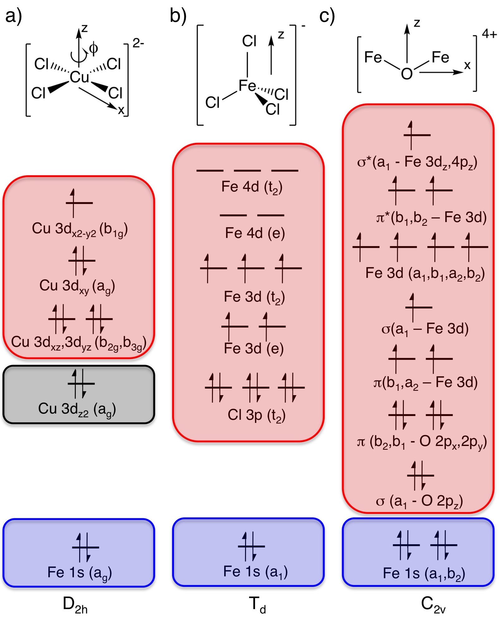
Figure 1: Ligand geometries and active spaces for metal K pre-edge XAS modeling of a) [CuCl₄]^2-, b) [FeCl₄]^1-, and c) [Fe₂O]⁴⁺.

[FeCl₄]^1- is a high-spin 3d⁵ complex with a sextet ground state. The calculations are similar to those laid out in previous works,Sørensen et al. (2017b, a) with eleven electrons in 13 orbitals in RAS2, see Figure 1. The orbitals of the sextet excited states were averaged over 70 states.

The ground state of the iron dimer [Fe₂O]⁴⁺ is an singlet, with five unpaired electrons on each ferric iron coupled antiferromagnetically. To facilitate RASSCF convergence, calculations are instead performed with ferromagnetic coupling, giving undectet states. The RAS2 space consists of the three 2p orbitals of the bridging oxygen and the ten 3d orbitals of the irons, which gives a total of 16 electrons in 13 orbitals, see Figure 1. 60 core-excited states were used, exactly like in previous work.Sørensen et al. (2017b)

For the correlation treatment all calculations will be at the RASSCF level as inclusion of dynamical correlation on the behavior of the transitions can be assumed to be minor. Scalar relativistic effects have been included by using a second-order Douglas-Kroll-Hess Hamiltonian in combination with the ANO-RCC-VTZP basis set.Douglas and Kroll (1974); Heß (1986); Roos et al. (2005, 2004) This basis set have been shown to perform reasonably well for both electronic structure and for the transition moments.Sørensen et al. (2017b) The intensities for the exact operator and the quadrupole intensities in the mixed gauge are implemented in the RASSI program Malmqvist and Roos (1989); Malmqvist et al. (2002) and distributed freely in the OpenMolcas package”https://gitlab.com/Molcas/OpenMolcas” . Simulated spectra are plotted using a Lorentzian lifetime broadening with a full-width-at-half-maximum (FWHM) of 1.25 eV and further convoluted with a Gaussian experimental broadening of 1.06 eV.

III.2 Assignment of K pre edge XAS contributions for [CuCl₄]^2-

Metal K pre-edges are weak transitions on the low-energy side of the rising edge. They are typically assigned to 1s$\rightarrow$3d transitions. In centrosymmetric geometries these are electric dipole forbidden and only gain intensity through what is typically referred to as electric quadrupole transitions. However, vibronic coupling with normal modes that break centrosymmetry allows for electric dipole contributions also for complexes with formal centrosymmetry.

In single crystals the orientation of the molecule with respect to the beam can be controlled. The angular dependence of the normalized peak heights in the Cu K pre edge of [CuCl₄]^2-, taken from reference Hahn et al. (1982), is shown in Figure 2a. The angle $\phi$ shows rotation around the molecular z-axis, with 0^∘ representing the direction of the electromagnetic k vector relative the short Cu-Cl bond. The electric quadrupolar contribution is distinguished by a four-fold periodicity of the cross section. The highest intensity is observed for orientations bisecting the Cu-Cl bond, which makes it possible to assign the half-filled orbital to be 3d_x2-y2.Hahn et al. (1982) The isotropic contribution is assigned to an electric dipole contribution that gains intensity through vibronic coupling.

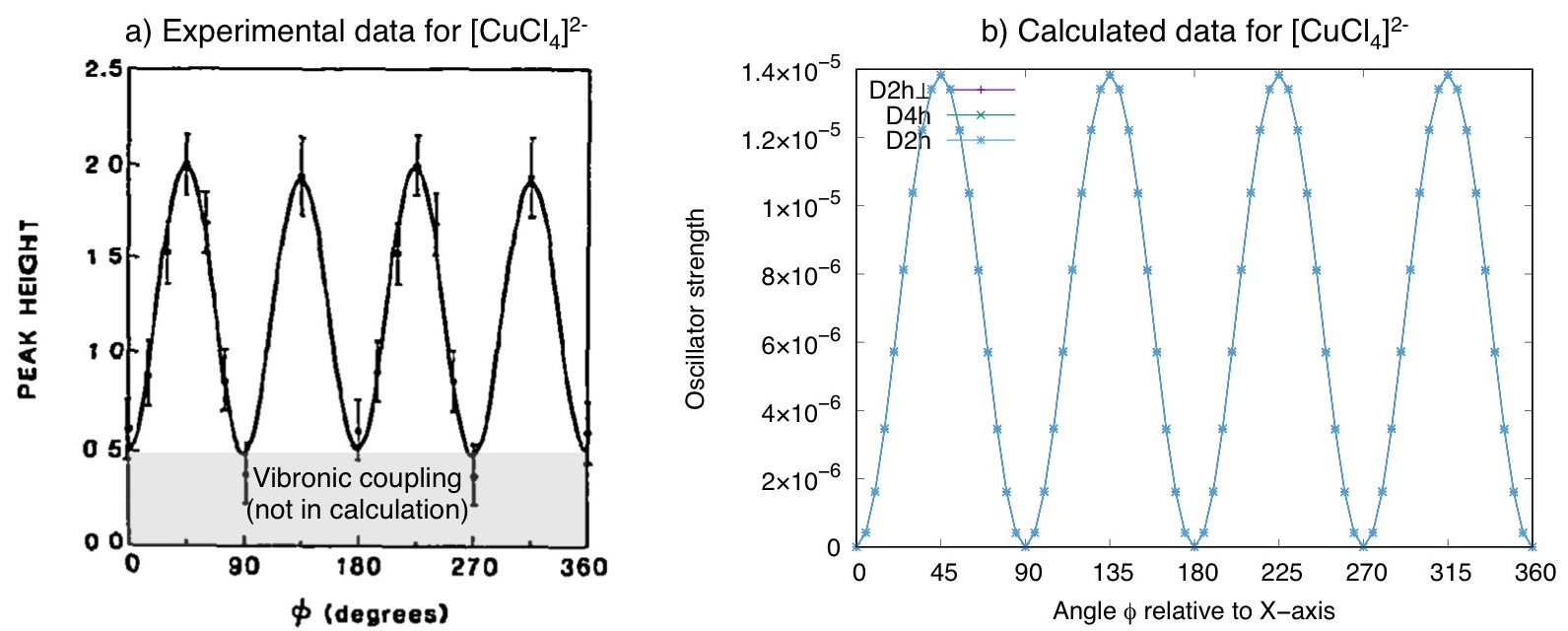
Figure 2: Experimental and calculated angular dependence of the K pre-edge transition in [CuCl₄]^2-. a) Normalized K pre-edge peak heights from reference Hahn et al. (1982). Reproduced with permission from b) Oscillator strengths calculated using the exact semi-classical light-matter interaction in different in with different symmetries.

The angular dependence of the oscillator strengths calculated using the exact operator is shown in Figure 2b. The four-fold periodicity is reproduced, which is a simple illustration that the exact operator reproduces the observables that have been traditionally used to assign transitions to different multipole components. The isotropic contributions are missing from the calculated spectra simply because vibronic coupling is not taken into account in our calculations.

In the real complex the Cu-Cl bonds are not perfectly symmetric. In order to see the very slight asymmetry in the angular spectrum of [CuCl₄]^2- one needs to explicitly compare the oscillators strengths on both sides of the peaks, e.g., 130^∘ and 140^∘. Due to the lack of data points and reasonably large error bars in the experiment distortions from D_4h are difficult to quantify in the experimental spectrum. In Table 1 the peak and minimum along with their neighboring values are listed to show the asymmetry in the spectrum of [CuCl₄]^2- is and how little the values changes with nuclear geometry. From Table 1 it is seen that the difference between the points next to the peak and minimum is a mere $1.0*10^{-8}$ for D_2h which of course is much lower than the accuracy of the calculation but still above numerical noise. For D_4h and the difference between symmetrically placed points is negligible and a numerical zero is observed at 90^∘ as it should be. Comparing the values for D_2h, D_4h and D_2h⟂ directly the difference is still below the accuracy of the calculation and discerning between D_4hand D_2h⟂ is not possible with the geometry differences here chosen.

Angle	D2h	D4h	D2h⟂
130	0.13423083E-04	0.13417817E-04	0.13415988E-04
135	0.13832984E-04	0.13834993E-04	0.13833106E-04
1400	0.13408657E-04	0.13417818E-04	0.13415986E-04
175	0.40993408E-06	0.41717685E-06	0.41711848E-06
180	0.32151105E-10	0.16725576E-17	0.10545833E-16
185	0.42435937E-06	0.41717540E-06	0.41711978E-06

Table 1: The oscillator strength around 45^∘ and 90^∘ for [CuCl₄]^2- in different symmetries.

III.3 Stability of K pre edge XAS intensities of [FeCl₄]^1-

[FeCl₄]^1- has a tetrahedral ligand environment. In T_d symmetry, the metal 3d orbitals belong to the $e$ and $t_{2}$ irreducible representations, see Figure 1. The iron 4p orbitals also have $t_{2}$, which means that they can mix through the interactions with the Cl ligands. The first two pre edge transitions are to the 3d($e$) orbitals, and are electric dipole forbidden. The next three are to the $t_{2}$ orbitals, and they are more intense as they are electric-dipole allowed through the 4p mixing and get large contributions from several orders in the multipole expansion.Westre et al. (1997); Guo et al. (2016a); Sørensen et al. (2017b) Not only will the electric quadrupole $f_{0n}^{(Q^{2})}$ term be large but the electric dipole $f_{0n}^{(\mu^{2})}$ will be very large and the electric dipole electric octupole $f_{0n}^{(\mu O)}$ term will also be significant even when the coordinate system is placed on the Fe atom.

In previous applications that examined the origin independence of the multipole expansion in a mixed gauge certain transitions in [FeCl₄]^1- gave negative oscillator strengths at the second order despite the fact that the zeroth order in the multipole expansion of the oscillator strengths should be the dominant term.Sørensen et al. (2017b) The strong negative oscillator strengths, however, only appeared in the cc-pVDZ and AUG-cc-pVDZ basis sets but not in the ANO-RCC basis sets. Since the oscillator strengths for the exact operator is inherently positive it would therefore be interesting to see what values the multipole expansion should converge to, and second, to make a comparison of the numerical stability and performance of the exact operator and the multipole expansion.

In Table 2 the total dipole, quadrupole and exact intensities for the transition from the ground to selected core-excited states in $[FeCl_{4}]^{1-}$ is shown in the ANO-RCC-VTZP and AUG-cc-pVDZ basis sets. The $G\rightarrow C1$ transition reaches the 3d($e$) orbital, while both C3 and C5 are 3d($t_{2}$) final states. C12 is a two-electron excitations, with both core and valence electrons excited simultaneously, and are typically weaker than the main transitions.

Basis	Transition	$f_{0n}^{(\mu^{2})}$	$f_{0n}^{(\mu^{2})^{p}}$	$f_{0n}^{(2)}$	Total	Exact
ANO-RCC-VTZP	$G\rightarrow C1$	0.157E-12	0.151E-12	0.407E-05	0.407E-05	0.371E-05
AUG-cc-pVDZ	$G\rightarrow C1$	0.765E-06	0.447E-06	0.258E-05	0.335E-05	0.472E-05
ANO-RCC-VTZPSørensen et al. (2017b)	$G\rightarrow C3$	0.283E-04	0.273E-04	0.144E-05	0.427E-04	0.305E-04
AUG-cc-pVDZSørensen et al. (2017b)	$G\rightarrow C3$	0.281E-04	0.168E-04	-0.585E-04	-0.304E-04	0.209E-04
ANO-RCC-VTZP	$G\rightarrow C5$	0.283E-04	0.273E-04	0.144E-05	0.427E-04	0.305E-04
AUG-cc-pVDZ	$G\rightarrow C5$	0.234E-04	0.169E-04	-0.539E-04	-0.305E-04	0.210E-04
ANO-RCC-VTZP	$G\rightarrow C12$	0.555E-09	0.419E-09	-0.353E-09	0.202E-09	0.484E-09
AUG-cc-pVDZ	$G\rightarrow C12$	0.730E-08	0.627E-08	0.752E-08	0.148E-07	0.624E-08

Table 2: The total dipole- and quadrupole, second order and exact oscillator strengths for the transition from the ground (G) to selected core-excited (CX) state in $[FeCl_{4}]^{1-}$ without spin-orbit coupling. The second order (Total) is the sum of the electric dipole $f_{0n}^{(\mu^{2})}$ and the second order contribution $f_{0n}^{(2)}$ of the multipole expansion. The dipole is given in both the length gauge $f_{0n}^{(\mu^{2})}$ and velocity gauge $f_{0n}^{(\mu^{2})^{p}}$.

For the $G\rightarrow C1$ transition, the second order contributions ($f_{0n}^{(2)}$) dominate the multipole expansion and the electric dipole $f_{0n}^{(\mu^{2})}$ approach numerical noise, see Table 2. The total oscillator strengths in the multipole expansion are then rather similar in the two basis sets. Instead looking at the C3 and C5 transitions, they have large $f_{0n}^{(\mu^{2})}$ contributions, which should lead to more intense transitions than for C1. However, the presence of large electric dipole contributions leads to large and unstable second-order contributions, even to the point where the total oscillator strength becomes negative for the AUG-cc-pVDZ basis set. Finally, the C12 transition illustrates that even if the total oscillator strength is positive, the multipole expansion leads to unphysical negative second-order contributions.Sørensen et al. (2017b)

Instead looking at the results for the exact operator, the differences between the basis sets are significantly smaller, even for transitions where the second-order expansion gives total negative oscillator strengths. For transitions with strong dipole contributions the exact operator is every time close to $f_{0n}^{(\mu^{2})^{p}}$ which is not surprising since we use the exact operator in the velocity gauge and the integrand for the exact operator is closer to $f_{0n}^{(\mu^{2})^{p}}$ than $f_{0n}^{(\mu^{2})}$.

In the ANO-RCC-VTZP we see good agreement between the second-order and exact oscillator strengths. This is also reflected in the spectra as seen in Figure 3, where only minor differences in height of the peaks can be observed. Unlike for the multipole expansion, the peaks in the spectrum using the exact operator in the AUG-cc-pVDZ are now all positive. The better agreement between different basis sets could indicate that the exact operator is numerically more stable and reliable than the multipole expansion though further numerical and theoretical investigation would be needed to conclude this. Studies along these lines are currently being undertaken.

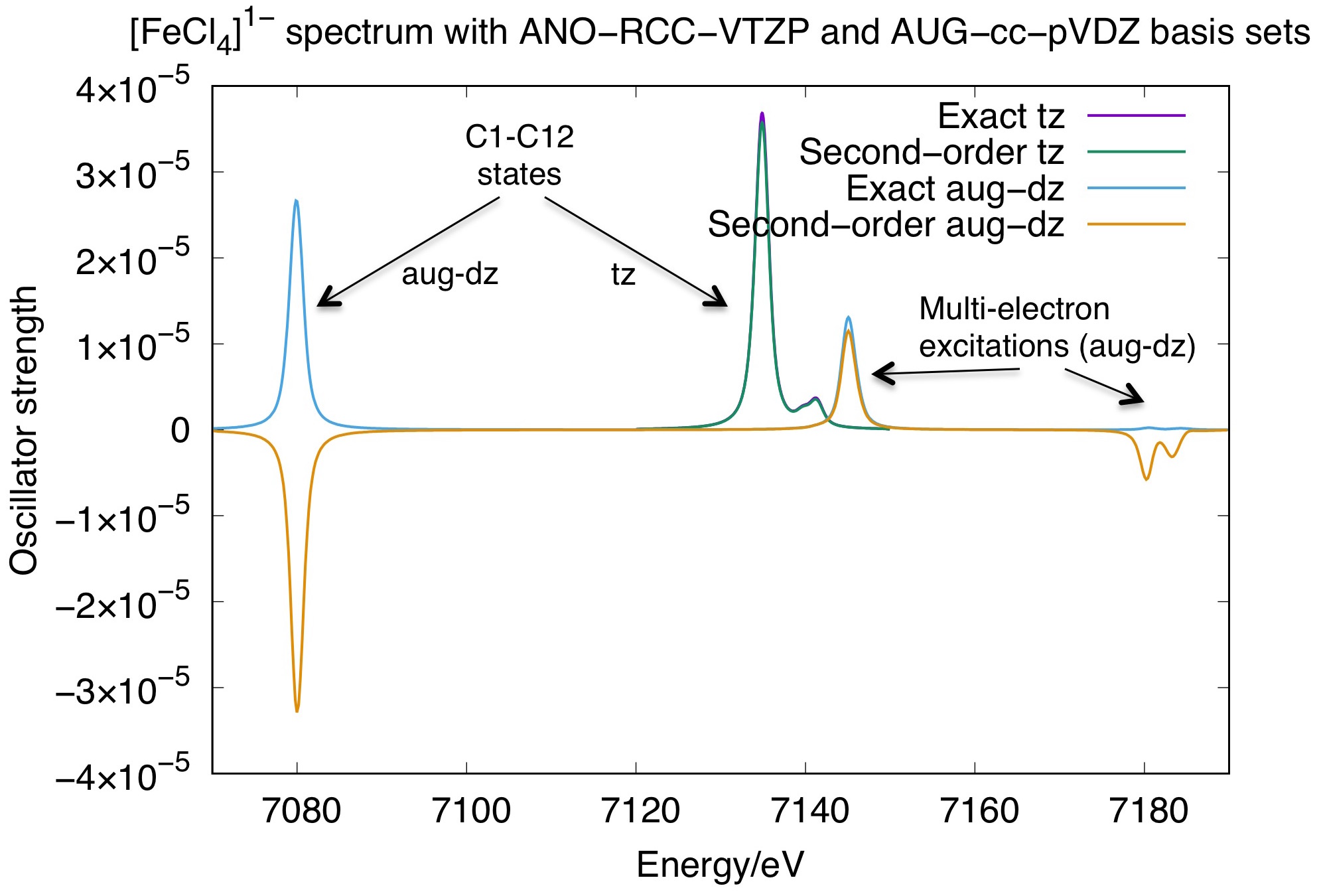
Figure 3: A comparison of the spectra for $[FeCl_{4}]^{1-}$ using the exact operator and the second-order expansion in the AUG-cc-pVDZ and ANO-RCC-VTZP basis sets. Note that the spectra are energetically shifted due to different descriptions of the core orbitals. The spectra for the second order was previously published in Ref. Sørensen et al. (2017b).

III.4 Origin dependence of metal K pre edge XAS of iron dimer

As shown by Bernadotte et al. , the full second-order expansion is origin independent in the velocity gauge.Lehtola et al. (2012); Bernadotte et al. (2012) We showed that this also holds in the true length gauge, but not in the mixed gauge that is typically referred to as the length gauge.Sørensen et al. (2017b, a) This becomes an issue for an iron dimer that lacks a natural origin for the multipole expansion. As the individual iron sites in the dimer are asymmetric, metal 4p orbitals mix into the valence space, giving dipole-allowed transitions in the pre-edge, which leads to instability for the second-order expansion.

In Sørensen et al. (2017b) we showed that if the origin was placed close to the center of mass the change in the spectrum for the so-called origin independent quadrupole oscillator strengths in a mixed gauge was minor while at slightly larger distances significant changes in the spectrum could be observed, see Figure 4. The intensity of the second peak is most sensitive, which is consistent with larger electric-dipole contributions.

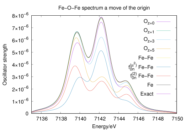
Figure 4: A comparison of the spectra for Fe-O-Fe with the origin in the oxygen atom (O_x=0), origin moved along the $x$-axis (O_x=d), where $d$ is the distance, the origin in the middle between the two Fe atoms (Fe-Fe) and the origin placed on one of the Fe atom (Fe) and the exact operator in the ANO-RCC-VTZP basis set. The $f_{0n}^{(\mu^{2})}$ and $f_{0n}^{(2)}$ contributions are shown with the origin placed between the two Fe atoms. The data from the origin independent quadrupole oscillator strengths in a mixed gauge is taken from Ref. Sørensen et al. (2017b).

From Figure 4 we see that the exact operator and the oscillator strengths in the mixed gauge agree rather well, both with respect to the shape and the total intensity of the spectrum. Previous K pre-edge calculations using the mixed gauge are therefore most likely of acceptable quality.

IV Perspective

While the results in Sec. III and implementation in Sec. II.2 does show that the exact semi-classical light-matter interaction is easier to implement and numerically better than the multipole expansion for the weak field limit we believe that the real strength of the approach lies in the strong field regime.

IV.1 Real-time dependent light matter interaction

For strong fields, where the perturbative treatment of the light-matter interaction breaks down, the multipole expansion is still used and the light-matter interaction is usually treated in the dipole approximation

$$\hat{H}=\hat{H}_{0}-\bm{E}(t)\bm{\mu}.$$ (33)

If the wave function is expanded in a Gaussian basis then the exact same as evaluation of the exact semi-classical light matter interaction presented in Section II.2 could be used without any significantly added cost to a more general Hamiltonian

$$\hat{H}=\hat{H}_{0}+\hat{U}(t),$$ (34)

where $\hat{U}(t)$ is given by Eq. 2, to significantly improve the description of a laser-pulse interacting with a target. Going beyond the dipole approximation is particularly interesting for X-ray spectroscopy and in general for very short wave lengths where the pulse varies over the size of the molecule, very strong time-dependent magnetic fields, for multi-photon processes where the field becomes strong enough to see contributions from the $(\bm{A}^{2})$ in Eq. 4. While the differences in oscillator strengths seems minor with well-behaving basis sets in the static case, see Figure 4, these differences should quickly become apparent in the dynamic case where it is the interaction with the laser field that drives the dynamics since small initial differences in interaction can quickly grow large. In the real-time dependent description the explicit strength and shape of the field would also have to be included though these are merely the values of a time dependent function describing the envelope and strength of the field.

V Conclusion

We have presented a very easy way to implement the exact semi-classical light-matter interaction from Eq. 2 where the integrals either can be calculated analytically or extending the standard Gauss-Hermite integral evaluation to complex numbers. We show that the integral evaluation is akin to a Fourier transformation from real to $k$-space of the overlap of the basis functions and that the electric, magnetic and quadratic term $(\bm{A}^{2})$ can be evaluated in the same way.

The main advantages of the exact operator is seven-fold: i) it is cheaper to calculate than higher order terms in the multipole expansion, ii) there is never negative oscillator strengths, iii) always origin independent, iv) easy to extend to time-dependent calculations, v) appears to be more numerically stable, and vi) less sensitive to the choice of basis set since the basis set only have to work for a single type of integrand and not a multitude of different integrands as in the multipole expansion Crossley (1969). Additionally, vii) using the exact operator also avoids the faulty interpretation of electric and magnetic terms in the multipole expansion since this interpretation always will depend on the choice of coordinate system since none of these terms are observable. Due to the ease at which the exact semi-classical light matter interaction can be implemented, the numerical, theoretical and interpretation advantages we do not see the need for the multipole expansion anymore for transition moments.

We show numerical examples of the exact operator on [CuCl₄]^2- where the angle between beam and sample is known and on [FeCl₄]^1- and Fe-O-Fe where an isotropic averaging is performed. For the bis(creatinium)tetrachlorocuprate(II) crystal we have showed that with an angular resolved spectrum can discern the symmetry of the [CuCl₄]^2- unit. The numerical stability of the exact operator, even in basis sets performing poorly for the multipole expansion, has been demonstrated for the [FeCl₄]^1- molecule. In the AUG-cc-pVDZ basis set even transitions with negative second order oscillator strengths the exact operator gave results close to those obtained for the exact operator in the better ANO-RCC-VTZP basis set where the second order oscillator strengths was positive. In fact the difference between the oscillator strengths for the exact operator in the ANO-RCC-VTZP and AUG-cc-pVDZ basis sets is about the same as the difference between the exact operator and the second order in the ANO-RCC-VTZP basis set. If the very good numerical performance of the exact operator, seen in these preliminary calculations, is general is currently being investigated. Finally for Fe-O-Fe we reproduce the spectrum previously publishedSørensen et al. (2017b) which together with the results for [FeCl₄]^1- in the ANO-RCC-VTZP basis shows that when good basis sets are used then the multipole expansion does produce results close to that of the exact operator.

While using the exact operator does give a significant improvement over the multipole expansion for weak fields we do believe that the real strength of the approach will be in the dynamics of strong fields. We are therefore currently exploring the options of using the exact operator in time-dependent calculations since this will give more accurate dynamics for molecules in strong laser fields, here in particularly for very short wave lengths, like X-rays, where the field varies over the range of the molecule or an atom, where terms above the dipole becomes important or where the $\boldmath{A}^{2}$ becomes important.

The implementation of the exact operator for electric and magnetic fields along with the integrals the for quadratic term $(\bm{A}^{2})$ are freely available in OpenMolcas.”https://gitlab.com/Molcas/OpenMolcas”

References

- edited by J. Lindon and Koppenaal (2016) G. E. T. edited by J. Lindon and D. Koppenaal, Encyclopedia of Spectroscopy and Spectrometry, 3rd ed. (Academic Press, 2016).
- Abbott et al. (2016) B. P. Abbott, R. Abbott, T. D. Abbott, et al. (LIGO Scientific Collaboration and Virgo Collaboration), Phys. Rev. Lett. 116, 061102 (2016).
- (3) G. W. F. D. (Ed.), Springer Handbooks of Atomic, Molecular, and Optical Physics (Springer, Berlin [et. al], 2006).
- Joachain et al. (2000) C. J. Joachain, M. Dörr, and N. Kylstra, Adv. Mol. Opt. Phys. 42, 225 (2000).
- Posthumus (2004) J. H. Posthumus, Rep. Prog. Phys. 67, 623 (2004).
- Bernadotte et al. (2012) S. Bernadotte, A. J. Atkins, and C. R. Jacob, J. Chem. Phys. 137, 204106 (2012).
- Sørensen et al. (2017a) L. K. Sørensen, R. Lindh, and M. Lundberg, Chem. Phys. Lett. 683, 536 (2017a).
- Sørensen et al. (2017b) L. K. Sørensen, M. Guo, R. Lindh, and M. Lundberg, Mol. Phys. 115, 174 (2017b).
- Crossley (1969) R. J. S. Crossley, Adv. At. Mol. Phys. 5, 237 (1969).
- Lehtola et al. (2012) J. Lehtola, M. Hakala, A. Sakko, and K. Hämäläinen, J. Comp. Chem. 33, 1572 (2012).
- List et al. (2015) N. H. List, J. Kauczor, T. Saue, H. J. Aa. Jensen, and P. Norman, J. Chem. Phys. 142, 244111 (2015).
- List et al. (2017) N. H. List, T. Saue, and P. Norman, Mol. Phys. 115, 63 (2017).
- Shulman et al. (1976) G. Shulman, Y. Yafet, P. Eisenberger, and W. Blumberg, Proceedings of the National Academy of Sciences 73, 1384 (1976).
- Hahn et al. (1982) J. E. Hahn, R. A. Scott, K. O. Hodgson, S. Doniach, S. R. Desjardins, and E. I. Solomon, Chem. Phys. Lett. 88, 595 (1982).
- Westre et al. (1997) T. E. Westre, P. Kennepohl, J. G. DeWitt, B. Hedman, K. O. Hodgson, and E. I. Solomon, J. Am. Chem. Soc. 119, 6297 (1997).
- Olsen et al. (1988) J. Olsen, B. O. Roos, P. Jørgensen, and H. J. Aa. Jensen, J. Chem. Phys. 89, 2185 (1988).
- Malmqvist et al. (1990) P.-Å. Malmqvist, A. Rendell, and B. O. Roos, J. Phys. Chem. 94, 5477 (1990).
- Josefsson et al. (2012) I. Josefsson, K. Kunnus, S. Schreck, A. Föhlisch, F. de Groot, P. Wernet, and M. Odelius, J. Phys. Chem. Lett 3, 3565 (2012).
- Bokarev et al. (2013) S. I. Bokarev, M. Dantz, E. Suljoti, O. Kühn, and E. F. Aziz, Phys. Rev. Lett 111, 083002 (2013).
- Pinjari et al. (2014) R. V. Pinjari, M. G. Delcey, M. Guo, M. Odelius, and M. Lundberg, J. Chem. Phys 141, 124116 (2014).
- Guo et al. (2016a) M. Guo, L. K. Sørensen, M. G. Delcey, R. V. Pinjari, and M. Lundberg, Phys. Chem. Chem. Phys. 18, 3250 (2016a).
- Guo et al. (2016b) M. Guo, E. Källman, L. K. Sørensen, M. G. Delcey, R. V. Pinjari, and M. Lundberg, J. Phys. Chem. A 120, 5848 (2016b).
- Gubarev et al. (2001) F. V. Gubarev, L. Stodolsky, and V. I. Zakharov, Chem. Phys. Lett. 86, 2220 (2001).
- J. Lestrange et al. (2015) P. J. Lestrange, F. Egidi, and X. Li, J. Chem. Phys. 143, 234103 (2015).
- Polášek and Čarsky (2002) M. Polášek and P. Čarsky, J. Comput. Phys. 181, 1 (2002).
- Čarsky and Polášek (1998) P. Čarsky and M. Polášek, J. Comput. Phys. 143, 266 (1998).
- Füsti-Molnar and Pulay (2002) L. Füsti-Molnar and P. Pulay, J. Chem. Phys. 116, 7795 (2002).
- Devaney and Wolf (1974) A. J. Devaney and E. Wolf, J. Math. Phys. 15, 234 (1974).
- Malmqvist (1986) P. Å. Malmqvist, Int. J. Quantum Chem. 30, 479 (1986).
- (30) ”https://gitlab.com/Molcas/OpenMolcas”, .
- Malmqvist et al. (2002) P. Å. Malmqvist, B. O. Roos, and B. Schimmelpfennig, Chem. Phys. Lett. 357, 230 (2002).
- Barron (2004) L. D. Barron, Molecular Light Scattering and Optical Activity, 2nd ed. (Cambridge University Press, Cambridge, 2004).
- Lebedev (1975) V. I. Lebedev, USSR Comput. Math. Math. Phys. 15, 44 (1975).
- Lebedev (1976) V. I. Lebedev, USSR Comput. Math. Math. Phys. 16, 10 (1976).
- Lebedev (1977) V. I. Lebedev, Sib. Math. J. 18, 99 (1977).
- Lebedevand and Skorokhodov (1992) V. I. Lebedevand and A. Skorokhodov, Russ. Acad. Sci. Dokl. Math. 45, 587 (1992).
- Lebedev (1995) V. I. Lebedev, Russ. Acad. Sci. Dokl. Math. 50, 283 (1995).
- Lebedevand and Laikov (1999) V. I. Lebedevand and D. N. Laikov, Dokl. Math. 59, 477 (1999).
- Warnke et al. (2010) Z. Warnke, E. Stycze, D. Wyrzykowski, A. Sikorski, J. Klak, and J. Mroziski., Struct Chem 21, 285 (2010).
- Douglas and Kroll (1974) M. Douglas and N. M. Kroll, Ann. Phys. 82, 89 (1974).
- Heß (1986) B. A. Heß, Phys. Rev. A 33, 3742 (1986).
- Roos et al. (2005) B. O. Roos, R. Lindh, P.-Å. Malmqvist, V. Veryazov, and P.-O. Widmark, J. Chem. Phys. 109, 6575 (2005).
- Roos et al. (2004) B. O. Roos, R. Lindh, P.-Å. Malmqvist, V. Veryazov, and P.-O. Widmark, J. Phys. Chem. A 108, 2851 (2004).
- Malmqvist and Roos (1989) P.-Å. Malmqvist and B. O. Roos, Chem. Phys. Lett. 155, 189 (1989).