Proximal-Free ADMM for Decentralized Composite Optimization via Graph Simplification

Abstract

We consider the problem of decentralized composite optimization over a symmetric connected graph, in which each node holds its own agent-specific private convex functions, and communications are only allowed between nodes with direct links. A variety of algorithms have been proposed to solve such a problem in an alternating direction method of multiplier (ADMM) framework. Many of these algorithms, however, need to include some proximal term in the augmented Lagrangian function such that the resulting algorithm can be implemented in a decentralized manner. The use of the proximal term slows down the convergence speed because it forces the current solution to stay close to the solution obtained in the previous iteration. To address this issue, in this paper, we first introduce the notion of simplest bipartite graph, which is defined as a bipartite graph that has a minimum number of edges to keep the graph connected. A simple two-step message passing-based procedure is proposed to find a simplest bipartite graph associated with the original graph. We show that the simplest bipartite graph has some interesting properties. By utilizing these properties, an ADMM without involving any proximal terms can be developed to perform decentralized composite optimization over the simplest bipartite graph. Simulation results show that our proposed method achieves a much faster convergence speed than existing state-of-the-art decentralized algorithms.

I Introduction

A network with multiple agents is called a multi-agent network, which can be described by a graph. In a multi-agent network, each agent is equipped with sensing, communication and computing abilities, such that the agents are able to collaboratively accomplish computational tasks [1]. Among the various tasks that a multi-agent system can undertake, distributed optimization is of significant importance. There are basically two different approaches for distributed optimization, i.e. centralized and decentralized approaches. A centralized approach works in a center-local (master-worker) fashion [2], namely, local agents (workers) are only connected with the center agent (master). In each iteration, each local agent sends their local data to the center agent, and the center agent sends the processed data back to each local agent. This operation mode brings a heavy burden on the center agent because the center agent needs to communicate with all local agents. Another approach is the so called decentralized methods which has attracted much attention over the past few years. For decentralized methods, a center agent is no longer needed. Each agent has only access to the information of its neighboring nodes, namely, communications are only allowed among neighboring nodes. Such a decentralized operation involves a very low communication cost for each agent. In addition, decentralized methods are robust to communication disruption, node failure or malfunctioning. Due to these attractive merits, decentralized methods have found applications in various fields, including information processing over sensor networks [3], aircraft or vehicle networks [4], cooperative spectrum sensing in cognitive radios [5], monitoring and optimization of smart grids [6], distributed control of networked robots [7], distributed machine learning [8, 9] and wireless communications [10].

The research on decentralized optimization originates from 1980s [11, 12], the time when large-scale networks emerged. Many earlier methods, such as the incremental subgradient methods [13, 14] and the incremental proximal methods [15], are only applicable to a special ring type network, which is restrictive in real applications. The recently proposed method [16] also follows this line. To accommodate general networks, a distributed subgradient method [17] and its variants [18, 19] were proposed. Though simple and easy to implement, these algorithms are very slow due to the use of a diminishing step size.

Many efforts have been made to develop decentralized algorithms with fixed step sizes. Generally, these studies can be divided into second-order methods [20, 21, 22] and first-order methods [23, 24, 25, 26, 27, 28, 29, 30]. Although the second-order methods have a fast convergence rate, they usually incur a high computational complexity since they need to compute the inverse of the Hessian matrix of the objective function. Besides, second-order methods require the objective function to be twice differentiable, which may not be satisfied for many optimization problems. Compared with second-order methods, first-order methods are often considered more preferable due to their simplicity and low computational complexity. Specifically, since consensus among local variables can be formulated as a linear constraint, decentralized first-order methods can be naturally developed in an ADMM or an augmented Lagrangian multiplier (ALM) framework. In [23], decentralized ADMM algorithms were proposed for solving the sparse LASSO problem, in which a node-wise consensus formulation that enforces consensus for each pair of nodes with direct links is used. Based on a same consensus formulation, the work [24] addressed a general single-objective optimization problem, and the works [25, 26] considered decentralized composite optimization problems with a smooth+nonsmooth structure placed on the objective functions. In some other works, e.g. [27, 28, 29, 30], a different consensus formation was employed by resorting to the Laplacian matrix of the underlying graph. To enable decentralized implementation, in these works [27, 28, 29, 30], an extra proximal term expressed as

$$\|\boldsymbol{x}-\boldsymbol{x}(k)\|_{\boldsymbol{W}}^{2}=(\boldsymbol{x}-\boldsymbol{x}(k))^{T}\boldsymbol{W}(\boldsymbol{x}-\boldsymbol{x}(k))$$ (1)

has to be included in the augmented Lagrangian function to eliminate the nonseparable term that demands centralized processing. Here $\boldsymbol{x}$ denotes the optimization variable, $\boldsymbol{x}(k)$ represents the solution obtained in the previous iteration, and $\boldsymbol{W}$ is a carefully chosen positive semi-definite matrix. Although facilitating decentralized implementation, this proximal term has the disadvantage of slowing down the convergence speed because it forces the current solution to stay close to the solution obtained in the previous iteration.

To further improve the convergence speed of the decentralized ADMM, in this paper, we propose a proximal-free ADMM for decentralized composite optimization problems by converting the underlying graph into a simplest bipartite graph. Here the simplest bipartite graph is defined as a bipartite graph that has a minimum number of edges to keep the graph connected. A simple two-step message passing-based procedure is developed to find a simplest bipartite graph associated with the original graph. By utilizing the properties of the simplest bipartite graph, an ADMM without involving any extra proximal terms can be developed. The proposed algorithm exhibits a faster convergence speed than existing state-of-the-art decentralized algorithms. Also, since our proposed method operates over a simplest bipartite graph with a minimum number of edges, the amount of data to be exchanged (among nodes) is considerably reduced compared with other methods. Such a merit makes our proposed algorithm particularly suitable for networks subject to stringent power and communication constraints.

The rest of this paper is organized as follows. We first introduce the basic assumptions and the decentralized composite optimization problem in Section II. We then develop a proximal-free ADMM for single-objective optimization problems in Section III. In Section IV, a simple two-step message passing procedure is proposed to find a simplest bipartite graph associated with the original graph. In Section V, we extend our proposed method to decentralized composite optimization problems. Simulations results are provided in Section VI, followed by concluding remarks in Section VII.

II Problem Formulation

Consider a bidirectionally connected network consisting of $l$ nodes and $m$ edges. The network is described by a symmetric directed graph $G=\left\{{V,E}\right\}$, where $V$ is the set of nodes and $E$ is the set of edges. At each iteration, every node communicates with its neighboring nodes. The communication is assumed to be synchronized. In this paper, we consider a decentralized composite optimization problem expressed as

$$\mathop{\min}\limits_{\boldsymbol{x}}\sum\limits_{i=1}^{l}{{f_{i}}\left(\boldsymbol{x}\right)+{g_{i}}\left(\boldsymbol{x}\right)}$$ (2)

where $\boldsymbol{x}\in{\mathbb{R}^{n}}$ is the optimization variable shared by all the objective functions, ${f_{i}},{g_{i}}:\mathbb{R}^{n}\rightarrow\mathbb{R}\cup\{\infty\}$ are proper, lower semicontinuous convex functions (possibly nondifferentiable), only known to the $i$th agent. We have the following assumption regarding the functions ${f_{i}}$ and ${g_{i}}$.

Assumption 1

The proximal mapping of $g_{i},\forall i$, defined as

$$\text{prox}_{g_{i}}(\boldsymbol{y})\triangleq\arg\min_{\boldsymbol{x}}g_{i}(\boldsymbol{x})+\frac{1}{2}\|\boldsymbol{x}-\boldsymbol{y}\|_{2}^{2}$$ (3)

has a closed-form solution. For $f_{i},\forall i$, either its proximal mapping has a closed-form solution or it is a smooth convex function with Lipschitz continuous gradient, i.e.

$${\left\|{\nabla{f_{i}}\left(\boldsymbol{x}\right)-\nabla{f_{i}}\left(\boldsymbol{y}\right)}\right\|_{2}}\leq{L_{f}}{\left\|{\boldsymbol{x}-\boldsymbol{y}}\right\|_{2}},\quad\forall\boldsymbol{x},\boldsymbol{y}$$ (4)

where $L_{f}$ is the Lipschitz constant. To avoid triviality, it is assumed that the proximal mapping of $f_{i}+g_{i}$ does not have a closed-form solution.

Assume each agent $i$ holds a local copy ${\boldsymbol{x}_{i}}\in\mathbb{R}^{n}$ of the global variable $\boldsymbol{x}$ in problem (2). Define

$$f({\tilde{\boldsymbol{x}}})\triangleq\sum\limits_{i=1}^{l}{{f_{i}}\left({{\boldsymbol{x}_{i}}}\right)}\quad g({\tilde{\boldsymbol{x}}})\triangleq\sum\limits_{i=1}^{l}{{g_{i}}\left({{\boldsymbol{x}_{i}}}\right)}$$ (5)

where $\tilde{\boldsymbol{x}}\buildrel\Delta\over{=}\left[\boldsymbol{x}_{1}^{T}\phantom{0}\boldsymbol{x}_{2}^{T}\phantom{0}\ldots\phantom{0}\boldsymbol{x}_{l}^{T}\right]^{T}\in\mathbb{R}^{nl}$ is a stacked column vector. We say that $\tilde{\boldsymbol{x}}$ is consensual if ${\boldsymbol{x}_{1}}={\boldsymbol{x}_{2}}=\ldots={\boldsymbol{x}_{l}}$. Thus problem (2) can be reformulated as

$$\min_{\tilde{\boldsymbol{x}}} \quad f({\tilde{\boldsymbol{x}}})+g({\tilde{\boldsymbol{x}}})$$

s.t. $$\quad\tilde{\boldsymbol{L}}\tilde{\boldsymbol{x}}=\boldsymbol{0}$$ (6)

where $\tilde{\boldsymbol{L}}\triangleq\boldsymbol{L}\otimes{\boldsymbol{I}_{n}}$, $\otimes$ denotes the Kronecker product, ${\boldsymbol{I}_{n}}\in\mathbb{R}^{n\times n}$ is an identity matrix, $\boldsymbol{L}\in\mathbb{R}^{l\times l}$ is the Laplacian matrix of the graph $G$ defined as

$$L_{i,j}=\left\{\begin{array}[]{l}\deg(V_{i}),\text{if $i=j$}\\ -1,\text{$i\neq j$, node $i$ and $j$ are connected}\\ 0,\text{otherwise}\end{array}\right.$$ (10)

in which $\deg(V_{i})$ is the degree of the $i$th node. Since $\text{null}(\boldsymbol{L})=\text{span}\{\boldsymbol{1}\}$, we know that the variable ${\tilde{\boldsymbol{x}}}$ is consensual if the constraint in problem (6) is satisfied.

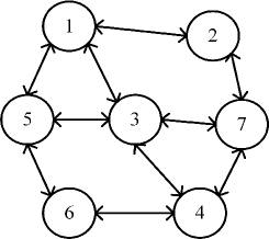
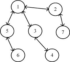
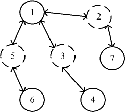
Figure 1: Left: The original graph; Middle: The corresponding minimum spanning tree; Right: The simplest bipartite graph (nodes belonging to the set $H$ are plotted with solid line, while those in the set $T$ are plotted with dashed line)

III Proximal-Free ADMM: Single-Objective Optimization

To more clearly explain the idea of our proposed algorithm, we start by discussing a single-objective optimization problem, which is a special case of the composite optimization problem. The single-objective problem is formulated as

$$\min_{\tilde{\boldsymbol{x}}} \quad f(\tilde{\boldsymbol{x}})$$

s.t. $$\quad\tilde{\boldsymbol{L}}\tilde{\boldsymbol{x}}=\boldsymbol{0}$$ (11)

Before proceeding, we first introduce the notion of simplest bipartite graph. Here the simplest bipartite graph is defined as a bipartite graph that has a minimum number of edges keeping the graph connected (see Fig. 1). More precisely, given a graph $G=\{V,E\}$, a simplest bipartite graph can be denoted as $G_{sbi}=\{H,T,E_{0}\}$, in which $E_{0}\in E$ is chosen such that $\{V,E_{0}\}$ is a minimum spanning tree (MTS) for $G$, and $H$ and $T$ are two disjoint sets ($H\cap T=\varnothing$ and $V=H\cup T$) such that each edge in $E_{0}$ connects a pair of nodes not belonging to the same set. Specifically, the simplest bipartite graph has the same $l$ nodes as in $G=\{{V,E}\}$, yet only keeps $l-1$ edges. As will be shown later, the simplest bipartite graph can be readily obtained from an MST of the graph $G$.

Given a graph $G$, suppose its simplest bipartite graph $G_{sbi}=\{H,T,E_{0}\}$ is now available to us. Let $\boldsymbol{L}_{G_{sbi}}$ denote the Laplacian matrix associated with the simplest bipartite graph. Since $G_{sbi}$ is still a connected graph, $\tilde{\boldsymbol{L}}$ in (III) can be replaced with $\boldsymbol{\tilde{L}}_{G_{sbi}}\triangleq\boldsymbol{L}_{G_{sbi}}\otimes{\boldsymbol{I}_{n}}$, which yields

$$\min_{\tilde{\boldsymbol{x}}} \quad\sum\limits_{i\in H}f_{i}(\boldsymbol{x}_{i})+\sum\limits_{i\in T}f_{i}(\boldsymbol{x}_{i})$$

s.t. $$\quad\tilde{\boldsymbol{L}}_{G_{sbi}}\tilde{\boldsymbol{x}}=\boldsymbol{0}$$ (12)

In the following, we will explore some important properties about $\boldsymbol{\tilde{L}}_{G_{sbi}}$. As will be shown, these properties play a crucial role in developing a proximal-free decentralized algorithm.

Lemma 1 ([31])

Given an undirected graph $G=\{V,E\}$ consisting of $l$ nodes and $m$ edges, its corresponding Laplacian matrix $\boldsymbol{L}$ defined in (10) can be decomposed as

$$\boldsymbol{L}=\boldsymbol{X}^{T}\boldsymbol{X}$$ (13)

where $\boldsymbol{X}\in\mathbb{R}^{m\times l}$ is the oriented incidence matrix of the undirected graph $G$. The oriented incidence matrix is the incidence matrix of any orientation of the graph, with its rows and columns indexed by the edges and vertices of $G$, respectively. Specifically, for an edge connecting two vertices $i$ and $j$, the row of $\boldsymbol{X}$ used to describe this edge has two nonzero elements, with its $i$th entry and $j$th entry equal to $1$ and $-1$ (or $-1$ and $1$) respectively. We have the following property regarding $\boldsymbol{X}$:

• If two nodes, say node $i$ and $j$, in $G$ are unconnected, then $\boldsymbol{X}_{i}^{T}\boldsymbol{X}_{j}=0$, where $\boldsymbol{X}_{i}$ and $\boldsymbol{X}_{j}$ denote the $i$th and $j$th columns of $\boldsymbol{X}$ respectively. While if node $i$ and $j$ are connected, then $\boldsymbol{X}_{i}^{T}\boldsymbol{X}_{j}=-1$. Moreover, $\boldsymbol{X}_{i}^{T}\boldsymbol{X}_{i}=\text{deg}(V_{i})$, where $\text{deg}(V_{i})$ is the degree of the $i$th node.

Proof:

See [31]. ∎

Besides, we have the following important property regarding the incidence matrix associated with a simplest bipartite graph.

Lemma 2

Given a simplest bipartite graph $G_{sbi}=\{V(H,T),E_{0}\}$, the oriented incidence matrix $\boldsymbol{X}\in\mathbb{R}^{(l-1)\times l}$ associated with $G_{sbi}$ is a full row rank matrix.

Proof:

See Appendix A. ∎

Let $\boldsymbol{A}$ denote the incidence matrix of the simplest bipartite graph $G_{sbi}=\{V(H,T),E_{0}\}$. From Lemma 1, we have $\boldsymbol{L}_{G_{sbi}}=\boldsymbol{A}^{T}\boldsymbol{A}$ and ${\tilde{\boldsymbol{L}}}_{G_{sbi}}=(\boldsymbol{A}\otimes\boldsymbol{I}_{n}))^{T}(\boldsymbol{A}\otimes\boldsymbol{I}_{n})$. According to Lemma 2, the incidence matrix $\boldsymbol{A}$ is full row rank. Therefore problem (III) can be equivalently written as

$$\min_{\tilde{\boldsymbol{x}}} \quad\sum\limits_{i\in H}f_{i}(\boldsymbol{x}_{i})+\sum\limits_{i\in T}f_{i}(\boldsymbol{x}_{i})$$

s.t. $$\quad(\boldsymbol{A}\otimes\boldsymbol{I}_{n})\tilde{\boldsymbol{x}}=\boldsymbol{0}$$ (14)

We divide all the columns of $\boldsymbol{A}$ into two groups, i.e. $\boldsymbol{A}_{H}$ and $\boldsymbol{A}_{T}$, in which the indexes of the columns in $\boldsymbol{A}_{H}$ ($\boldsymbol{A}_{T}$) are specified by the set $H$ ($T$). Similarly, let $\tilde{\boldsymbol{x}}_{H}$ ($\tilde{\boldsymbol{x}}_{T}$) denote a stacked column vector consisting of the local variables hold by the nodes whose indexes belong to the set $H$ ($T$). Thus the optimization (III) can be rewritten as

$$\min_{\tilde{\boldsymbol{x}}} \quad\sum\limits_{i\in H}f_{i}(\boldsymbol{x}_{i})+\sum\limits_{i\in T}f_{i}(\boldsymbol{x}_{i})$$

s.t. $$\quad(\boldsymbol{A}_{H}\otimes\boldsymbol{I}_{n})\tilde{\boldsymbol{x}}_{H}+(\boldsymbol{A}_{T}\otimes\boldsymbol{I}_{n})\tilde{\boldsymbol{x}}_{T}=\boldsymbol{0}$$ (15)

Also, to facilitate our subsequent exposition, we assume the dimension of the local variable, $n$, is equal to $1$. In such a case, the problem (III) is simplified as

$$\min_{\tilde{\boldsymbol{x}}} \quad\sum\limits_{i\in H}f_{i}(\boldsymbol{x}_{i})+\sum\limits_{i\in T}f_{i}(\boldsymbol{x}_{i})$$

s.t. $$\quad\boldsymbol{A}_{H}\tilde{\boldsymbol{x}}_{H}+\boldsymbol{A}_{T}\tilde{\boldsymbol{x}}_{T}=\boldsymbol{0}$$ (16)

Note that the following derivations can be readily extended to the scenario where $n>1$. Also, it is noted that the formulation of (III)–(III) involves an explicit expression of $\boldsymbol{A}$. Nevertheless, as will be shown later, our developed algorithm only requires the knowledge of $\boldsymbol{L}_{G_{sbi}}=\boldsymbol{A}^{T}\boldsymbol{A}$, which is readily available to us.

Since the optimization (III) is a typical two-block problem, the well-established ADMM can be used to solve this problem, which yields the following three sub-problems:

$${{\tilde{\boldsymbol{x}}}_{H}}(k+1)= \arg\min_{{\tilde{\boldsymbol{x}}}_{H}}\sum_{i\in H}f_{i}({\boldsymbol{x}}_{i})+$$

$$\frac{\sigma}{2}\|{{\boldsymbol{A}}_{H}}{{\tilde{\boldsymbol{x}}}_{H}}+{{\boldsymbol{A}}_{T}}{{\tilde{\boldsymbol{x}}}_{T}}(k)+\frac{1}{\sigma}\boldsymbol{\lambda}(k)\|_{2}^{2}$$

$${\tilde{\boldsymbol{x}}_{T}}(k+1)= \arg\min_{{\tilde{\boldsymbol{x}}}_{T}}\sum_{i\in T}f_{i}({\boldsymbol{x}}_{i})$$

$$+\frac{\sigma}{2}\|{{\boldsymbol{A}}_{H}}{{\tilde{\boldsymbol{x}}}_{H}}(k+1)+{{\boldsymbol{A}}_{T}}{{\tilde{\boldsymbol{x}}}_{T}}+\frac{1}{\sigma}\boldsymbol{\lambda}(k)\|_{2}^{2}$$

$$\boldsymbol{\lambda}(k+1)= \boldsymbol{\lambda}(k)+\sigma({{\boldsymbol{A}}_{H}}{{\tilde{\boldsymbol{x}}}_{H}}(k+1)+{{\boldsymbol{A}}_{T}}{\tilde{{\boldsymbol{x}}}_{T}}(k+1))$$ (17)

where $\sigma$ is a parameter of user’s choice. We will show that the proposed algorithm, without resorting to proximal terms, can be solved in a decentralized manner.

Let us first examine the $\boldsymbol{\lambda}$-subproblem. According to the update formula of $\boldsymbol{\lambda}(k+1)$, we have

$$\boldsymbol{\lambda}(k+1) =\boldsymbol{\lambda}(k)+\sigma({{\boldsymbol{A}}_{H}}{{\tilde{\boldsymbol{x}}}_{H}}(k+1)+{{\boldsymbol{A}}_{T}}{{\tilde{\boldsymbol{x}}}_{T}}(k+1))$$

$$=\boldsymbol{\lambda}(0)+\sum\limits_{j=0}^{k}\sigma({{\boldsymbol{A}}_{H}}{{\tilde{\boldsymbol{x}}}_{H}}(j+1)+{{\boldsymbol{A}}_{T}}{{\tilde{\boldsymbol{x}}}_{T}}(j+1))$$ (18)

Since $\boldsymbol{\lambda}(0)$ can be an arbitrarily initial vector, we simply set it to be $\boldsymbol{\lambda}(0)=\boldsymbol{0}$. In our proposed algorithm, the $\boldsymbol{\lambda}$-update can be merged into the update of ${\tilde{\boldsymbol{x}}_{H}}(k+1)$ and ${\tilde{\boldsymbol{x}}_{T}}(k+1)$. Take the ${\tilde{\boldsymbol{x}}_{H}}$-subproblem as an example. Substituting (III) into the ${\tilde{\boldsymbol{x}}_{H}}$-subproblem yields

$${\tilde{\boldsymbol{x}}_{H}}(k+1)= \arg\mathop{\min}\limits_{{\tilde{\boldsymbol{x}}}_{H}}\sum_{i\in H}f_{i}({\boldsymbol{x}}_{i})+\frac{\sigma}{2}\|{{\boldsymbol{A}}_{H}}{{\tilde{\boldsymbol{x}}}_{H}}+{{\boldsymbol{A}}_{T}}{{\tilde{\boldsymbol{x}}}_{T}}(k)$$

$$+\sum\limits_{j=0}^{k-1}({{\boldsymbol{A}_{H}}}\tilde{{{\boldsymbol{x}}}}_{H}(j+1)+{{\boldsymbol{A}}_{T}}{{\tilde{\boldsymbol{x}}}_{T}}(j+1))\|_{2}^{2}$$ (19)

Recalling Lemma 1, we know that $\boldsymbol{D}_{H}\triangleq\boldsymbol{A}_{H}^{T}\boldsymbol{A}_{H}$ and $\boldsymbol{D}_{T}\triangleq\boldsymbol{A}_{T}^{T}\boldsymbol{A}_{T}$ are diagonal matrices with its diagonal elements equal to the degrees of the corresponding nodes. Based on this result, (III) can be rewritten as

$${\tilde{\boldsymbol{x}}}_{H}(k+1)= \arg\mathop{\min}\limits_{\tilde{\boldsymbol{x}}_{H}}\sum_{i\in H}f_{i}(\boldsymbol{x}_{i})+\frac{\sigma}{2}\|{\boldsymbol{D}}_{H}^{\frac{1}{2}}{\tilde{\boldsymbol{x}}}_{H}+\tilde{\boldsymbol{d}}_{H}\|_{2}^{2}$$ (20)

where

$$\tilde{\boldsymbol{d}}_{H}\triangleq[\boldsymbol{d}_{i_{1}}^{T}\phantom{0}\ldots\phantom{0}\boldsymbol{d}_{i_{|H|}}^{T}]^{T}\quad i_{1},\ldots,i_{|H|}\in H$$

$$\boldsymbol{d}_{i}\triangleq\mu_{i}^{\frac{1}{2}}\sum\limits_{j=0}^{k-1}{\boldsymbol{x}_{i}}(j+1)+\mu_{i}^{-\frac{1}{2}}\boldsymbol{A}_{i}^{T}{\boldsymbol{A}_{T}}\bigg{(}{\tilde{\boldsymbol{x}}_{T}}(k)+\sum\limits_{j=0}^{k-1}{\tilde{\boldsymbol{x}}_{T}}(j+1)\bigg{)}$$ (21)

in which $\mu_{i}\triangleq\text{deg}(V_{i})$ is the degree of the $i$th node. Since ${\boldsymbol{D}}_{H}$ in (20) is a diagonal matrix, the problem (20) can be decomposed into a number of independent tasks:

$${\boldsymbol{x}}_{i}(k+1)=\arg\mathop{\min}\limits_{\boldsymbol{x}_{i}}f_{i}(\boldsymbol{x}_{i})+\frac{\sigma}{2}\|\mu_{i}^{\frac{1}{2}}\boldsymbol{x}_{i}+\boldsymbol{d}_{i}\|_{2}^{2},\ i\in H$$ (22)

Clearly, ${\boldsymbol{x}}_{i}(k+1)$ is the solution of the proximal mapping of $f_{i}$. If the proximal mapping of $f_{i}$ has a closed-form solution, then ${\boldsymbol{x}}_{i}(k+1)$ can be easily obtained. On the other hand, if the proximal mapping of $f_{i}$ dose not have a closed-form solution, but $f_{i}$ is continuously differentiable and has Lipschitz continuous gradient, then we can replace $f_{i}(\boldsymbol{x}_{i})$ with its upper bound [32]:

$$f_{i}(\boldsymbol{x}_{i}(k))+\langle\boldsymbol{x}_{i}-\boldsymbol{x}_{i}(k),\nabla f_{i}(\boldsymbol{x}_{i})\rangle+\frac{L_{f_{i}}}{2}\|\boldsymbol{x}_{i}-\boldsymbol{x}_{i}(k)\|_{2}^{2}$$

where $\boldsymbol{x}_{i}(k)$ is the solution obtained in the previous iteration. The resulting problem can thus be easily solved. We see that for node $i$, solving (22) requires the knowledge of $\boldsymbol{d}_{i}$. Nevertheless, the calculation of $\boldsymbol{d}_{i}$ only involves the $i$th node local information and information from its neighboring (i.e. connected) nodes. To see this, recalling Lemma 1, we have $\boldsymbol{A}_{i}^{T}\boldsymbol{A}_{j}=0$ if node $i$ and $j$ are unconnected, while $\boldsymbol{A}_{i}^{T}\boldsymbol{A}_{j}=-1$ if node $i$ and $j$ are connected. Thus the calculation of the following term in $\boldsymbol{d}_{i}$:

$$\boldsymbol{A}_{i}^{T}{\boldsymbol{A}_{T}}({\tilde{\boldsymbol{x}}_{T}}(k)+\sum\limits_{j=0}^{k-1}{\tilde{\boldsymbol{x}}_{T}}(j+1))\quad\forall i\in H$$

only requires information of the nodes that are connected with the $i$th node. Therefore the update of ${\tilde{\boldsymbol{x}}_{H}}(k+1)$ can be readily conducted in a decentralized manner.

Similarly, the ${\tilde{\boldsymbol{x}}_{T}}(k+1)$-subproblem can also be decomposed into a set of tasks, with each task independently solved by each node:

$${\boldsymbol{x}}_{i}(k+1)=\arg\mathop{\min}\limits_{\boldsymbol{x}_{i}}f_{i}(\boldsymbol{x}_{i})+\frac{\sigma}{2}\|\mu_{i}^{\frac{1}{2}}\boldsymbol{x}_{i}+\boldsymbol{d}_{i}\|_{2}^{2},\ i\in T$$ (23)

where

$$\boldsymbol{d}_{i}\triangleq \mu_{i}^{\frac{1}{2}}\sum\limits_{j=0}^{k-1}{\boldsymbol{x}_{i}}(j+1)$$

$$+\mu_{i}^{-\frac{1}{2}}\boldsymbol{A}_{i}^{T}{\boldsymbol{A}_{H}}\bigg{(}{\tilde{\boldsymbol{x}}_{H}}(k+1)+\sum\limits_{j=0}^{k-1}{\tilde{\boldsymbol{x}}_{H}}(j+1)\bigg{)},\ i\in T$$ (24)

It can be easily verified that the update of ${\tilde{\boldsymbol{x}}_{T}}(k+1)$ also admits a decentralized implementation. Based on the above discussion, we see that by utilizing the properties of the simplest bipartite graph, a proximal-free decentralized algorithm can be developed to perform decentralized composite optimization over the simplest bipartite graph. For clarity, the proposed algorithm is summarized in Algorithm 1.

Algorithm 1 Proximal-Free ADMM for solving single-objective optimization problems

  Inputs: $G_{sbi}=\{H,T,E_{0}\}$ , index sets $T$ and $H$, $\sigma$. All the initial vectors are set as $\boldsymbol{0}$.

  while not converge do

  for $i\in H$, parallelly do:

$${\boldsymbol{x}}_{i}(k+1)=\arg\mathop{\min}\limits_{\boldsymbol{x}_{i}}f_{i}(\boldsymbol{x}_{i})+\frac{\sigma}{2}\|\mu_{i}^{\frac{1}{2}}\boldsymbol{x}_{i}+\boldsymbol{d}_{i}\|_{2}^{2},\ i\in H$$

  end forInformation exchange: Let node $i$, $i\in H$, send $\boldsymbol{x}_{i}(k+1)$ to its neighboring nodes.

  for $i\in T$, parallelly do:

$${\boldsymbol{x}}_{i}(k+1)=\arg\mathop{\min}\limits_{\boldsymbol{x}_{i}}f_{i}(\boldsymbol{x}_{i})+\frac{\sigma}{2}\|\mu_{i}^{\frac{1}{2}}\boldsymbol{x}_{i}+\boldsymbol{d}_{i}\|_{2}^{2},\ i\in T$$

  end forInformation exchange: Let node $i$, $i\in T$, send $\boldsymbol{x}_{i}(k+1)$ to its neighboring nodes. end while; Output: $\tilde{\boldsymbol{x}}$;

IV Finding A Simplest Bipartite Graph

A prerequisite of our proposed proximal-free decentralized algorithm is to obtain a simplest bipartite graph corresponding to the original graph. This task can be accomplished via a two-step procedure. First, we search for an MST $G_{ms}=\{V,E_{0}\}$ for the original graph $G=\{V,E\}$. Then, we divide the nodes $V$ into two disjoint sets $H$ and $T$ to form a bipartite graph $G_{bi}=\{H,T,E_{0}\}$. Such a bipartite graph is a simplest bipartite graph because it has a minimum number of edges to keep the graph connected. We will show that both steps can be easily performed without involving complex procedures. It should be noted that a simplest bipartite graph not only facilitates the development of a proximal-free decentralized algorithm, but it also helps substantially reduce the amount of data for transmission within the network because a simplest bipartite graph has a minimum number of edges to keep a graph connected.

IV-A Finding an MST

The problem of finding an MST of a weighted, connected graph has been extensively studied. Many sophisticated methods have been developed to accomplish this task, including the classic Prime algorithm [33] and the Kruskal algorithm [34]. Some of these methods can be directly applied to our problem. Nevertheless, we choose to develop a new algorithm for finding an MST because existing methods are very complicated as they were designed specifically for weighted graphs.

Given a graph $G=\{V,E\}$, we develop a simple message passing scheme to construct an MST $G_{ms}=\{V,E_{0}\}$. The details of the proposed scheme are summarized in Algorithm 2. Briefly speaking, assume a random node (say, node $1$) is activated, with all the other nodes in a sleeping mode. This activated node then sends a probing message to its neighboring nodes (i.e. nodes that are connected to node $1$), say node $2$. After receiving this message, node $2$ is activated from sleeping and sends an acknowledgement signal back to node $1$, such that the link between node $1$ and $2$ is established. Node $2$ then sends the probing message to its neighboring nodes (except node $1$). Such a procedure is repeated until all nodes are activated. During the message passing process, if a node (node $i$) has already been activated and it receives additional probing signals from other nodes, a denial signal will be sent back and no links will be established. On the other hand, if a sleeping node receives probing signals from multiple nodes simultaneously, it randomly selects a node to respond and establishes a link between itself and the selected node, and sends a denial signal to the other nodes. Since only a single edge is created every time when a node (except the first node) is activated, the newly generated graph will have $l-1$ edges in total. Also, it is clear that the graph is connected because each node is connected to node $1$ by direct connection or through a multiple hop route, and thus any two nodes are connected through a certain route. Therefore the graph generated by our message passing scheme is an MST for the original graph $G$. For our proposed message passing scheme, each node needs to communicate with their neighboring nodes only once. Also, the scheme does not need global coordination or synchronization, thus suitable for a decentralized implementation.

Algorithm 2 A message passing algorithm for finding an MST

  Inputs: The original graph $G=\{V,E\}$. All nodes are sleeping

  Begin: Randomly choose a node (denoted as node $1$) and activate this node. Then, let node $1$ send a probing message $p$ to its neighboring nodes.

  while not all nodes are activated do 

  for $i$=$1$:$l$;if node $i$ is sleeping and does not receive $p$ from other nodes, do Keep sleeping.else if node $i$ is sleeping and received $p$ from another node (say node $j$), do \small{1}⃝ Activate node $i$; \small{2}⃝ Send an acknowledgement signal back to node $j$, and establish the link between node $i$ and $j$; \small{3}⃝ Let node $i$ send $p$ to its neighbors.else if node $i$ is sleeping and receiving $p$ from multiple nodes, do \small{1}⃝ Activate node $i$; \small{2}⃝ Randomly select a node, say node $j$, to respond and establish the link between node $i$ and $j$; \small{3}⃝ Let node $i$ send $p$ to its neighboring nodes.else node $i$ is already activated, do  If receiving $p$, send a denial signal to other nodes; otherwise do nothing. end if;

  end for;  end while; Output: $G_{ms}=\{V,E_{0}\}$;

IV-B Obtaining A Simplest Bipartite Graph

Given an MST $G_{0}=\{V,E_{0}\}$, we now discuss how to divide the vertices (nodes) $V$ into two disjoint sets $H$ and $T$ such that each edge in $E_{0}$ connects a pair of nodes not belonging to the same set, i.e. $\{H,T,E_{0}\}$ is a simplest bipartite graph. Again, a message passing scheme can be used to achieve this goal. Start from a randomly selected node (denoted as node $1$), and set a label, say $H$, on node $1$, which means that this node belongs to the set $H$. Node $1$ sends its label information $H$ to its neighboring nodes specified by $E_{0}$, say node $2$. After receiving the label information from node $1$, node $2$ sets itself a label $T$ which is different from what is received from node $1$. The label information of node $2$ is then sent to its neighboring nodes (except node $1$). This procedure is repeated until all nodes set their respective labels. Details of the scheme are provided in Algorithm 3. One may wonder whether a node will receive label information from multiple nodes. The answer is negative. In the message passing scheme, a node only receives label information from a single node. This can be easily shown by contradiction. Suppose that node $i$ receives label information from two nodes, say node $j$ and $k$. This means there is an edge between node $i$ and $j$, and also an edge between $i$ and $k$. Consequently, there will be two routes between node $i$ and node $1$, which contradicts the fact that the underlying graph is an MST. Since each node only receives the label information from a single node, this message passing scheme is guaranteed to find two disjoint sets such that nodes in the same set do not have direct links to connect them. Thus a simplest bipartite graph can be obtained.

From the above discussions, we see that, given a symmetric, connected graph, a simplest bipartite graph corresponding to this graph can be easily obtained via a simple two-step procedure which employs a message passing algorithm to first find an MST and then uses a similar message passing technique to convert the MST into a bipartite graph. Throughout the whole process, no global coordination or synchronization is required. If the topology of the network is static, such a procedure needs to be implemented only once before the network is used to conduct any decentralized tasks.

Algorithm 3 Finding a simplest bipartite graph

  Inputs: Given an MST $G_{ms}=\{V,E_{0}\}$.

  Begin: Randomly pick a node (denoted as node $1$) and set a label (say $H$) on node $1$. Let node $1$ send its label information to its neighboring nodes.

  while not all nodes are labeled do 

  for $i$=$1$:$l$; if node $i$ is unlabeled but receives label information from another node, do \small{1}⃝ Set itself a label which is different from the received one; \small{2}⃝ Send its label information to its neighboring nodes.else node $i$ is already labeled, do  Nothing. end if;

  end for;  end while; Output: $G_{sbi}=\{V(H,T),E_{0}\}$;

V Extension to Decentralized Composite Optimization Problems

In the previous section, we have developed a proximal-free ADMM method for single-objective problems. We now discuss how to extend our proposed method to composite optimization problems. Following a similar idea (cf. (III)), we solve the decentralized composite problem over a simplest bipartite graph $G_{sbi}=\{V(H,T),E_{0}\}$:

$$\mathop{\min}\limits_{\tilde{\boldsymbol{x}}} \quad\sum\limits_{i\in H}\left({f_{i}}(\boldsymbol{x}_{i})+{g_{i}}(\boldsymbol{x}_{i})\right)+\sum\limits_{i\in T}\left({f_{i}}(\boldsymbol{x}_{i})+{g_{i}}(\boldsymbol{x}_{i})\right)$$

s.t. $$\quad\boldsymbol{A}_{H}{\tilde{\boldsymbol{x}}}_{H}+\boldsymbol{A}_{T}{\tilde{\boldsymbol{x}}}_{T}=\boldsymbol{0}$$ (25)

Nevertheless, when applying the ADMM to the above optimization, we need to calculate the proximal mapping of $f_{i}+g_{i}$, which usually does not have a closed-form solution. To circumvent this difficulty, we resort to a variable splitting technique which introduces an auxiliary variable $\tilde{\boldsymbol{y}}^{T}=[\boldsymbol{y}^{T}_{1},\cdots,\boldsymbol{y}^{T}_{l}]^{T}$ to the above problem (25)

$$\mathop{\min}\limits_{\tilde{\boldsymbol{x}}} \quad\sum\limits_{i\in H}\left({f_{i}}(\boldsymbol{x}_{i})+{g_{i}}(\boldsymbol{y}_{i})\right)+\sum\limits_{i\in T}\left({f_{i}}(\boldsymbol{x}_{i})+{g_{i}}(\boldsymbol{y}_{i})\right)$$

s.t. $$\quad\boldsymbol{A}_{H}{\tilde{\boldsymbol{x}}}_{H}+\boldsymbol{A}_{T}{\tilde{\boldsymbol{y}}}_{T}=\boldsymbol{0},\,{\tilde{\boldsymbol{x}}}_{H}={\tilde{\boldsymbol{y}}}_{H},\,{\tilde{\boldsymbol{x}}}_{T}={\tilde{\boldsymbol{y}}}_{T}$$ (26)

Clearly, the problem (26) consists of four blocks of variables. It was shown [35] the direct extension of ADMM to multi-block (more than two-block) convex minimization problems is not necessarily convergent. Nevertheless, in the following, we will show that this four-block minimization problem can be simplified as a conventional two-block problem. Observe that the constraints in (26) can be compactly rewritten as

$$\begin{bmatrix}\boldsymbol{A}_{H}&\boldsymbol{0}&\boldsymbol{0}&\boldsymbol{A}_{T}\\ \boldsymbol{I}&-\boldsymbol{I}&\boldsymbol{0}&\boldsymbol{0}\\ \boldsymbol{0}&\boldsymbol{0}&-\boldsymbol{I}&\boldsymbol{I}\\ \end{bmatrix}\begin{bmatrix}{\tilde{\boldsymbol{x}}}_{H}\\ {\tilde{\boldsymbol{y}}}_{H}\\ {\tilde{\boldsymbol{x}}}_{T}\\ {\tilde{\boldsymbol{y}}}_{T}\\ \end{bmatrix}=\boldsymbol{0}$$ (27)

Define two new block variables ${\tilde{\boldsymbol{z}}}_{f}^{T}\triangleq[{\tilde{\boldsymbol{x}}}_{H}^{T}\ {\tilde{\boldsymbol{x}}}_{T}^{T}]^{T}$ and ${\tilde{\boldsymbol{z}}}_{g}^{T}\triangleq[{\tilde{\boldsymbol{y}}}_{H}^{T}\ {\tilde{\boldsymbol{y}}}_{T}^{T}]^{T}$, and let

$$\boldsymbol{C}_{H}\triangleq\begin{bmatrix}\boldsymbol{A}_{H}&\boldsymbol{0}\\ \boldsymbol{I}&\boldsymbol{0}\\ \boldsymbol{0}&-\boldsymbol{I}\end{bmatrix},\ \boldsymbol{C}_{T}\triangleq\begin{bmatrix}\boldsymbol{0}&\boldsymbol{A}_{T}\\ -\boldsymbol{I}&\boldsymbol{0}\\ \boldsymbol{0}&\boldsymbol{I}\end{bmatrix},$$

$$\tilde{f}({\tilde{\boldsymbol{z}}}_{f})\triangleq\sum\limits_{i\in H}{f_{i}}(\boldsymbol{x}_{i})+\sum\limits_{i\in T}{f_{i}}(\boldsymbol{x}_{i})=\sum\limits_{i}{f_{i}}(\boldsymbol{x}_{i}),$$

$$\tilde{g}({\tilde{\boldsymbol{z}}}_{g})\triangleq\sum\limits_{i\in H}{g_{i}}(\boldsymbol{y}_{i})+\sum\limits_{i\in T}{g_{i}}(\boldsymbol{y}_{i})=\sum\limits_{i}{g_{i}}(\boldsymbol{y}_{i})$$ (28)

Thus the problem (26) can be rewritten as

$$\mathop{\min}\limits_{{\tilde{\boldsymbol{z}}}_{f},\ {\tilde{\boldsymbol{z}}}_{g}} \quad\tilde{f}({\tilde{\boldsymbol{z}}}_{f})+\tilde{g}({\tilde{\boldsymbol{z}}}_{g})$$

s.t. $$\quad\boldsymbol{C}_{H}{\tilde{\boldsymbol{z}}}_{f}+\boldsymbol{C}_{T}{\tilde{\boldsymbol{z}}}_{g}=\boldsymbol{0}$$ (29)

We see that the problem (26) now has been converted into a two-block optimization problem for which the standard ADMM technique can be readily applied. For clarity, the proximal-free ADMM is summarized in Algorithm 4, in which the update of the Lagrangian multipliers has been merged into the update of primal variables. In the following, we show that the proposed algorithm can be easily implemented in a decentralized way.

Algorithm 4 Proximal-Free ADMM

  Inputs: $G_{sbi}=\{V(H,T),E_{0}\}$ , index sets $T$ and $H$, $\sigma$. All the initial vectors are set as $\boldsymbol{0}$.

  while not converge do

$${\tilde{\boldsymbol{z}}_{f}}(k+1)= \arg\mathop{\min}\limits_{\tilde{\boldsymbol{z}}_{f}}\tilde{f}({\tilde{\boldsymbol{z}}}_{f})+\frac{\sigma}{2}\|{{\boldsymbol{C}}_{H}}{{\tilde{\boldsymbol{z}}}_{f}}+{{\boldsymbol{C}}_{T}}{{\tilde{\boldsymbol{z}}}_{g}}(k)$$

$$+\sum\limits_{j=0}^{k-1}({{\boldsymbol{C}_{H}}}\tilde{{{\boldsymbol{z}}}}_{f}(j+1)+{{\boldsymbol{C}}_{T}}{{\tilde{\boldsymbol{z}}}_{g}}(j+1))\|_{2}^{2}$$

$${\tilde{\boldsymbol{z}}_{g}}(k+1)= \arg\mathop{\min}\limits_{\tilde{\boldsymbol{z}}_{g}}\tilde{g}({\tilde{\boldsymbol{z}}}_{g})+\frac{\sigma}{2}\|{{\boldsymbol{C}}_{H}}{{\tilde{\boldsymbol{z}}}_{f}}(k+1)+{{\boldsymbol{C}}_{T}}{{\tilde{\boldsymbol{z}}}_{g}}$$

$$+\sum\limits_{j=0}^{k-1}({{\boldsymbol{C}_{H}}}\tilde{{{\boldsymbol{z}}}}_{f}(j+1)+{{\boldsymbol{C}}_{T}}{{\tilde{\boldsymbol{z}}}_{g}}(j+1))\|_{2}^{2}$$

end while; Output: ${\tilde{\boldsymbol{z}}}_{f}^{T}=[{\tilde{\boldsymbol{x}}}_{H}^{T}\ {\tilde{\boldsymbol{x}}}_{T}^{T}]^{T},{\tilde{\boldsymbol{z}}}_{g}^{T}=[{\tilde{\boldsymbol{y}}}_{H}^{T}\ {\tilde{\boldsymbol{y}}}_{T}^{T}]^{T}$;

According to the definitions of $\boldsymbol{C}_{H}$ and $\boldsymbol{C}_{T}$, we have

$$\tilde{\boldsymbol{D}}_{H}\triangleq\boldsymbol{C}_{H}^{T}\boldsymbol{C}_{H}= \begin{bmatrix}\boldsymbol{A}_{H}^{T}\boldsymbol{A}_{H}+\boldsymbol{I}&\boldsymbol{0}\\ \boldsymbol{0}&\boldsymbol{I}\end{bmatrix},$$

$$\boldsymbol{C}_{H}^{T}\boldsymbol{C}_{T}= \begin{bmatrix}-\boldsymbol{I}&\boldsymbol{A}_{H}^{T}\boldsymbol{A}_{T}\\ \boldsymbol{0}&-\boldsymbol{I}\end{bmatrix}$$ (30)

As aforementioned, $\boldsymbol{A}_{H}^{T}\boldsymbol{A}_{H}$ is a diagonal matrix. Hence $\tilde{\boldsymbol{D}}_{H}$ is also a diagonal matrix. The ${\tilde{\boldsymbol{z}}_{f}}(k+1)$-subproblem in Algorithm 4 can therefore be simplified as

$${\tilde{\boldsymbol{z}}}_{f}(k+1)=\arg\mathop{\min}\limits_{{\tilde{\boldsymbol{z}}}_{f}}\tilde{f}({\tilde{\boldsymbol{z}}}_{f})+\frac{\sigma}{2}\|{\tilde{\boldsymbol{D}}}_{H}^{\frac{1}{2}}{\tilde{\boldsymbol{z}}}_{f}+{\tilde{\boldsymbol{e}}}_{f}\|_{2}^{2}$$ (31)

where

$$\tilde{\boldsymbol{e}}_{f}^{T}\triangleq[\boldsymbol{e}_{i_{1}}^{T}\ \ldots\ \boldsymbol{e}_{i_{|H|}}^{T}\ \boldsymbol{e}_{j_{1}}^{T}\ \ldots\ \boldsymbol{e}_{j_{|T|}}^{T}]^{T}$$ (32)

with $i_{1},\ldots,i_{|H|}\in H$ and $j_{1},\ldots,j_{|T|}\in T$. Also, $\boldsymbol{e}_{i},\forall i\in H$ and $\boldsymbol{e}_{i},\forall i\in T$ are respectively given as

$$\boldsymbol{e}_{i}\triangleq (\mu_{i}+1)^{-\frac{1}{2}}\bigg{(}\boldsymbol{w}_{i}-({\boldsymbol{y}_{i}}(k)+\sum\limits_{j=0}^{k-1}{\boldsymbol{y}_{i}}(j+1))\bigg{)}$$

$$+(\mu_{i}+1)^{\frac{1}{2}}\sum\limits_{j=0}^{k-1}{\boldsymbol{x}_{i}}(j+1),\quad i\in H$$

$$\boldsymbol{e}_{i}\triangleq \sum\limits_{j=0}^{k-1}{\boldsymbol{x}_{i}}(j+1)-({\boldsymbol{y}_{i}}(k)+\sum\limits_{j=0}^{k-1}{\boldsymbol{y}_{i}}(j+1)),\quad i\in T$$ (33)

in which

$$\boldsymbol{w}_{i}\triangleq\boldsymbol{A}_{i}^{T}{\boldsymbol{A}_{T}}\bigg{(}{\tilde{\boldsymbol{y}}_{T}}(k)+\sum\limits_{j=0}^{k-1}{\tilde{\boldsymbol{y}}_{T}}(j+1)\bigg{)}$$ (34)

Since $\tilde{\boldsymbol{D}}_{H}$ is a diagonal matrix, the optimization (31) can be decomposed into a set of independent tasks, with each task separately solved by each node:

$$\boldsymbol{x}_{i}=\arg\mathop{\min}\limits_{\boldsymbol{x}_{i}}f_{i}(\boldsymbol{x}_{i})+\frac{\sigma}{2}\|(\mu_{i}+1)^{\frac{1}{2}}\boldsymbol{x}_{i}+\boldsymbol{e}_{i}\|_{2}^{2},\quad i\in H$$

$$\boldsymbol{x}_{i}=\arg\mathop{\min}\limits_{\boldsymbol{x}_{i}}f_{i}(\boldsymbol{x}_{i})+\frac{\sigma}{2}\|\boldsymbol{x}_{i}+\boldsymbol{e}_{i}\|_{2}^{2},\quad i\in T$$ (35)

Also, the calculation of $\boldsymbol{e}_{i},\forall i\in H$ and $\boldsymbol{e}_{i},\forall i\in T$ can be implemented in a decentralized manner. To see this, note that both $\boldsymbol{x}_{i}(j)$ and $\boldsymbol{y}_{i}(j)$ are local information readily available to the $i$th node, and the calculation of $\boldsymbol{w}_{i}$ only involves information exchange among neighboring nodes because the $j$th element of $\boldsymbol{A}_{i}^{T}{\boldsymbol{A}_{T}}$ is nonzero and equals to $-1$ only if node $i$ and node $j$ are connected. Therefore, the ${\tilde{\boldsymbol{z}}_{f}}(k+1)$-subproblem admits a decentralized implementation.

Similar to the above derivation, the ${\tilde{\boldsymbol{z}}_{g}}(k+1)$-subproblem can also be decomposed into a set of tasks, with each task independently solved by each node:

$$\boldsymbol{y}_{i}=\arg\mathop{\min}\limits_{\boldsymbol{y}_{i}}g_{i}(\boldsymbol{y}_{i})+\frac{\sigma}{2}\|\boldsymbol{y}_{i}+\boldsymbol{c}_{i}\|_{2}^{2},\quad i\in H$$

$$\boldsymbol{y}_{i}=\arg\mathop{\min}\limits_{\boldsymbol{y}_{i}}g_{i}(\boldsymbol{y}_{i})+\frac{\sigma}{2}\|(\mu_{i}+1)^{\frac{1}{2}}\boldsymbol{y}_{i}+\boldsymbol{c}_{i}\|_{2}^{2},\quad i\in T$$ (36)

where $\boldsymbol{c}_{i},\forall i\in H$ and $\boldsymbol{c}_{i},\forall i\in T$ are respectively given as

$$\boldsymbol{c}_{i}\triangleq \sum\limits_{j=0}^{k-1}{\boldsymbol{y}_{i}}(j+1)-({\boldsymbol{x}_{i}}(k+1)+\sum\limits_{j=0}^{k-1}{\boldsymbol{x}_{i}}(j+1)),\quad i\in H$$

$$\boldsymbol{c}_{i}\triangleq (\mu_{i}+1)^{-\frac{1}{2}}\bigg{(}\boldsymbol{\varpi}_{i}-({\boldsymbol{x}_{i}}(k+1)+\sum\limits_{j=0}^{k-1}{\boldsymbol{x}_{i}}(j+1))\bigg{)}+$$

$$(\mu_{i}+1)^{\frac{1}{2}}\sum\limits_{j=0}^{k-1}{\boldsymbol{y}_{i}}(j+1),\quad i\in T$$ (37)

in which

$$\boldsymbol{\varpi}_{i}\triangleq\boldsymbol{A}_{i}^{T}{\boldsymbol{A}_{H}}({\tilde{\boldsymbol{x}}_{H}}(k+1)+\sum\limits_{j=0}^{k-1}{\tilde{\boldsymbol{x}}_{H}}(j+1))$$ (38)

The calculation of $\boldsymbol{c}_{i},\forall i\in H$ and $\boldsymbol{c}_{i},\forall i\in T$ can be implemented in a decentralized manner, due to similar reasons discussed for $\boldsymbol{e}_{i}$ in (33). Therefore, the ${\tilde{\boldsymbol{z}}_{g}}(k+1)$-subproblem admits a decentralized implementation.

In summary, based on the above discussions, we see that the information only needs to be exchanged among connected nodes. More specifically, at each iteration, the calculation of $\boldsymbol{w}_{i}$ requires each node, say node $j$, in the set $T$ sends $\boldsymbol{y}_{j}(k)$ to its neighboring nodes, while the calculation of $\boldsymbol{\varpi}_{i}$ requires each node, say node $j$, in the set $H$ sends $\boldsymbol{x}_{i}(k)$ to its neighboring nodes. To summarize, in Algorithm 5, we provide details of the decentralized version of the proposed proximal-free algorithm.

Algorithm 5 A Decentralized Version of Proximal-Free ADMM

  Inputs: $G_{sbi}=\{H,T,E_{0}\}$ , index sets $T$ and $H$, $\sigma$. All the initial vectors are set as $\boldsymbol{0}$.

  while not converge do

  for $i=1:l$, parallelly do:

$$\boldsymbol{x}_{i}=\arg\mathop{\min}\limits_{\boldsymbol{x}_{i}}f_{i}(\boldsymbol{x}_{i})+\frac{\sigma}{2}\|(\mu_{i}+1)^{\frac{1}{2}}\boldsymbol{x}_{i}+\boldsymbol{e}_{i}\|_{2}^{2},\ i\in H$$

$$\boldsymbol{x}_{i}=\arg\mathop{\min}\limits_{\boldsymbol{x}_{i}}f_{i}(\boldsymbol{x}_{i})+\frac{\sigma}{2}\|\boldsymbol{x}_{i}+\boldsymbol{e}_{i}\|_{2}^{2},\ i\in T$$

  end forInformation exchange: Let node $i$, $i\in H$, send $\boldsymbol{x}_{i}(k+1)$ to its neighbor nodes.

  for $i=1:l$, parallelly do:

$$\boldsymbol{y}_{i}=\arg\mathop{\min}\limits_{\boldsymbol{y}_{i}}g_{i}(\boldsymbol{y}_{i})+\frac{\sigma}{2}\|\boldsymbol{y}_{i}+\boldsymbol{c}_{i}\|_{2}^{2},\ i\in H$$

$$\boldsymbol{y}_{i}=\arg\mathop{\min}\limits_{\boldsymbol{y}_{i}}g_{t}(\boldsymbol{y}_{i})+\frac{\sigma}{2}\|(\mu_{i}+1)^{\frac{1}{2}}\boldsymbol{y}_{i}+\boldsymbol{c}_{i}\|_{2}^{2},\ i\in T$$

  end forInformation exchange: Let node $i$, $i\in T$, send $\boldsymbol{y}_{i}(k+1)$ to its neighbor nodes. end while; Output: ${\tilde{\boldsymbol{x}}}_{f}^{T}=[{\tilde{\boldsymbol{x}}}_{H}^{T}\ {\tilde{\boldsymbol{x}}}_{T}^{T}]^{T},{\tilde{\boldsymbol{y}}}_{g}^{T}=[{\tilde{\boldsymbol{y}}}_{H}^{T}\ {\tilde{\boldsymbol{y}}}_{T}^{T}]^{T}$;

V-A Discussions

We now discuss the computational complexity of our proposed proximal-free algorithm. At each iteration, each node involves solving two subproblems, namely, the $\boldsymbol{x}_{i}$-subproblem and the $\boldsymbol{y}_{i}$-subproblem, which are the proximal mappings of $f_{i}$ and $g_{i}$, respectively. The calculation involved in solving these two subproblems usually has a low computational complexity. For many practical problems, the nonsmooth function $g_{i}$ is usually a convex penalty function such as the $\ell_{1}$-norm or $\ell_{\infty}$-norm whose proximal mapping can be reduced to simple element-wise operations. On the other hand, in many practical applications, the function $f_{i}$ is a data fitting term which has a canonical form as

$$f_{i}(\boldsymbol{x}_{i})=\frac{1}{2}\|\boldsymbol{M}_{i}\boldsymbol{x}_{i}-\boldsymbol{b}_{i}\|_{2}^{2}$$ (39)

where $\boldsymbol{M}_{i}\in\mathbb{R}^{m_{i}\times n}$. The proximal mapping of $f_{i}$ is given as

$$\text{prox}_{f_{i}}(\boldsymbol{x}_{i})= (\boldsymbol{M}^{T}_{i}\boldsymbol{M}_{i}+\sigma(1+\mu_{i})\boldsymbol{I})^{-1}$$

$$\times(\boldsymbol{M}_{i}^{T}\boldsymbol{b}_{i}-\sigma(\mu_{i}+1)^{\frac{1}{2}}\boldsymbol{e}_{i})$$ (40)

Although the proximal mapping of $f_{i}$ involves computing the inverse of an $n\times n$ matrix, this matrix to be inverted remains unaltered throughout the iterative process. Therefore the inverse operation needs to be performed only once. Also, by resorting to the Woodbury identity, the complexity of the matrix inverse can be reduced to $\mathcal{O}(m_{i}n^{2})$. Once the inverse is calculated, $\text{prox}_{f_{i}}(\boldsymbol{x}_{i})$ only requires simple calculations and has a low computational complexity.

VI Simulation Results

In this section, we provide simulation results to illustrate the performance of our proposed decentralized proximal-free ADMM algorithm (referred to as DPF-ADMM). Two numerical examples are considered, in which the first example aims to solve a conventional $\ell_{1}+\ell_{2}$ compressed sensing problem, while the other example is an $\ell_{1}+\ell_{1}$ compressed sensing problem with both $f_{i}$ and $g_{i}$ being nonsmooth functions. To fully evaluate the performance, our experiments are conducted over three different graphs, i.e. a line type graph with 10 nodes and 9 edges, a fully connected graph with 10 nodes and 45 edges and a randomly generated connected graph with 10 nodes and 18 edges, see Fig. 2. For each graph, the two-step procedure introduced in Section IV is employed to find a simplest bipartite graph before our proposed algorithm is executed to solve the decentralized problems.

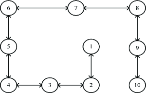
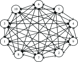
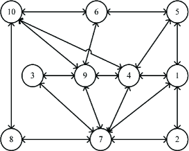
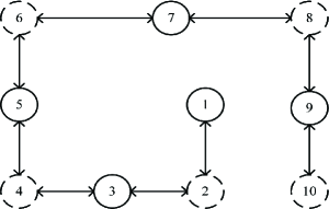
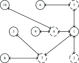
Figure 2: The original graphs and their corresponding simplest bipartite graphs. Top: original graphs (Left: line graph; Middle: fully connected graph; Right: random graph); Bottom: obtained simplest bipartite graphs (Left: The simplest bipartite graph of the line graph; Middle: The simplest bipartite graph of the fully connected graph; Right: The simplest bipartite graph of the random graph). The circles with solid lines denote nodes belonging to the index set $H$, and those with dashed lines denote nodes belonging to $T$.

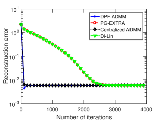
(a) Random graph.

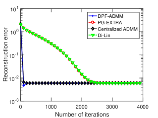
(b) Line graph.

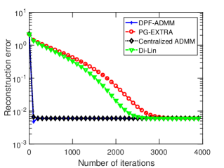
(c) Fully connected graph.

Figure 3: $\ell_{2}$+$\ell_{1}$ compressed sensing: reconstruction errors vs. the number of iterations for respective algorithms.

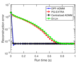
(a) Random graph.

(b) Line graph.

(c) Fully connected graph.

Figure 4: $\ell_{2}$+$\ell_{1}$ compressed sensing: reconstruction errors vs. run time for respective algorithms.

VI-A Smooth+nonsmooth: $\ell_{1}+\ell_{2}$ compressed sensing problem

We first consider the following decentralized $\ell_{1}$+$\ell_{2}$ compressed sensing problem:

$$\min_{\boldsymbol{x}} \quad\sum_{i=1}^{l}\frac{1}{{2\eta}}\left\|{{\boldsymbol{M}_{i}}{\boldsymbol{x}}-\boldsymbol{b}_{i}}\right\|_{2}^{2}+{{{\left\|{\boldsymbol{x}}\right\|}_{1}}}$$ (41)

where $\eta=1.2\times 10^{-4}$, $\boldsymbol{b}_{i}=\boldsymbol{M}_{i}\boldsymbol{x}+\boldsymbol{e}_{i}$ denotes the measurements held by each node, $\boldsymbol{M}_{i}\in{\mathbb{R}^{{m_{i}}\times n}}$ is the sensing matrix used by each node, and $\boldsymbol{e}_{i}$ denotes the associated noise vector. In our simulations, we set $m_{i}=3$, $n=100$, the sparsity level of the sparse signal $\boldsymbol{x}$ is set equal to 5. Entries of the measurement matrix and the noise vector are i.i.d Gaussian random variables. The variance of the entry in the noise vector is set to $10^{-3}$.

We compare our proposed algorithm with the PG-EXTRA [28] and the distributed linearized ADMM (Di-Lin) [36]. The PG-EXTRA and the Di-Lin are state-of-the-art algorithms recently designed for smooth+nonsmooth type of decentralized composite optimization problems. A centralized ADMM (Section $7$ in [2]) is also included in our experiments for comparison. The centralized ADMM assumes a star topology in which all nodes are individually connected to a central point and there is no connection among local nodes. The consensus for the centralized ADMM is achieved by letting each local variable equal to an extra variable $\boldsymbol{z}$ held by the central node, i.e. $\boldsymbol{x}_{i}=\boldsymbol{z}$, $1\leq i\leq l$. In each iteration, the local node computes a new $\boldsymbol{x}_{i}$ and sends it to the central node, and the central node updates $\boldsymbol{z}$ based on the received $\{\boldsymbol{x}_{i}\}$. The updated $\boldsymbol{z}$ is then sent back to all local nodes. It is widely acknowledged [28] that the centralized ADMM usually provides better performance than decentralized methods. Fig. 3 plots the reconstruction errors vs. the number of iterations for respective algorithms. Results are averaged over $10^{3}$ independent runs, with the noise randomly generated for each run. We see that our proposed method achieves a much faster convergence rate than the PG-EXTRA and the Di-Lin: it takes PG-EXTRA and Di-Lin more than $2000$ iterations to converge (the PG-EXTRA and the Di-Lin achieve similar performance), whereas only about $200$ iterations are needed for our algorithm to converge. Such a performance improvement is primarily due to the fact that our proposed method does not need to resort to any proximal term which is known to slow down the convergence speed. Notably, the proposed DPF-ADMM achieves performance almost the same as that of the centralized ADMM. This result shows the effectiveness and superiority of our proposed method. Also, since our proposed method operates over a simplest bipartite graph with a minimum number of edges, the amount of data to be exchanged (among nodes) per iteration is considerably reduced compared with the competing algorithms. Such a merit makes our proposed algorithm particularly suitable for networks which are subject to stringent power and communication constraints.

To more fairly evaluate the computational complexity of respective algorithms, in Fig. 4, we depict the reconstruction errors as a function of the average run time (in seconds). We see that it takes less time for our proposed method to converge than the PG-EXTRA and the Di-Lin.

VI-B Nonsmooth+nonsmooth: $\ell_{1}+\ell_{1}$ compressed sensing problem

Next we consider the $\ell_{1}$+$\ell_{1}$ compressed sensing problem:

$$\min_{\boldsymbol{x}} \quad\sum_{i=1}^{l}\frac{1}{\eta}\|\boldsymbol{M}_{i}\boldsymbol{x}-\boldsymbol{b}_{i}\|_{1}+\|\boldsymbol{x}\|_{1}$$ (42)

where $\eta$ is set to $1.2\times 10^{-3}$, and $\boldsymbol{M}_{i}$ is the same as before. Each noise vector $\boldsymbol{e}_{i}$ has only one nonzero entry, which is a Gaussian random variable whose variance is $10^{-2}$. Note that the proximal mapping of $\|\boldsymbol{x}\|_{1}$ has a closed form solution. Nevertheless, the proximal mapping of $\|\boldsymbol{M}_{i}\boldsymbol{x}-\boldsymbol{b}\|_{1}$ does not have a closed form solution. In this case, we need to transform the problem (42) into a form that can be handled by our proposed method. We introduce an auxiliary variable to (42):

$$\min_{\boldsymbol{x},\boldsymbol{u}} \sum_{i=1}^{l}\frac{1}{\eta}\|\boldsymbol{u}\|_{1}+\phi(\boldsymbol{u}-\boldsymbol{M}_{i}\boldsymbol{x}-\boldsymbol{b}_{i})+\|\boldsymbol{x}\|_{1}$$ (43)

where $\phi(\boldsymbol{x})$ is an indicator function, whose value is $+\infty$ if $\boldsymbol{x}\neq\boldsymbol{0}$, and $\boldsymbol{0}$ otherwise. Let $f_{i}(\boldsymbol{x};\boldsymbol{u})=\frac{1}{\eta}\|\boldsymbol{u}\|_{1}+\phi(\boldsymbol{u}-\boldsymbol{M}_{i}\boldsymbol{x}-\boldsymbol{b}_{i})$ and $g_{i}(\boldsymbol{x})=\|\boldsymbol{x}\|_{1}$, then the problem (43) can be written as

$$\min_{\boldsymbol{x},\boldsymbol{u}} \quad\sum_{i=1}^{l}f_{i}(\boldsymbol{x};\boldsymbol{u})+g_{i}(\boldsymbol{x})$$ (44)

which is similar to (2). Following the derivation in Section V, the decentralized formulation of the problem (44) can be described as

$$\mathop{\min}\limits_{{\tilde{\boldsymbol{x}}}_{f},{\tilde{\boldsymbol{u}}}_{f}\ {\tilde{\boldsymbol{y}}}_{g}} \quad\tilde{f}({\tilde{\boldsymbol{x}}}_{f};{\tilde{\boldsymbol{u}}}_{f})+\tilde{g}({\tilde{\boldsymbol{y}}}_{g})$$

s.t. $$\quad\boldsymbol{C}_{H}{\tilde{\boldsymbol{x}}}_{f}+\boldsymbol{C}_{T}{\tilde{\boldsymbol{y}}}_{g}=\boldsymbol{0}$$ (45)

where all the notations except ${\tilde{\boldsymbol{u}}}_{f}^{T}=[{\tilde{\boldsymbol{u}}}_{H}^{T}\ {\tilde{\boldsymbol{u}}}_{T}^{T}]^{T}$ is the same as those in Section V. Note that the variable ${\tilde{\boldsymbol{u}}}_{f}$ is kept locally by each node and does not participate in the information exchange. It is difficult to handle the indicator function and the $\ell_{1}$ norm in $\tilde{f}$ simultaneously, as a compromise, we choose to rewrite the indicator function as an equality constraint. Attaching an additional Lagrangian multiplier to the this equality constraint, now we can apply our proposed DPF-ADMM to solve (45).

Most existing decentralized algorithms are designed exclusively for solving smooth+nonsmooth problems, including the PG-EXTRA. Thus, we choose to compare our proposed algorithm with the DGD [17] and the centralized ADMM. For the competing algorithms, the parameters are tuned to achieve the best performance. Fig. 5 plots reconstruction errors vs. the number of iterations for respective algorithms. Results are averaged over $10^{4}$ runs, with the noise randomly generated for each run. We see that the our proposed DPF-ADMM presents a significant performance advantage over the DGD in terms of both reconstruction accuracy and convergence speed. Due to the simple structure, the computation time (per iteration) of the DGD is about half of that of our proposed algorithm. Nevertheless, the DPF-ADMM still exhibits an overwhelming advantage over the DGD in terms of the computational complexity, see Fig. 6.

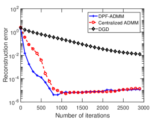
(a) Random graph.

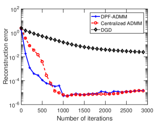
(b) Line graph.

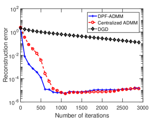
(c) Fully connected graph.

Figure 5: $\ell_{1}+\ell_{1}$ compressed sensing: reconstruction errors vs. the number of iterations for respective algorithms.

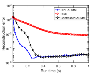
(a) Random graph.

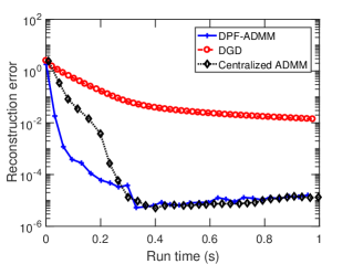
(b) Line graph.

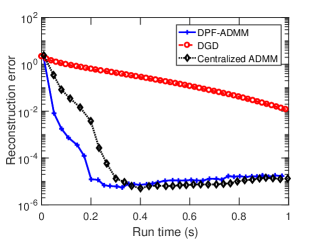
(c) Fully connected graph.

Figure 6: $\ell_{1}+\ell_{1}$ compressed sensing: reconstruction errors vs. average run time for respective algorithms.

VII Conclusion

In this paper, we proposed a decentralized proximal-free ADMM for solving decentralized composite optimization problems. The proposed algorithm was developed based on a simplest bipartite graph, which is defined as a bipartite graph that has a minimum number of edges to keep the graph connected. We showed that the simplest bipartite graph has some interesting properties that can be utilized to develop a decentralized algorithm without involving any proximal terms. The proposed algorithm exhibits a much faster convergence speed than state-of-the-art decentralized algorithms. Notably, it achieves performance similar to that of the centralized ADMM, which is known to provide the best achievable performance for all decentralized methods. In addition, the proposed algorithm entails a minimal communication cost because it runs on a simplest bipartite graph, which has the minimum number of edges that keeps the graph connected.

Appendix A Proof of Lemma 2

To prove that the matrix $\boldsymbol{X}$ has full row rank, we only need to show that the dimension of the null space of $\boldsymbol{X}^{T}$ is equal to one because $\boldsymbol{X}$ is an $(l-1)\times l$ matrix. From Lemma 1, we know that each row of $\boldsymbol{X}$ has only two nonzero elements that are of equal magnitude but opposite signs. Therefore it is clear that an all-one column vector $\boldsymbol{1}$ lies in the null space of $\boldsymbol{X}^{T}$, i.e. $\boldsymbol{X}\boldsymbol{1}=\boldsymbol{0}$. On the other hand, in the following, we show that for any vector $\boldsymbol{z}\notin\text{span}\{\boldsymbol{1}\}$, we have $\boldsymbol{X}\boldsymbol{z}\neq\boldsymbol{0}$.

For any vector $\boldsymbol{z}\notin\text{span}\{\boldsymbol{1}\}$, we can always find two entries of $\boldsymbol{z}$, say, $z_{i}$ and $z_{j}$, that are nonidentical, i.e. $z_{i}\neq z_{j}$. Suppose there is an edge between node $i$ and node $j$ in the simplest bipartite graph, and let $\boldsymbol{x}^{T}$ denote the row in $\boldsymbol{X}$ corresponding to this edge. According to the results in Lemma 1, we know that the $i$th and $j$th entries of $\boldsymbol{x}^{T}$ have a magnitude of $1$ but opposite signs, whereas other entries equal to zero. In this case, we have $\boldsymbol{x}^{T}\boldsymbol{z}\neq 0$, which implies $\boldsymbol{X}\boldsymbol{z}\neq\boldsymbol{0}$. Now consider the case where there is no direct link (i.e. edge) between node $i$ and node $j$. We first assume $\boldsymbol{X}\boldsymbol{z}=\boldsymbol{0}$ and proceed our proof by contradiction. Since the simplest bipartite graph is a connected graph, there always exists a route to connect these two nodes. Suppose there are $s$ intermediate nodes, say node $k_{1}$, $\ldots$, $k_{s}$, between node $i$ and node $j$. Since there is an edge between node $i$ and node $k_{1}$, its corresponding row in $\boldsymbol{X}$, denoted as $\boldsymbol{x}_{t_{1}}^{T}$, has two nonzero entries (i.e. the $i$th entry and the $k_{1}$th entry) of equal magnitude but opposite signs. From $\boldsymbol{X}\boldsymbol{z}=\boldsymbol{0}$, we can arrive at $z_{i}=z_{k_{1}}$. Following a similar derivation, we can establish a sequence of equations: $z_{k_{1}}=z_{k_{2}},\ldots,z_{k_{s}}=z_{j}$. Combining these equations, we eventually reach the conclusion that $z_{i}=z_{j}$, which contradicts our original assumption $z_{i}\neq z_{j}$. Therefore $\boldsymbol{X}\boldsymbol{z}=\boldsymbol{0}$ cannot be true. In other words, for any vector $\boldsymbol{z}\notin\text{span}\{\boldsymbol{1}\}$, we have $\boldsymbol{X}\boldsymbol{z}\neq\boldsymbol{0}$, which implies that the dimension of the null space of $\boldsymbol{X}^{T}$ is equal to one. Hence $\boldsymbol{X}$ has full row rank.

References

• [1] R. Olfati-Saber, J. Fax, and R. Murray, “Consensus and cooperation in networked multi-agent systems,” Proceedings of the IEEE, vol. 95, no. 1, pp. 215–233, 2007.
• [2] S. Boyd, N. Parikh, and E. Chu, “Distributed optimization and statistical learning via the alternating direction method of multipliers,” Foundations and Trends in Machine learning, vol. 3, no. 1, pp. 1–122, 2011.
• [3] Q. Ling and Z. Tian, “Decentralized sparse signal recovery for compressive sleeping wireless sensor networks,” IEEE Transactions on Signal Processing, vol. 58, no. 7, pp. 3816–3827, 2010.
• [4] W. Ren, R. Beard, and E. Atkins, “Information consensus in multivehicle cooperative control,” IEEE Control System Magazine, vol. 27, no. 2, pp. 71–82, 2007.
• [5] J. Meng, W. Yin, H. Li, E. Hossain, and Z. Han, “Collaborative spectrum sensing from sparse observations in cognitive radio networks,” IEEE Journal of Selected Areas on Communications, vol. 29, pp. 327–337, 2011.
• [6] G. Giannakis, N. Gatsis, V. Kekatos, S. Kim, H. Zhu, and B. Wollenberg, “Monitoring and optimization for power systems: A signal processing perspective,” IEEE Signal Processing Magazine, vol. 30, pp. 107–128, 2013.
• [7] K. Zhou and S. Roumeliotis, “Multirobot active target tracking with combinations of relative observations,” IEEE Transactions on Robotics, vol. 27, no. 4, pp. 678–695, 2011.
• [8] P. Forero, A. Cano, and G. Giannakis, “Consensus-based distributed support vector machines,” Journal of Machine Learning Research, vol. 11, no. May, pp. 1663–1703, 2010.
• [9] F. Yan, S. Sundaram, and S. Vishwanathan, “Distributed autonomous online learning: Regrets and intrinsic privacy-preserving properties,” IEEE Transactions on Knowledge and Data Engineering, vol. 25, no. 11, pp. 2483–2493, 2013.
• [10] G. Giannakis, Q. Ling, and G. Mateos, “Decentralized learning for wireless communications and networking,” Splitting Methods in Communication, Imaging, Science, and Engineering. Springer, pp. 461–497, 2016.
• [11] J. Tsitsiklis, D. Bertsekas, and M. Athans, “Distributed asynchronous deterministic and stochastic gradient optimization algorithms,” IEEE Transactions on Automatic Control, vol. 31, no. 9, pp. 803–812, 1986.
• [12] D. Bertsekas, “Distributed asynchronous computation of fixed points,” Mathematical Programming, vol. 27, no. 1, pp. 107–120, 1983.
• [13] A. Nedić and D. Bertsekas, “Incremental subgradient methods for nondifferentiable optimization,” SIAM Journal on Optimization, vol. 12, no. 1, pp. 109–138, 2001.
• [14] A. Nedić, D. Bertsekas, and V. Borkar, “Distributed asynchronous incremental subgradient methods,” Studies in Computational Mathematics, vol. 8, pp. 381–407, 2001.
• [15] ——, “Incremental proximal methods for large scale convex optimization,” Mathematical Programming, vol. 129, no. 2, p. 163, 2011.
• [16] M. Gurbuzbalaban, A. Ozdaglar, and P. Parrilo, “On the convergence rate of incremental aggregated gradient algorithms,” SIAM Journal on Optimization, vol. 27, no. 2, pp. 1035–1048, 2017.
• [17] A. Nedić and A. Ozdaglar, “Distributed subgradient methods for multi-agent optimization,” IEEE Transactions on Automatic Control, vol. 54, no. 1, pp. 48–61, 2009.
• [18] S. Ram, A. Nedic, and V. Veeravalli, “Distributed stochastic subgradient projection algorithms for convex optimization,” Journal of Optimization Theory and Applications, vol. 3, no. 147, pp. 516–545, 2010.
• [19] A. Nedić, “Asynchronous broadcast-based convex optimization over a network,” IEEE Transactions on Automatic Control, vol. 56, no. 6, pp. 1337–1351, 2009.
• [20] D. Bajovic, D. Jakovetic, N. Krejic, and N. Jerinkic, “Newton-like method with diagonal correction for distributed optimization,” SIAM Journal on Optimization, vol. 27, no. 2, pp. 1171–1203, 2015.
• [21] A. Mokhtari, Q. Ling, and A. Ribeiro, “Network Newton distributed optimization methods,” IEEE Transactions on Signal Processing, vol. 65, no. 1, pp. 146–161, 2017.
• [22] A. Mokhtari, W. Shi, Q. Ling, and A. Ribeiro, “A decentralized second-order method with exact linear convergence rate for consensus optimization,” IEEE Transactions on Signal and Information Processing over Networks, vol. 2, no. 4, pp. 507–522, 2016.
• [23] G. Mateos, J. Bazerque, and G. Giannakis, “Distributed sparse linear regression,” IEEE Transactions on Signal Processing, vol. 58, no. 10, pp. 5262–5276, 2010.
• [24] W. Shi, Q. Ling, K. Yuan, G. Wu, and W. Yin, “On the linear convergence of the ADMM in decentralized consensus optimization,” IEEE Transactions on Signal Processing, vol. 62, no. 7, pp. 1750–1761, 2014.
• [25] T. Chang, M. Hong, and X. Wang, “Multi-agent distributed optimization via inexact consensus ADMM,” IEEE Transactions on Signal Processing, vol. 63, no. 2, pp. 482–497, 2014.
• [26] J. Xu, S. Zhu, and Y. Soh, “A forward backward bregman splitting scheme for regularized distributed optimization problems,” IEEE Conference on Decision and Control, pp. 1093–1098, 2016.
• [27] D. Meng, M. Fazel, and M. Mesbahi, “Proximal alternating direction method of multiplier for distributed optimization on weighted graphs,” IEEE Conference on Decision and Control, vol. 63, no. 2, pp. 482–497, 2015.
• [28] W. Shi, Q. Ling, G. Wu, and W. Yin, “Extra: An exact first-order algorithm for decentralized consensus optimization,” SIAM Journal on Optimization, vol. 25, no. 2, pp. 944–966, 2015.
• [29] B. Wang, H. Jiang, J. Fang, and H. Duan, “A proximal ADMM for decentralized composite optimization,” IEEE Signal Processing Letters, vol. 25, no. 8, pp. 1121–1125, 2018.
• [30] W. Shi, Q. Ling, G. Wu, and W. Yin, “A proximal gradient algorithm for decentralized composite optimization,” IEEE Transactions on Signal Processing, vol. 63, no. 22, pp. 6013–6023, 2015.
• [31] C. Godsil and G. Royle, “Algebraic graph theory,” Springer, 2001.
• [32] R. Olfati-Saber, J. Fax, and R. Murray, “A fast iterative shrinkage-thresholding algorithm for linear inverse problems,” SIAM Journal on Imaging Sciences, vol. 2, no. 1, pp. 183–202, 2009.
• [33] R. Prim, “Shortest connection networks and some generalizations,” Bell System Technical Journal, vol. 36, no. 6, pp. 1389–1401, 1957.
• [34] J. Kruskal, “On the shortest spanning subtree of a graph and the traveling salesman problem,” Proceedings of the American Mathematical Society, vol. 1, no. 1, pp. 48–50, 1956.
• [35] C. Chen, B. He, and Y. Ye, “The direct extension of ADMM for multi-block convex minimization problems is not necessarily convergent,” Mathematical Programming, vol. 155, no. 1, pp. 57–79, 2016.
• [36] N. Aybat, Z. Wang, T. Lin, and S. Ma, “Distributed linearized alternating direction method of multipliers for composite convex consensus optimization,” IEEE Transactions on Automatic Control, vol. 63, no. 1, pp. 5–20, 2018.