Distributed-Memory Forest-of-Octrees Raycasting

.

Abstract

We present an MPI-parallel algorithm for the in-situ visualization of computational data that is built around a distributed linear forest-of-octrees data structure. Such octrees are frequently used in element-based numerical simulations; they store the leaves of the tree that are local in the curent parallel partition.

We proceed in three stages. First, we prune all elements whose bounding box is not visible by a parallel top-down traversal, and repartition the remaining ones for load-balancing. Second, we intersect each element with every ray passing its box to derive color and opacity values for the ray segment. To reduce data, we aggregate the segments up the octree in a strictly distributed fashion in cycles of coarsening and repartition. Third, we composite all remaining ray segments to a tiled partition of the image and write it to disk using parallel I/O.

The scalability of the method derives from three concepts: By exploiting the space filling curve encoding of the octrees and by relying on recently developed tree algorithms for top-down partition traversal, we are able to determine sender/receiver pairs without handshaking and/or collective communication. Furthermore, by partnering the linear traversal of tree leaves with the group action of the attenuation/emission ODE along each segment, we avoid back-to-front sorting of elements throughout. Lastly, the method is problem adaptive with respect to the refinement and partition of the elements and to the accuracy of ODE integration.

Carsten Burstedde, 2018.

The author acknowledges travel support by the Hausdorff Center for Mathematics (HCM) at the Rheinische Friedrich-Wilhelms-Universität Bonn, Germany.

1 Introduction

2 Visualization Model

In this section we begin with defining the geometry of the domain, the camera’s position and properties, and introduce the setup for casting rays through the geometry to the projection plane. We focus in detail on the mathematical model for propagating light along a ray and computing attenuation and emission. Beginning with the well-known ordinary differential equation (ODE), we propose the notion of a ray segment that represents the exact effect of the medium along its length. We develop the group properties of the ODE’s solution into a formalism that allows to combine, cut, and average arbitrary segments. Whether segments are separate, touching, or overlapping, the formalism preserves the physics exactly, which allows us to aggregate all segments of the ray into the final pixel without requiring global back-to-front processing. We will rely on this property throughout the paper.

2.1 Domain description

We assume that the geometry to be visualized is contained in a space-forest, that is, a collection of space-trees $\{t_{k}\}$. Each quad- or octree $t_{k}$ defines an adaptive subdivision of the $d$-dimensional reference hypercube into its leaves (we use the terms leaf and element interchangeably). Each node in the tree is either a leaf or the root of a (sub)tree, and we refer to the union of elements as the mesh.

The data to be visualized may either have been computed in this same forest, or it may originate from a different source that is covered by the forest and accessible by element. We also assume that the space-forest is partitioned in parallel: Each element and the data it covers is available on exactly one process. Thus, each element has precisely one owner process, which relates to its owned elements as the local ones.

We create two- or three-dimensional manifolds by allowing for smooth transformations

$$\mathbf{j}_{k}:[0,1]^{d}\rightarrow D_{k}\subset\mathbb{R}^{3}$$ (2.1)

of the reference hypercube into each of the tree’s domains $D_{k}$ in real space. Thus, we define a separate transformation for each tree, which is then inherited by all elements of a tree. We can also speak of the reference cube for an individual element, which is simply a subcube. All transformations must be compatible in such a way that $\cup_{k}D_{k}$ makes up the complete geometry. This approach allows us to define the geometry with relatively few parameters compared to storing an independent transformation for each element. Usually it is possible to replicate the geometry parameters globally, while there are far too many elements to replicate the mesh in parallel. If needed, there are ways to avoid replicating per-tree data as well [Burstedde and Holke (2017)].

In our application we define each transformation $\mathbf{j}_{k}$ as the tensor product of degree-$R$ Lagrange polynomials $\psi_{m}(t)$, $m=0,\ldots,R$. For numerical stability, we choose Gauß-Lobatto nodes $\eta_{m}\in[0,1]$ as the nodes of the basis polynomials, which means that

$$\psi_{m}(\eta_{m^{\prime}})=\delta_{mm^{\prime}}.$$ (2.2)

The image of the $d$-dimensional unit cube is defined by $(R+1)^{d}$ control points $\mathbf{z}_{m_{1},\ldots,m_{d}}$. We derive these points per-tree from any a-priori definition of the geometry (e.g., a CAD system), producing the formula

$$\mathbf{j}_{k}(t_{1},\ldots,t_{d})=\sum_{m_{1},\ldots,m_{d}=0}^{R}\mathbf{z}_{k;m_{1},\ldots,m_{d}}\psi_{m_{1}}(t_{1})\cdots\psi_{m_{d}}(t_{d}).$$ (2.3)

This expression is legal in affine space since Lagrange polynomials form a partition of unity,

$$\sum_{m_{1},\ldots,m_{d}=0}^{R}\psi_{m_{1}}(t_{1})\cdots\psi_{m_{d}}(t_{d})=\sum_{m_{1}}\psi_{m_{1}}(t_{1})\cdots\sum_{m_{d}}\psi_{m_{d}}(t_{d})=1,\quad t_{1},\ldots,t_{d}\in\mathbb{R},$$ (2.4)

such that translating points commutes with translating the domain.

Gauß-Lobatto nodes have the property that $\eta_{0}=0$, $\eta_{N}=1$. Together with the nodality (2.2) this implies that the shape of a tree’s boundary face, edge, or vertex is defined by the control points on that part of the boundary alone. The key observation is that the geometry of a tree’s face in three dimensions has the structure of (2.3) reduced to dimension two, using a strict subset of the control points.

To visualize two-dimensional manifolds, we need to intersect a straight line with the image of an element’s reference square under the transformation $\mathbf{j}_{k}$. This produces a certain number of intersection points, usually none or zero (but maybe more for non-affine transformations) that we use to update the color information for that ray. For three-dimensional manifolds we intersect a ray with each of the faces of an element and connect the intersection points by a path through the element. Then we update the ray’s color information by sampling the elements’ properties along the path segments.

We emphasize that for either two or three space dimensions, the intersection routine is the same, using (2.3) with $d=2$. We touch on the mathematical details in Appendix A.1. We also note that it would be possible to use a different type of geometry transformation altogether, as long as the intersecton of a two-dimensional mapped square with a ray can be computed analytically or numerically.

When we have a non-affine geometry transformation, an element may produce multiple path segments that intermix with those from neighboring elements. Beginning with Section 2.3 below, we propose a way of supporting this without introducing dependencies between any two elements.

2.2 Camera setup

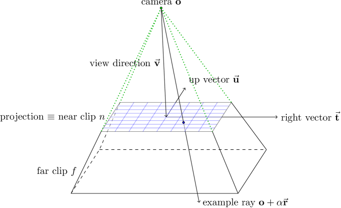
Figure 1: Our conventions for the camera setup. The projection rectangle is divided into pixels (blue), where each pixel is associated with a ray through its center. The view frustum lies between the near and far clipping planes (at distances $n$ and $f$ from the camera) and the sides of the pyramid stump. The (left-handed) camera coordinate system is defined by the unit right and up-vectors and the normalized view direction, $(\vec{\mathbf{t}},\vec{\mathbf{u}},\vec{\mathbf{v}}/n)$, with the origin $\mathbf{o}$ at the camera. A ray with the pixel coordinates $(i,j)$ has the direction vector $\vec{\mathbf{r}}$ given by equation (2.5). The ray coordinate is $\alpha\geq 0$, where $\alpha=0$ identifies the camera and $\alpha=1$ the intersection of the ray with its pixel’s center.

In this paper, we use a standard way of defining the camera (see Figure 1). The camera is defined by a point location in space $\mathbf{o}$, a view direction $\vec{\mathbf{v}}$, and a projection/image rectangle perpendicular to the view direction. The rectangle has two principal axes defined by the unit vectors $\vec{\mathbf{t}}$ (right) and $\vec{\mathbf{u}}$ (up) that are thought to originate at its center $\mathbf{o}+\vec{\mathbf{v}}$. Thus, the distance $n$ of the projection rectangle from the camera is $n=\lVert\vec{\mathbf{v}}\rVert$. The rectangle is logically divided into a $w\times h$ grid of pixels, each having length $\ell$ in the projection plane. The pixels are indexed by zero-based integers $(i,j)$. Each pixel is associated with a ray that connects the camera with its center point and extends beyond the projection plane. The ray is thus a set of points along a line parameterized by $\alpha\geq 0$,

$$\mathbf{o}+\alpha\vec{\mathbf{r}},\qquad\text{where}\qquad\vec{\mathbf{r}}=\vec{\mathbf{v}}+\ell\left(\left(i-\frac{w-1}{2}\right)\vec{\mathbf{t}}+\left(j-\frac{h-1}{2}\right)\vec{\mathbf{u}}\right).$$ (2.5)

The unit vector in the view direction is $\vec{\mathbf{v}}/n$. We also define near and far clipping planes, where we identify the near clipping plane with the projection plane for convenience. The distances from the camera are thus the aforementioned $n$ for the near plane and $f>n$ for the far plane. The visible volume is contained in the view frustum defined by the clipping planes and the four lines that connect the camera with each of the corners of the projection rectangle.

To compute the ray intersections with the geometry, it is convenient to transform all geometry locations into the camera system, where the view direction is aligned with the negative $z$ axis. Formally, this camera-aligned geometry transformation is defined as

$$\mathbf{X}=\Phi(\mathbf{x})=(\vec{\mathbf{t}},\vec{\mathbf{u}},\vec{\mathbf{v}}/n)^{T}\left(\mathbf{x}-\mathbf{o}\right).$$ (2.6)

After this affine-orthogonal transformation, the visible $z$ values lie in $[n,f]$.

We can avoid the computational expense that is seemingly associated with this calculation: Due to our definition of the geometry as per-tree transformations, it suffices to transform each of the per-tree control points into the camera system. Examining (2.3) and using (2.4), we establish that the camera-aligned geometry transformation is given by

$$\mathbf{J}_{k}=\Phi\circ\mathbf{j}_{k}\qquad\Leftrightarrow\qquad\mathbf{Z}_{k;m_{1},\ldots,m_{d}}=\Phi(\mathbf{z}_{k;m_{1},\ldots,m_{d}}).$$ (2.7)

This mechanism effectively changes the per-element transformations as desired and can be performed in a preprocessing stage before executing the actual visualization.

Below, we optimize the visibility tests for an element by bounding box checks. Bounding boxes are computed axis-aligned (abbreviated AABB) with respect to the camera system by subjecting a subtree’s reference domain to its tree’s camera-aligned geometry transformation $\mathbf{J}_{k}$ and then computing the minima and maxima of its extent in each coordinate direction. For high order geometry transformations this is non-trivial and may be accelerated by computing a more lenient approximate criterion instead. Once we know this 3D brick in camera coordinates, we project it into the image plane to determine the equivalent pixel rectangle, which is our (2D) AABB.

2.3 Computing ray segments

In a classic raycasting procedure, each ray is thought to originate at infinity and followed to the camera location, intersecting a projection plane somewhere in between. Along its path, the ray aggregates color information by passing through the geometry. Each ray can be divided into a number of line segments defined by the ray’s intersection with the elements of the geometry, or in other words the leaves of the data tree. The usual way of rendering the ray is to initialize it with a background color or transparency and to begin with the segment farthest away from the camera. The segment modifies the color values seen, which are then processed with the second-farthest segment and so on, back to front. Processing a ray in this sequence guarantees that opacity and color values are computed correctly, but enforces a sequential processing of segments.

In this paper we reformulate the rendering of a ray such that we can process the segments in any sequence. We define the fundamental operation of aggregating two neighboring ray segments into a longer, equivalent one. Once we have aggregated all segments, we can process the background color through the last effective segment and achieve an identical result as with the classic procedure. All we require is that the aggregation is an associative mathematical operation, which may limit the general class of rendering methods but applies to the examples discussed here. In a sense, we can work with a local instead of a global view of the ray.

Our specific ray model takes into account emission and absorption separately for each color channel. Suppose a channel’s emission coefficient along a line in real space parameterized by $x\in\mathbb{R}$ is $\gamma(x)$ in units of intensity over length, and the absorption coefficient is $\beta(x)$ in units of one over length. This leads to the ordinary differential equation (ODE)

$$I^{\prime}(x)=\gamma(x)-\beta(x)I(x)$$ (2.8)

with known solution

$$I(x)=A(x)I(x_{1})+B(x),$$ (2.9)

where $x_{1}$ is arbitrary and

$$A(x)=e^{\int_{x_{1}}^{x}-\beta(x^{\prime})\mathrm{d}x^{\prime}},\qquad B(x)=A(x)\int_{x_{1}}^{x}\frac{\gamma(x^{\prime})}{A(x^{\prime})}\mathrm{d}x^{\prime}.$$ (2.10)

Writing $I_{i}=I(x_{i})$ and evaluating the solution at $x_{2}=x_{1}+\Delta x$, we obtain the affine-linear formula

$$I_{2}=AI_{1}+B$$ (2.11)

depending on the two numbers $(A,B)=f(\beta,\gamma)$,

$$A=A(x_{2})=e^{-\int_{x_{1}}^{x_{2}}\beta(x^{\prime})\mathrm{d}x^{\prime}},\qquad B=B(x_{2})=\int_{x_{1}}^{x_{2}}\gamma(x)e^{-\int_{x}^{x_{2}}\beta(x^{\prime})\mathrm{d}x^{\prime}}\mathrm{d}x.$$ (2.12)

The transmission ratio $A$ is dimensionless, while $B$ is the intensity added by emission. $A$ is always positive by construction. The special case of a transparent medium, $\beta(x)=0$, amounts to $A=1$ and $B=\int\gamma(x)\mathrm{d}x$.

The formulas simplify for constant $\beta$ and $\gamma$, which yield

$$A=e^{-\beta\Delta x},\qquad B=\frac{\gamma}{\beta}\left(1-A\right).$$ (2.13)

The mathematical limit for $\beta=0$ is well defined due to the relation $1-\exp(-\epsilon)\approx\epsilon$, which produces $B=\gamma\Delta x$.

We can thus uniquely identify a segment with the tuple $T$ consisting of the pixel index, the in and out coordinates $x_{i}$, and the characteristic values $(A,B)$ for each channel. This information corresponds to the exact physics.

2.4 Aggregating ray segments

Supposing that we have two adjacent segments characterized by $(A_{1},B_{1})$ for the farther one and $(A_{2},B_{2})$ for the one closer to the camera, it follows from (2.11) that they are equivalent to the segment

$$(A,B)=(A_{2},B_{2})\oplus(A_{1},B_{1})=(A_{2}A_{1},B_{2}+A_{2}B_{1}).$$ (2.14)

Theorem 1

The aggregation formula (2.14) is associative. Indeed, the segments $(A,B)$ form a non-abelian group $\mathcal{S}$ with identity $(1,0)$ and inverse

$$\ominus(A,B)=(1/A,-B/A).$$ (2.15)

Proof 2.1.

It suffices to show that $\mathcal{S}=(\mathbb{R}_{+}\times\mathbb{R},\oplus)$ is the semi-direct product of two groups with a non-trivial map $\theta$. We propose

$$\mathcal{A}=(\mathbb{R}_{+},\cdot),\qquad\mathcal{B}=(\mathbb{R},+),\qquad\mathcal{S}=\mathcal{A}\ltimes_{\theta}\mathcal{B}$$ (2.16)

with the group homomorphism $\theta:\mathcal{A}\to\operatorname{\mathrm{Aut}}(B)$ defined by

$$\theta(A)=(B\mapsto AB).$$ (2.17)

The formula for the inverse is inherited from this definition. Alternatively, the associativity, the identity element, and (2.15) are verified by inserting into (2.14).

We can use equation (2.14) any number of times to aggregate adjacent segments into equivalent larger ones without the need to proceed back-to-front globally. The segments do not need to touch if they are separated only by empty space.

The aggregation equation (2.14) is also useful when the emission and absorption coefficients are modeled as piecewise constant within an element, and we approximate the element’s effect on the ray by aggregating the sub-segments within each element. Due to the associativity, we can do this for any element without accessing other parts of the ray.

For a slight change of perspective, we may ask the question, which intensity $I$ follows from constant absorption and emission coefficients? We postulate the equilibrium $I=AI+B$ and insert (2.13), which yields

$$I=\frac{\gamma}{\beta}\qquad\text{or equivalently}\qquad B=B(A,I)=I(1-A).$$ (2.18)

Thus, we can interface the visualization code to an element-based application in a modular way, following any of two variants:

• The visualization code computes $x_{i}$ etc. for a segment by intersecting a ray with an element and passes it to the application.

• For each color channel, the application computes (or approximates) $A$ from its internal absorption model using the segment’s geometry. Now, there are two choices:

  1. The application computes (or approximates) $B$ from (2.12) or (2.13).

  2. The application computes $I$ as the desired intensity, e.g., by applying a transfer function to the data. Then it computes $B$ from $I$ by (2.18).

• The visualization code accepts $(A,B)$ and stores the tuple for future aggregation of this segment with other segments.

We recall that the approximation of $A$ by numerical integration is rather straightforward, while that of $B$ is less so. The alternative (2) thus removes a fairly complex computation from the application, possibly trading in some physical accuracy. As mentioned above, we can enhance the accuracy of this procedure by subsampling an element with multiple pieces of the ray segment. We will discuss proper numerical procedures that deliver provable error bounds in Section 2.7.

Once all segments of one ray are aggregated into final values indexed by the color channel, $(A_{i},B_{i})$, we can compute the visible intensity $I_{v,i}$ from the background intensity $I_{b,i}$ by

$$I_{v,i}=A_{i}I_{b,i}+B_{i}.$$ (2.19)

The intensity values $I_{v,i}$ are then converted into pixel RGB values. We see that writing an image with a transparency value is straightforward without background and emission, that is, when $I_{b,i}=1$ and $B_{i}=0$. Within a generic rendering framework, $A_{i}$ and $B_{i}$ can be fed into its routines for alpha blending.

2.5 Cutting and overlapping segments

Since some geometrical inaccuracies are often present in practice, it may occur that we create two partially overlapping segments for the same ray. We can resolve this situation by cutting the segments into pieces to isolate the overlapping section and then averaging the segment values in the overlapping interval. The first operation required is the split of one segment into two shorter equivalent ones of given lengths, say $\Delta x_{2}+\Delta x_{1}=\Delta x$. Inserting these values into (2.13) leads to

Theorem 2.

We split a segment with values $(A,B)$ into two segments $(A_{i},B_{i})$, $i=1,2$, according to

$$A_{i}=A^{\Delta x_{i}/\Delta x},\qquad B_{i}=B\frac{1-A_{i}}{1-A}.$$ (2.20)

The special case $A=1$ leads to $A_{i}=1$ and $B_{i}=B\Delta x_{i}/\Delta x$.

Proof 2.2.

Above formula is consistent with (2.13) and correct in the limit $\beta\Delta x\rightarrow 0$. Aggregating the two segments using (2.14) yields the original segment $(A,B)$.

The second operation, computing the average of two segments over the same interval, can be thought of alternating between infinitesimally small pieces of each ray. This motivates

Theorem 3.

We average the segments $(A_{i},B_{i})$, $i=1,2$ using the geometric mean for $A$ and the arithmetic mean for $B$,

$$A=\sqrt{A_{1}A_{2}},\qquad B=\frac{1}{2}(B_{1}+B_{2}).$$ (2.21)

Proof 2.3.

If we divide the length of each segment by a number $2N$, according to (2.13) this amounts to values

$$\bar{A}_{i}=A_{i}^{\frac{1}{2N}},\qquad\bar{B}_{i}=B_{i}\frac{1-\bar{A}_{i}}{1-A_{i}}.$$ (2.22)

Aggregating these two by using (2.14) and the approximation $1-A^{q}\approx q(1-A)$ for $q\ll 1$ and $A^{q}$ near $1$, we obtain

$$\bar{A}=\sqrt{A_{2}A_{1}}^{\frac{1}{N}},\qquad\bar{B}=\frac{1}{2N}\left(B_{2}+A_{2}^{\frac{1}{2N}}B_{1}\right).$$ (2.23)

Aggregating $N$ of these results and taking the limit $N\to\infty$ yields the claim.

2.6 Additional properties of segments

We can express absorption and emission coefficients in terms of the ray segment’s values by computing $f^{-1}(A,B)$, where we use that $f$ is injective for constant $\beta(x)$ and $\gamma(x)$,

$$\beta=-\frac{\ln A}{\Delta x}\qquad\text{and}\qquad\gamma=\frac{\beta B}{1-A}.$$ (2.24)

The formula for $\gamma$ has a well-defined limit for $A\to 1$. This provides a mechanism to average non-constant $\beta(x)$, $\gamma(x)$ to constants that are physically equivalent, i.e., yield an identical action on the intensity:

1. Compute $(A,B)$ from the general solution (2.12) to any desired accuracy.

2. Compute the physical average by (2.24).

By inspecting the definition of $A(x)$, we see that this leads to the integral average for $\beta$ and a more complex formula for $\gamma$.

Similarly, the aggregation of two segments leads to the weighted averages

$$\beta\Delta x=\sum_{i=1}^{2}\beta_{i}\Delta x_{i}\qquad\text{and}\qquad\frac{\gamma}{\beta}w=\sum_{i=1}^{2}\frac{\gamma_{i}}{\beta_{i}}w_{i}$$ (2.25)

with $w=w_{2}+w_{1}$, specifically

$$w=1-A,\qquad w_{2}=1-A_{2},\qquad w_{1}=A_{2}(1-A_{1}).$$ (2.26)

Again, the emission coeficients $\gamma_{i}$ are convex combined if $\beta_{1}=\beta_{2}$ but not in general. In addition, this formula is not suitable for the common case $A=1$. Thus, it is easier in practice to work in terms of $(A,B)$.

From physical intuition, we can neutralize the effect of a segment by running through it backwards. We may also ask how to achieve such neutralization by modifying the absorption and emission coefficients.

Theorem 4.

Let us introduce the transformation that reverses the interval,

$$y(x)=x_{1}+x_{2}-x.$$ (2.27)

Swapping $x_{1}$ with $x_{2}$ in (2.12) yields the inverse segment (2.15). This result is reproduced by the identity

$$\ominus(A,B)=f(-\beta\circ y,-\gamma\circ y).$$ (2.28)

Proof 2.4.

Both the swap $x_{i}\leftarrow y(x_{i})$ and (2.28) are verified by substituting into (2.12).

For constant absorption and emission, the formula simplifies to just taking negative $\beta$ and $\gamma$. This is consistent with both (2.13) and (2.24).

Choosing negative coefficients is not only a mathematical possibility, but may be related to physical processes: A negative absorption coefficient $\beta$ represents a proportional amplification of light by the medium (laser physics), and a negative $\gamma$ represents an absolute absorption per length unit (inverse led). Naturally, the flipside of this flexibility are intensities that grow out of bounds or become negative, which must be accounted for in the final translation from intensity to pixel values.

2.7 Numerical approximation of segments

In the preceding sections, we have established the mathematical tools required to formulate our overall visualization procedure in Section 3. All that is required for an application is to produce values $(A,B)$ given a ray segment running from $x_{1}$ to $x_{2}$. We use this section to propose one way that is close to the true physics by prompting the application for values of $\beta(x)$ and $\gamma(x)$ at locations that are automatically decided by a user-provided accuracy requirement.

There are two mathematical approaches to compute the change of intensity caused by the medium along a ray segment. One is numerically solving the ODE (2.8), and the other is to integrating it analytically and evaluating the integral by quadrature. We discuss both here, beginning with the ODE solve.

Considering the reformulation (2.9), we find two independent ODEs

$$A^{\prime}(x)=-\beta(x)A(x),\qquad B^{\prime}(x)=\gamma(x)-\beta(x)B(x).$$ (2.29)

Choosing an explicit Runge-Kutta (RK) method with $M$ stages and coefficients $c_{i}$, $a_{ij}$, and $b_{j}$, we obtain the evaluation points

$$\xi_{i}=x_{1}+c_{i}\Delta x,\qquad i=0,\ldots,M-1$$ (2.30)

and the stage values

$$\bar{A}_{i}=1+\Delta x\sum_{j=0}^{i-1}a_{ij}\left(-\beta(\xi_{j})\bar{A}_{j}\right),\qquad\bar{B}_{i}=\Delta x\sum_{j=0}^{i-1}a_{ij}\left(\gamma(\xi_{j})-\beta(\xi_{j})\bar{B}_{j}\right).$$ (2.31)

When selecting subdiagonal-explicit RK methods, such as explicit Euler, Heun’s method of order 2 or 3, or classical RK4, the sums collapse to one entry containing $a_{i,i-1}$. The equations for the final values also have the form above when setting $a_{Mj}=b_{j}$, $j=0,\ldots,M-1$, and $a_{MM}=0$, which leads to $A=\bar{A}_{M}$, $B=\bar{B}_{M}$.

Explicit RK methods have a restriction on the interval $\Delta x$ to ensure stability. For the type of ODE (2.29), the limit is of the order $1/\beta$. While proceeding with the solve, we watch the evaluations for a condition $\Delta x\beta(\xi_{j})>c_{\mathrm{RK}}$. If it arises, we abandon this RK step and replace it with two RK steps, each with one half of the original length. We repeat this procedure recursively for a problem-adaptive solve, knowing that the recursion is guaranteed to terminate. The computation is numerically stable if, conservatively, $c_{\mathrm{RK}}\leq 1/2$. We may reduce $c_{\mathrm{RK}}$ further to improve the accuracy of the method with an error rate of $c_{\mathrm{RK}}^{M}$. The adaptive RK solve is shown in Algorithm 1.

Input: $\Delta x=x_{2}-x_{1}\geq 0$, stability parameter $c_{\mathrm{RK}}>0$

1 for $i=0,\ldots,M$ do

2       Compute RK stage $(\bar{A}_{i},\bar{B}_{i})$ by (2.31)

3       if $i>0$ and above computation evaluates $\Delta x\beta(\xi_{i-1})>c_{\mathrm{RK}}$ then

             $x_{1/2}=\frac{1}{2}(x_{1}+x_{2})$

              /* split at midpoint */

             return $\textbf{segeval}(x_{1/2},x_{2})\oplus\textbf{segeval}(x_{1},x_{1/2})$

              /* recursion */

4            

5       end if

6      

7 end for

return $(\bar{A}_{M},\bar{B}_{M})$

Algorithm 1 $(A,B)\leftarrow\textbf{segeval}(x_{1},x_{2})$ by adaptive ODE solve

To avoid the stability issue altogether, we may switch to an implicit RK method. For the Gauß method of $M=2$ stages and order 4, we find the evaluation points $\xi_{0/1}=\frac{1}{2}\pm\sqrt{3}/6$ and solve the RK system analytically for

$$A=\frac{1-a_{1}+a_{2}}{1+a_{1}+a_{2}},\qquad B=\frac{b_{1}+b_{2}}{1+a_{1}+a_{2}},$$ (2.32)

where

$$a_{1} =\Delta x\left(\beta(\xi_{0})+\beta(\xi_{1})\right)/4, a_{2} =\Delta x^{2}\beta(\xi_{0})\beta(\xi_{1})/12,$$ (2.33a)

$$b_{1} =\Delta x\left(\gamma(\xi_{0})+\gamma(\xi_{1})\right)/2, b_{2} =\Delta x^{2}\left(\beta(\xi_{0})\gamma(\xi_{1})-\beta(\xi_{1})\gamma(\xi_{0})\right)\sqrt{3}/12.$$ (2.33b)

This formula is bounded regardless of $\Delta x$, but we see that the limit of very large $\Delta x$ produces $A=1$ and a difference of intensities for $B$, both unphysical. Thus, we use the recursion in Algorithm 1 as before, which allows us to enforce accuracy with rate $c_{\mathrm{RK}}^{2M}$.

The approach by quadrature can be exemplified by using Simpson’s rule, characterized by $M=3$ and known locations $c_{i}$ and weights $b_{j}$, as a good compromise between simplicity, accuracy, and cost. Considering the closed form (2.12), we arrive at

$$A=\exp\Biggl{(}-\Delta x\sum_{j=0}^{2}b_{j}\beta(\xi_{j})\Biggr{)},\qquad B=\Delta x\left(b_{0}A\gamma(\xi_{0})+b_{1}\sqrt{A}\gamma(\xi_{1})+b_{2}\gamma(\xi_{2})\right).$$ (2.34)

A disadvantage is that the computation involves exponentials and is thus more expensive than the numerical ODE solve. An advantage is that $\Delta x$ may be arbitrarily large and the result stays physical. We recommended again to embed the quadrature formula into the recursion described above, since the accuracy control by $c_{\mathrm{RK}}^{M}$ remains valuable.

2.8 Visualization of surfaces

Surfaces can be understood as 2D manifolds idealized from very thin 3D objects. Thus, a surface has a single intersection point with a ray, unless the ray is parallel or the surface doubles back to meet the ray several times. To model the optical parameters of the surface, we assume a surface thickness $h\ll\Delta x$. The distance traveled inside the surface is $h/\cos(\phi)$, where $\phi$ is the angle between the ray and the surface normal at the intersection point. Since $h$ is so small, it is justified to assume constant coefficients $\beta$, $\gamma$ for the surface’s material.

If we prescribe a desired transparency factor $A_{s}$ and absolute intensity $I_{s}$ produced by the surface, we obtain the value $B_{s}$ by (2.18). This computation is independent of the actual thickness assumed. In other words, we are not required to choose any particular value for $h$, and the method is well defined for $h\to 0$. This approach extends to rendering opaque surfaces. Instead of trying to approximate the limit $\beta\to\infty$, we may directly set $A_{s}=0$ and $B_{s}=I_{s}$ with no change to the aggregation logic. To incorporate the angle, we rely once more on (2.13) and define

$$A_{\phi}=A_{s}^{1/\cos\phi},\qquad B_{\phi}=B(A_{\phi},I_{s}).$$ (2.35)

3 Visualization Algorithm

In this section we go through the different phases of the overall parallel visualization algorithm. As mentioned above, we assume that the scene is stored in distributed memory, where the partition is defined by that of the space-forest. The relevant scene data is available from the individual leaves. Each leaf is stored on precisely one process, on which it is local. It is remote to all other processes. These assumptions are naturally met when visualizing computational data in-situ, and can be established by parallel forest traversal algorithms in the case of discrete data such as point sets or constructive solid geometry (CSG) descriptions. We demonstrate one example for each type of data in Section 4.

We consider the MPI model of parallelization, identifying an MPI rank with a process. The algorithms we present still apply if we further partition each MPI rank between CPU cores and/or accelerator units, and use threads instead of processes. We generally expect that all subalgorithms run simultaneously on all processes. This includes the case when some processes may have no relevant data to process in one or more of the phases despite our efforts to load-balance.

We allow for multiple images created in one rendering, where each image instance may have a different camera definition and/or different rules for background/skybox data and attenuation and emission. Top-down traversals of the forest will continue until the last of the instances considers a leaf or subtree invisible. A node is invisible when its AABB falls out of the image area, or when it is so small that it is no longer hit by a single ray.

Due to the aggregation logic laid out in Section 2, we do not need to visit the elements in back-to-front ray order. Instead, we follow the space filling curve encoding the distributed mesh, which ensures linear and cache-friendly memory access. We assume that the total number of MPI processes is given and fixed, and that the user has specified another and usually smaller number of writer processes to store the images on disk using parallel I/O.

The main challenge in parallel is thus to transport the image information from the data-oriented partition of the input forest to the pixel-oriented partition of the output image. To this end, we propose the phases of reassigning the input data, rendering it into ray segments, aggregating the segments, and compositing them to pixels. Except for the actual rendering of segments, all phases require careful redistribution of data in parallel as described in the following.

3.1 Culling and pre-partition

The input forest is usually partitioned to equidistribute numerical data between the processes. Raycasting, on the other hand, will benefit from a parallel equidistribution of visible pixels. Since the most expensive operation in our visualization pipeline is the numerical integration of ray segments for each element (Section 2.7), it makes sense to reassign the data in parallel before rendering.

We render non-destructively, meaning that we treat the input as read-only. This first phase is to create a visualization forest (“vforest”) structure repartitioned by pixel count, copying only the data of the visible elements for the upcoming rendering step.

1. Initialize an empty vforest, e.g. using p4est_build [Burstedde (2018), Section 3].

2. Run a top-down traversal of the local input elements, e.g. using p4est_search_local [Isaac et al. (2015), Section 3], tracking which of the image instances consider a tree node visible.

   • Each tree node has multiple AABBs, one for each image instance. Whenever the AABB of a node falls outside of an image instance’s view or shrinks to zero pixels, that instance is removed from the list.

   • When the list is empty, that is, the AABB of the tree node has become invisible in all instances, the node is pruned from the recursion.

   • Whenever we reach a leaf, it is visible to at least one instance and we add it to the vforest and copy its element data.

3. Finalize the vforest by adding the smallest possible set of coarse invisible elements that make it a complete octree; this is still part of p4est_build.

4. Repartition the vforest, where each leaf has a weight proportional to its visible pixel count summed over all instances.

5. Communicate the data copied above to the new owner of its element, e.g. by calling the p4est_transfer functions [Burstedde (2018), Section 6].

The parallel forest build, repartitioning, and transfer of data are fast operations for an efficient forest-of-octree implementation, requiring only a fraction of a second. The run time of copying the visible element data will be proportional to the input set and generally a lot less costly than computing the data in the first place. Still, when in doubt, the entire procedure may be skipped since it is technically optional.

We reason against skipping, however, by pointing out several benefits: Depending on the camera positions relative to the domain, a relatively small number of elements may be visible at all. When using extreme adaptive mesh refinement, some parts of the domain may be refined so deeply that many elements are not touched by any ray. In both cases, the vforest may have a lot less leaves than the input forest, considerably speeding up any subsequent traversal and computation. The repartitioning by pixel count will help to improve the load balance of the rendering phase described next for an additional speedup.

3.2 Leaf-level rendering

To turn simulation data into color ray information along a ray, we process the local leaves of the vforest, again by using p4est_search_local. It is communication free as it descends the local portion of each tree top-down. As in the previous Section 3.1, the purpose of the recursion is to cull subtrees from the rendering process as early as possible by AABB checks of the nodes. Eventually we arrive at all local elements that are at least partially visible. We derive the rectangle of possibly intersecting rays from an element’s AABB and use this information to compute the color information tuples $(A,B)$ by Section 2.7 and Section 2.8, one leaf at a time. Each is thus associated with a rectangle of rays, where each ray may be characterized by zero, one, or more segments. If there are more than one, which happens rarely and only for non-linear geometries, we sort this small number by $z$ coordinate; this is the only explicit sort we do.

This rendering phase is dominated by computing the ray intersections of the local leaves contained in their respective bounding boxes. The computational work is linear in the number of local elements weighted by the number of rays per element. This may no longer be the case if we use an adaptive integration to achieve a prescribed accuracy $\beta\Delta t<c$ as proposed in Algorithm 1. Then elements with a size larger than a certain threshold will integrate more than one intermediate segments in the recursion before returning the resulting segment. We can correct for this effect during the weighted partitioning described in Section 3.1.

3.3 Coarsening and post-partition

At this point, we have augmented the visible elements with the relevant ray segments and computed their color information in terms of the per-channel coefficients $(A,B)$. The number of visible elements is unchanged from the space-forest that we received as input. This number, even when load-balanced by the local segment count, may be much too large globally to proceed directly to the compositing step described in Section 3.4 below.

We observe the following, which applies as such in three dimensions only: If we coarsen the vforest by replacing a family of same-size leaves with their common parent, we reduce the number of elements by the factor eight. This saves memory for all elements, visible or not. The ray area of the parent becomes the union of the ray areas of all children. By using the aggregation of all segments for a given ray by Section 2.5, contributed by all children that intersect this ray, we compute the equivalent color information for the parent. In doing so, we reduce the overall number of segments by roughly a factor two, at a cost that is linear in the number of incoming child segments. Due to our aggregation formulas, the process is lossless up to roundoff error.

After one aggregation step, we may wish to repartition the elements, again weighted by their (updated) ray count. If we do this, we to marshal/send and receive/unmarshal the segments to move them to the new owners of the associated elements. We can repeat this cycle of coarsening, aggregation, partition, and transfer until the number of elements per process would become too low to be efficient, or until the number of ray segments would become difficult to load-balance due to the decreased element granularity. In each stage, the communication volume and memory used by the ray segments is roughly half that of the previous stage. Generally, this aggregation algorithm is optional and configurable, for example by restricting the maximum number of cycles. In two dimensions, we deal with point intersections instead of segments, but the algorithm may still be beneficial in case of many invisible elements.

3.4 Compositing

We face the challenge to complete the aggregation of ray segments until we obtain the final pixel color for each ray. While we have condensed the overall number of visible elements and ray segments by coarsening, most rays still have their remaining segments scattered between multiple processes according to the partition of the vforest. Furthermore, the parallel partition of elements depends on their positions in space and is not aligned geometrically with the camera or the pixels of the image plane.

To resolve this situation, we introduce an independent MPI partition that divides the images into a configurable number of equal-size tiles, each of which we assign to a distinct writer process. The number of writer processes can be chosen to optimize the write time using MPI I/O over a subcommunicator. Too few writers will not deliver the maximum I/O bandwidth, while too many will suffer increasing network load.

The image partition is configured by the dimensions of the image instances and the pixel count of the tiles and thus known to all vforest processes at no extra cost. In order for these to send their ray segments to the matching writer processes in the image partition, we have to determine the pairs of sending and receiving processes. We aim to compute the minimal set of such pairs, such that each process sends segments to the writers responsible for only the relevant tiles. The set of matching writers is thus different for every vforest process and not known a priori. In the following, we describe how we determine all pairs without any communication, which keeps the algorithm synchronization-free and scalable.

3.4.1 Senders determine the receiving processes

Every process $p$ in the vforest partition must determine the writer processes $q^{\prime}$ whose tiles overlap with any of $p$’s elements’ bounding boxes. This is necessary so the ray segments can be marshalled and sent as MPI messages. The task can be executed in a top-down and process-local manner similar to the rendering phase described in Section 3.2 except for the stopping criteria. In fact, should we be skipping the coarsening and post-partition of Section 3.3, we would piggy-back this logic onto the rendering recursion.

In p4est_search_local we compute the AABB for every node of the tree that we enter, starting with its root. Now, if the AABB does not overlap the image at all, we stop the recursion at this node. If the AABB is fully contained in one of the image tiles, we record its owner process as a receiver and stop the recursion as well. Now, if the recursion is still active, we know that more than one tile overlap the node’s bounding box. If this node is a leaf, we record the owner of each tile, marshal its segments accordingly and stop. Else, we descend into the recursion for each child node.

We must arrange for the appropriate number of send buffers to hold the marshalled ray segments. After the recursion has completed, $p$ posts one non-blocking MPI send to each receiver $q^{\prime}$.

3.4.2 Receivers determine the sending processes

By symmetry, every writer process $q$ in the image partition must determine the processes $p^{\prime}$ in the vforest partition that hold ray segments overlapping $q$’s tile. This is necessary so the ray segments can be received as MPI messages into a known number of pre-allocated slots.

In principle, this operation mirrors the one from the above Section 3.4.1. (In fact, it does not matter in which sequence the two are executed—they might even be processed concurrently using a threaded MPI implementation.) However, from the perspective of a process responsible for an image tile, it is tricky to collect the necessary information on the geometry/tile overlap, since many or all elements relevant for a tile are stored on other processes. Due to the distributed storage of elements and the segments associated, these cannot be known to $q$.

What comes to the rescue is the metadata on partition markers that is maintained in the p4est library. This metadata is available on every process and encodes the location of each process’ first leaf in the space-forest, more precisely, the number of the tree and the lower left front coordinates of each process’ first element. Even though the leaves themselves are distributed and only known to their respective owner processes, every writer process can execute a virtual top-down recursion over the partition based solely on the metadata. Moreover, since the geometry is defined per-tree and accessible to all processes, we can apply the geometry transformation to any of the virtual nodes encountered in the traversal to compute their AABB.

Beginning with the root of each tree, we run a binary search over the markers to identify the range of processes that own this tree’s leaves. We then descend into the recursion, where we stop if the bounding box of the current node does not intersect the writer’s tile. Otherwise we check if the range contains just a single process. In this case, we add it to the list of senders and stop the recursion. On the other hand, if the range is non-trivial, the node must be a subtree and we proceed with the recursion into each child, where we split the range of partition markers further using a nested binary search. It is important to recall that the nodes we process here are purely virtual in the sense that we have no access to their owner processes’ data. We just use their coordinates to compare their position to the partition markers. By construction, this approach terminates and discovers all processes that will be sending at least one ray segment to the writer process. Also by construction, each writer process will exclusively receive segments inside its own tile.

The complete logic of this partition traversal is detailed elsewhere [Burstedde (2018), Section 4]. After the sending processes are determined, each writer process allocates the appropriate number of receive buffers and posts one non-blocking MPI receive for each sender.

3.4.3 Completion

The algorithms described above allow us to communicate the ray segments in a decentralized point-to-point pattern between known senders and receivers. Since we use non-blocking MPI, a writer process can overlap the unmarshalling and pixel-wise aggregation of ray segments that have already been received with the time waiting for the arrival of the remaining segments. After this is done, each writes its tile of the image to the output file. Here we use the uncompressed netpbm format [Murray and vanRyper (1996)] that we can address with the standard MPI I/O mechanism based on offsets and strides over one large image file per instance.

We summarize the parallel visualization pipeline in Algorithm 2. For clarity, we do not detail the generalization to multiple image instances, and we omit the MPI wait and I/O open/close calls. Since we are using non-blocking MPI, the sending and receiving parts may be swapped or run simultaneously using threads. Strictly speaking, culling/pre-partition is optional as well as coarsen/post-partition. If we omit the latter, we can coalesce the respective top-down recursions of Section 3.2 and Section 3.4.1.

  /* cull + pre-partition (Section 3.1) */

1 Top-down recursion over local nodes begin

2       stop (if AABB is not intersecting image)

3       leaf (add element to vforest, copy data)

4      

5 end

6

7Complete vforest; work with it from now on

8 Partition (elements weighted by number of ray segments)

9 Transfer (data copied to new owners)

  /* leaf-level rendering (Section 3.2) */

10 Top-down recursion over local nodes begin

11       stop (if AABB is not intersecting image)

12       leaf (compute ray segments for element)

13      

14 end

15

  /* coarsen + post-partition (Section 3.3) */

16 for $[0,\ldots,\text{\# coarsening iterations})$ or until too few elements do

17       Coarsen (by one level; aggregate child segments to parent)

18       Partition (elements weighted by number of ray segments)

19       Transfer (ray segments to new owners)

20      

21 end for

  /* all processes send (Section 3.4.1) */

22 Top-down recursion over local nodes begin

23       stop (if AABB is not intersecting image)

24       stop (if AABB contained in single tile owned by $q^{\prime}$: record as receiver)

25       leaf (record owners $q_{i}^{\prime}$ of all tiles that AABB intersects)

26      

27 end

28

29Post non-blocking sends of ray segments

  /* writer processes receive (Section 3.4.2) */

30 if this is a writer process responsible for an image tile then

31       Top-down recursion over virtual nodes begin

32             stop (if AABB of node is not intersecting the tile)

33             stop (if range of owners of node is a single process $p^{\prime}$: record as sender)

34            

35       end

36      

37      Post non-blocking receives of ray segments

38       Receive segments and aggregate into tile’s pixels

39       Use parallel I/O to write tile to image file

40      

41 end if

Algorithm 2 Parallel visualization

3.5 A dynamic tree data structure for rectangles of ray segments

We have so far not provided any details on the data structure we use to store rectangles of ray segments. This data structure must have the following features:

1. It begins life when the rays are cast through the pixels of the element’s AABB. Some rays in the box will not hit the element and produce empty pixels, while others produce the $(A,B)$ values for one segment. When using non-linear geometries, one element may occasionally give rise to two or more segments for the same ray; when compositing, we will be combining multiple ray segments for the same pixel. Thus, the data structure must be able to store a variable number of segments per pixel.

2. When we composite the ray segments of two elements that have overlapping views, we need to be able to create the union of the two data structures. Even if each one is a rectangle, the union may not be. Since many more than two elements may overlap, the union will get progressively more ragged in shape. Thus, we must be able to encode and store the union of arbitrarily many rectangles.

3. When creating the union of two structures, each pixel in the intersection must be processed to aggregate the ray segments from the two sources by the procedure displayed in Section 2.5, reducing their number as much as possible.

4. Most elements are small in relation to the image. Storing the rectangle of all image pixels where only a small fraction contains any segments would be wasteful and impractical. Some compression of empty pixels will be useful.

5. When communicating the segments for final compositing and writing, segments covered by different writer tiles are sent to different processes. It will be advantageous if the data structure respects the boundaries between the tiles for easier marshalling.

One way of satisfying the above requirements is to create an adaptive quadtree where a node at level $\ell$ corresponds to a rectangle of edge length $2^{L-\ell}$. Here $L$ is chosen smallest such that the image is contained in the unit square of length $2^{L}$. A node at level $\ell=L$ corresponds to a single pixel. When the image is rectangular or not an exact power of two in length, pixel nodes may be inside or outside the image, while nodes with $\ell<L$ may be entirely outside the image, entirely inside, or split. When rendering several image instances simultaneoeusly, each is addressed by a tree of the matching maximum depth $L$.

Each tree leaf may have a payload that is a rectangular subset of its image area. When inserting a new rectangle of ray segments into the tree, we begin a recursion at the root and stop when we reach a leaf without payload that fits around the rectangle, or a leaf where the union of its payload and the rectangle is again rectangular and fits into the node’s area. Otherwise, we may have a leaf which we refine into its four children. We split the rectangle to insert into four according to the children’s image areas and insert each of them by recursion. We realize the union of two trees by a similar recursive procedure.

For each of the pixels of a rectangular payload, we store a variable number of ray segments ordered by $z$ coordinate. When merging a pixel common between existing and incoming payloads, we proceed along their two sets of segments in a common loop akin to one step of merge sort, which has a run time that is linear in the sum of existing and incoming segments.

To align the tree subdivision with the image tiles to write, we choose all tile lengths $2^{t}$ as the same power of 2. Thus, they align with nodes of the image tree at depth $L-t$. Since the number of writer processes is prescribed and must bound the number of tiles from above, we take the smallest exponent $t$ that satisfies this. Here we only count the tiles that overlap the image at least partially. For multiple image instances, the number of visible tiles per instance varies and we require their sum to be less equal the number of writers.

This data structure satisfies all of our requirements. In particular, the data size when marshalling a tree is proportional to the number of ray segments contained and does not depend on the dimension of the image. We implement the trees dynamically using caching where we can since millions or even billions of these structures are created, split, merged, and destroyed in one rendering.

4 Numerical Examples

In this section we construct two different examples of data that we render using an implementation of the above ideas. We use sythetic data that is governed by a distributed adaptive space-tree whose depth and detail we can configure freely. Our focus is on scaling up the method, increasing the amount of data, the number of MPI processes holding the data, and the number of writer processes writing the image files. We verify that the run times and the number of ray segments processed stay bounded as expected.

4.1 The Mandelbrot set

Our first example renders a 2D surface positioned in 3D space. We choose a fractal data set to provoke a rather irregular distribution of elements, namely the well-known Mandelbrot set. It is a subset of the complex plane, and a number $c\in\mathbb{C}$ belongs to the set if the iteration

$$z_{n+1}=z_{n}^{2}+c$$ (4.1)

stays bounded when applied to the initial value $z_{0}=0$. The Mandelbrot set is thus contained in a circle of radius 2 around the origin and symmetric to the real axis.

We define a space-forest of two quadtrees and a geometry transformation that maps them to a hexagon in the $xy$ plane that we consider a part of $\mathbb{C}$. Its top corners are

$$(-23/10,3/4,0),\quad(-1/4,9/5,0),\quad(13/10,1,0),$$ (4.2)

and its bottom corners are derived by negating the $y$ coordinate.

We begin with a uniform refinement at a given level. The mesh is augmented with piecewise bilinear finite elements whose degrees of freedom are the non-hanging vertices in the mesh. We use $xy$ coordinates of each vertex as $c$ and execute the iteration (4.1) until it exits the 2-circle or until a maximum number of iterations is reached. This number is then divided by the maximum to yield a real number in $[0,1]$. One element has four such numbers at its corners that we use for bilinear interpolation when we intersect the element with a ray passing through. The result is converted to $(A,B)$ values separately for the three RGB channels.

Now we run multiple cycles of refinement, repartitioning, and recomputation to increase the resolution of the data. Specifically, we refine every element whose four corner values are not all equal and re-establish the 2:1 balance of neighbor element sizes. The Mandelbrot iteration is performed anew and we run the next raycasting. Throughout these adaptation cycles, we configure two image instances of the same width and height, differing in camera position/angle and transfer function. We display some results in Figure 2.

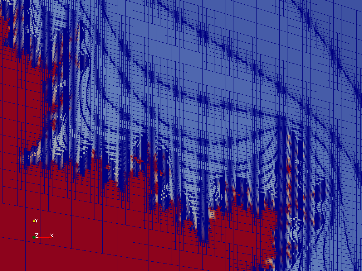
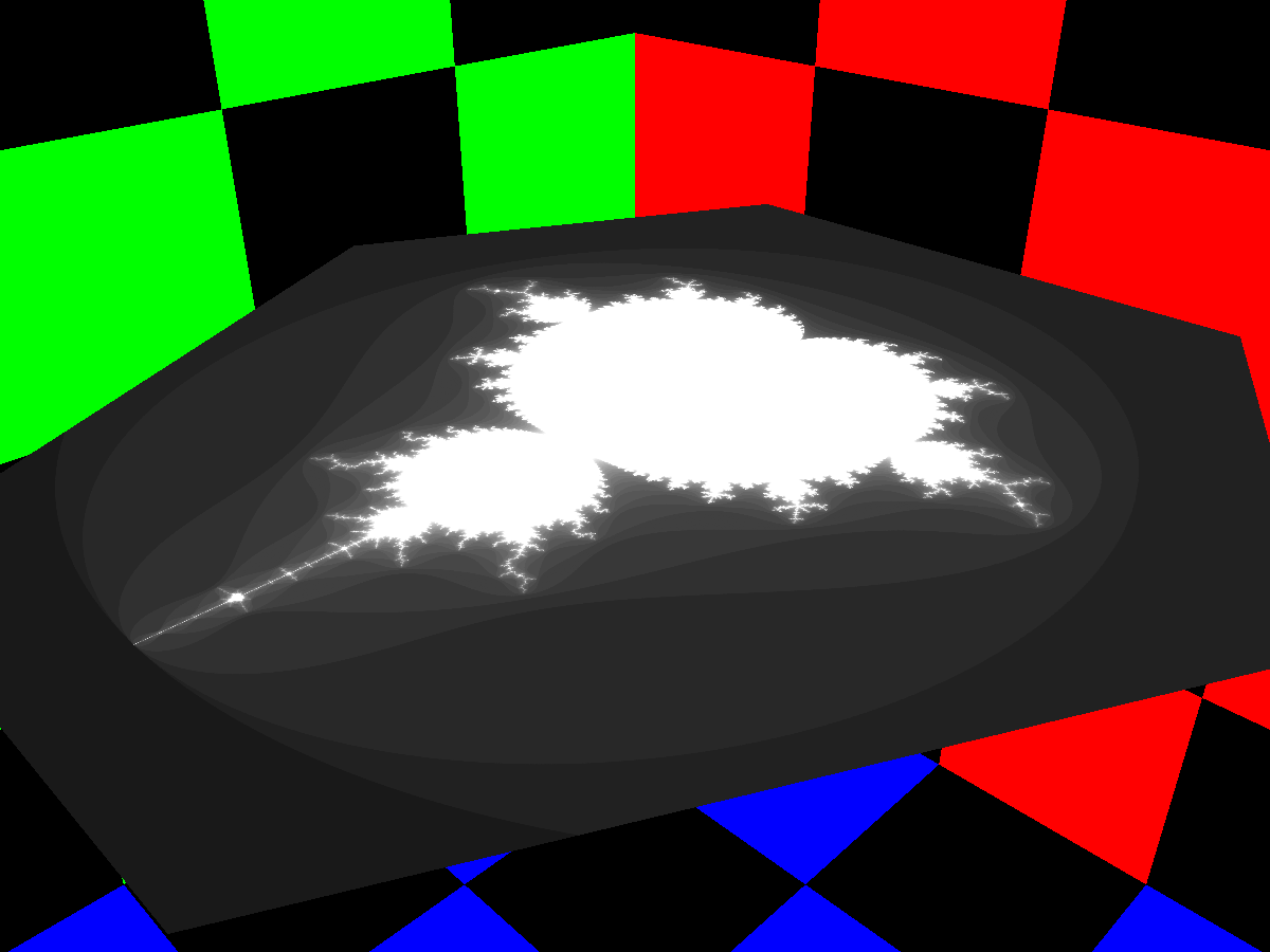
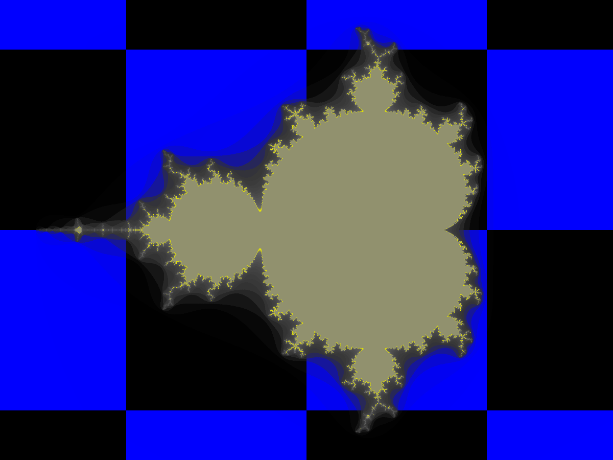
Figure 2: Rendering of the Mandelbrot set with an iteration limit of 30. The top left shows a standard visualization based on writing VTK files, showing a zoom into the adaptive 2D mesh refined to level 11. Locations drawn red have reached the iteration limit and are considered inside the set. Blue locations have values less than 1, and we see that the decrease in steps of 1/30 is reflected in the refinement pattern. Top right: One image instance computed by raycasting, using an RGB checkerboard as skybox. The manifold is rendered opaque with a color scale from grey to white. Bottom left: For the other instance we use transparency and a color model that emphasizes an iteration count just below the maximum in yellow.

4.2 Randomly distributed spheres

Our 3D example is set in a cube that we populate with spheres of random position and diameter. Again, we aim at a scale-invariant design that we realize by prescribing the probability density $\rho(s)$ of the sphere’s cross section $s$. When the spheres get smaller, we want to have more of them to give them the same optical density, which lets us choose $\rho(s)=1/s$. If we choose a minimum $s_{0}$ and maximum $s_{1}$, the expected cross section $E$ is available in closed form.

We begin with a uniformly refined mesh as before and let each process iterate through the local elements. Dividing the cross section of the element $C$ by $E$ gives us the number of spheres we would expect in this element. Running a Poisson sampler with mean $\lambda=C/E$ gives us the number of spheres to create in the element. For each of the spheres to create, we sample the radius according to $\rho$ and choose its center coordinates randomly inside the element. We implemented the samplers based on excellent material [Press et al. (1999)].— We allow for spheres that extend out of the element or out of the unit cube, and spheres that overlap with other spheres.

We focus the boundary of the spheres using a fairly sharp transfer function. The adaptation cycles proceed by refining any element that intersects any sphere’s shell between the radii $[1-\varepsilon,1+\varepsilon]r$, except when the element is already smaller than $\varepsilon r/2$. Since a shell generally touches multiple elements on remote processes, the partition traversal p4est_search_partition proves valuable again. We skip the details of repartitioning and communicating the sphere data to all relevant elements. Essentially, we ensure that any process only stores spheres whose shell intersects its elements, and that the number of element/sphere checks stays optimal. In this example, the mesh is not 2:1 balanced.

We illustrate the effect of adaptive meshing and adaptive integration in Figure 3. If the refinement is not sufficiently deep to resolve the spheres, the ray integration does not sample the shells densely enough. If we refine more deeply and choose a smaller threshold $c_{\mathrm{RK}}$, the artefacts disappear.

    

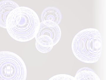
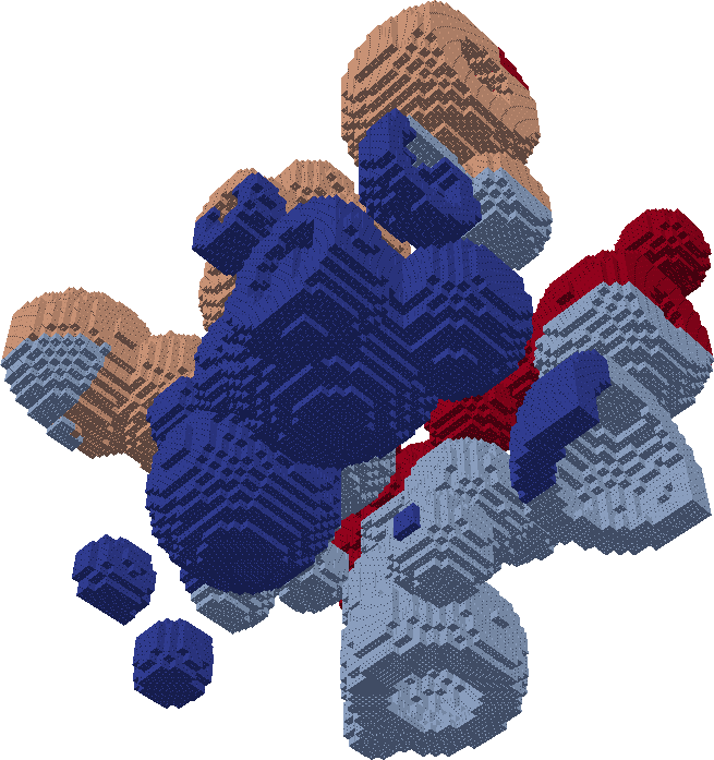
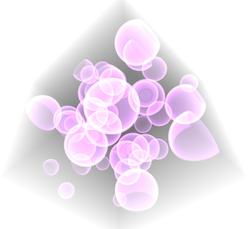
Figure 3: Top row: adaptive mesh to maximum level 4 (left) and 5 (right); rays integrated with Simpson’s rule and threshold $c_{\mathrm{RK}}=1$. We observe aliasing due to insufficient refinement and undersampling. Bottom row: setup with 44 spheres refined to level 7. Left: VTK plot of the level 7 elements partitioned on 4 processes (color coded). Right: high-accuracy rendering using the implicit Gauß method and $c_{\mathrm{RK}}=.02$.

5 Conclusion

The author would like to thank Lucas C. Wilcox for suggesting to look at Chebfun’s bivariate root finding algorithms and A. Kraut for her feedback on Poisson distributions. We would also like to thank Tobin Isaac for co-maintaining and extending the p4est software.

All p4est algorithms used in this paper are available from its public software repository [Burstedde (2010)]. We will make the building blocks of the visualization code, in particular the adaptive tree structure for storing rectangles of ray segments, available after modularizing it out of our example code. This may, however, take some time.

Appendix A Mathematical details and procedures

A.1 Computing the intersection of a ray with a tensor-product surface

For any ray vector $\vec{\mathbf{r}}$ we can construct two vectors to form the orthogonal system $(\vec{\mathbf{r}},\vec{\mathbf{d}}_{1}$, $\vec{\mathbf{d}}_{2})$. We use them to project the three coordinate equations for the intersection of the ray with a parameterized surface, written in unknowns $(\alpha,t_{1},t_{2})$ as

$$\mathbf{o}+\alpha\vec{\mathbf{r}}=\mathbf{J}_{k}(t_{1},t_{2})=\sum_{m_{1},m_{2}=0}^{R}\mathbf{Z}_{k;m_{1},m_{2}}\psi_{m_{1}}(t_{1})\psi_{m_{2}}(t_{2}),$$ (A.1)

into two equations in $(t_{1},t_{2})$,

$$0=\sum_{m_{1},m_{2}=0}^{R}P_{j;m_{1},m_{2}}\psi_{m_{1}}(t_{1})\psi_{m_{2}}(t_{2}),\quad j=1,2,$$ (A.2)

where $P_{j;m_{1},m_{2}}=\vec{\mathbf{d}}_{j}\cdot\mathbf{Z}_{k;m_{1},m_{2}}$. We can think of this as two polynomial equations in $t_{1}$ with coefficients in $t_{2}$, of which we have to find all common zeros $t_{1,i}$. Once we achieve this, we can insert each zero back into the system and solve for common zeros in the second variable.

The detailed procedure is known in commutative algebra as the resultant method (cite this). Any common zero implies a common linear factor in the two polynomials, and the conditions for the existence of such a factor can be formulated in terms of a matrix determinant. A bilinear face parameterization yields at most two intersection points, which can be computed by solving quadratic equations. A biquadratic parameterization yields at most eight intersections, which requires numeric root finding by bisection and/or Newton’s method, combined with successive division by linear factors.

A.2 Computing bounding boxes for tensor product polynomials

Given a bilinear or trilinear geometry parameterized by Lobatto points (using $\xi_{j}=j$, $j=0,1$, and $N=1$ in (2.2), (2.3)), the transformation from the reference element into space is a convex combination of the corner points. Thus, the bounding box is computed by a component-wise minimization and maximization of these points.

For higher order geometries we can reduce the three-dimensional case to considering each face in turn, at the core requiring to compute the bounding box of a two-dimensional parameterized surface. Maxima and minima can either occur at the corner points, along each edge, or inside the surface area. Corners are taken into account as is, by the same reasoning as above. Extrema along an edge can be identified by performing one-dimensional root finding of the derivative with respect to the edge coordinate. The extrema inside the surface can be found by taking the derivatives of the parameterization and performing the bivariate root finding procedure described in Section A.1. In fact, much of the mathematics and the code can be reused.

Month 2018Month 2018

References

- [1]
- Burstedde (2010) Carsten Burstedde. 2010. p4est: Parallel AMR on Forests of Octrees. (2010). http://www.p4est.org/ (last accessed September 3rd, 2018).
- Burstedde (2018) Carsten Burstedde. 2018. Parallel tree algorithms for AMR and non-standard data access. (2018). http://arxiv.org/abs/1803.08432.
- Burstedde and Holke (2017) Carsten Burstedde and Johannes Holke. 2017. Coarse mesh partitioning for tree-based AMR. SIAM Journal on Scientific Computing 39, 5 (2017), C364–C392. https://doi.org/10.1137/16M1103518
- Isaac et al. (2015) Tobin Isaac, Carsten Burstedde, Lucas C. Wilcox, and Omar Ghattas. 2015. Recursive algorithms for distributed forests of octrees. SIAM Journal on Scientific Computing 37, 5 (2015), C497–C531. DOI:http://dx.doi.org/10.1137/140970963
- Murray and vanRyper (1996) James D. Murray and William vanRyper. 1996. Encyclopedia of Graphics File Formats (second ed.). O’Reilly.
- Press et al. (1999) William H. Press, Saul A. Teukolsky, William T. Vetterling, and Brian P. Flannery. 1999. Numerical Recipes in C (second ed.). Cambridge University Press.