Compositional Stochastic Average Gradient for
Machine Learning and Related Applications

Abstract

Many machine learning, statistical inference, and portfolio optimization problems require minimization of a composition of expected value functions (CEVF). Of particular interest is the finite-sum versions of such compositional optimization problems (FS-CEVF). Compositional stochastic variance reduced gradient (C-SVRG) methods that combine stochastic compositional gradient descent (SCGD) and stochastic variance reduced gradient descent (SVRG) methods are the state-of-the-art methods for FS-CEVF problems. We introduce compositional stochastic average gradient descent (C-SAG) a novel extension of the stochastic average gradient method (SAG) to minimize composition of finite-sum functions. C-SAG, like SAG, estimates gradient by incorporating memory of previous gradient information. We present theoretical analyses of C-SAG which show that C-SAG, like SAG, and C-SVRG, achieves a linear convergence rate when the objective function is strongly convex; However, C-CAG achieves lower oracle query complexity per iteration than C-SVRG. Finally, we present results of experiments showing that C-SAG converges substantially faster than full gradient (FG), as well as C-SVRG.

Note to the readers: The short version of this paper has been accepted by the 19th International Conference on Intelligent Data Engineering and Automated Learning, 2018. This version includes detailed proofs of the main theorem and the supporting lemmas that are not included in the conference publication due to space constraints.

1 Introduction

Many problems in machine learning and statistical inference (e.g., [11]), risk management (e.g., [13]), multi-stage stochastic programming (e.g., [40]) and adaptive simulation (e.g., [17]) require minimization of linear or non-linear compositions of expected value functions (CEVF) [47]. Of particular interest are finite-sum versions of the CEVF optimization problems (FS-CEVF for short) which find applications in estimating sparse additive models (SpAM) [33], maximizing softmax likelihood functions [15] (with a wide range of applications in supervised learning [4, 16, 44]), portfolio optimization [27], and policy evaluation in reinforcement learning [41].

Stochastic gradient descent (SGD) methods [22, 35], fast first-order methods for optimization of differentiable convex functions, and their variants, have long found applications in machine learning and related areas [37, 26, 12, 6, 1, 5, 3, 23, 42, 51, 36, 52, 10, 24, 43, 32, 25, 7]. SGD methods continue to be an area of active research focused on methods for their parallelization [52, 34, 53, 21, 19, 48, 38, 54], and theoretical guarantees [32, 39, 30, 31, 20].

CEVF and FS-CEVF optimization problems have been topics of focus in several recent papers. Because SGD methods update the parameter iteratively by using unbiased samples (queries) of the gradient, the linearity of the objective function in the sampling probabilities is crucial for establishing the attractive properties of SGD. Because the CEVF objective functions violate the required linearity property, classical SGD methods no longer suffice [47]. Against this background, Wang et al. [47], introduced a class of stochastic compositional gradient descent (SCGD) algorithms for solving CEVF optimization problems. SCGD, a compositional version of stochastic quasi-gradient methods [14], has been proven to achieve convergence rate that is sub-linear in $K$, the number of stochastic samples (i.e. iterations)[47, 48, 46].

Lian et al. [27] proposed compositional variance-reduced gradient methods (C-SVRG) for FS-CEVF optimization problems. C-SVRG methods combine SCGD methods for CEVF optimization [47] with stochastic variance-reduced gradient (SVRG) method [21] to achieve a convergence rate that is constant linear in $K$, the number of stochastic samples, when the FS-CEVF to be optimized is strongly convex [27]. Recently, several extensions and variants of the C-SVRG method have been proposed. Liu et al. [29] investigated compositional variants of SVRG methods that can handle non-convex compositions of objective functions that include inner and outer finite-sum functions. Yu et al. [49] incorporated the alternating direction method of multipliers (ADMM) method [8] into C-SVRG to obtain com-SVR-ADMM to accommodate compositional objective functions with linear constraints. They also showed that com-SVR-ADMM has a linear convergence rate when the compositional objective function is strongly convex and Lipschitz smooth. Others [18, 28] have incorporated proximal gradient descent techniques into C-SVRG to handle objective functions that include a non-smooth convex regularization penalty. Despite the differences in motivations behind the various extensions of C-SVRG and their mathematical formulations, the query complexity per iteration of gradient-based update remains unchanged from that of C-SVRG. Specifically, C-SVRG methods make two oracle queries for every targeted component function to estimate gradient per update iteration.

In light of the preceding observations, it is tempting to consider compositional extensions of stochastic average gradient (SAG) [38, 36] which offers an attractive alternative to SVRG. SAG achieves $O(1/K)$ convergence rate when the objective function is convex and a linear convergence rate when the objective function is strongly-convex [36, 38]. While in the general setting, the memory requirement of SAG is $O(np)$ where $n$ is the number of data samples and $p$ is the dimensionality of the space, in many cases, it can be reduced to $O(n)$ by exploiting problem structure [38]. We introduce the compositional stochastic average gradient (C-SAG) method to minimize composition of finite-sum functions. C-SAG is a natural extension of SAG to the compositional setting. Like SAG, C-SAG estimates gradient by incorporating memory of previous gradient information. We present theoretical analyses of C-SAG which show that C-SAG, like SAG, and C-SVRG, achieves a linear convergence rate when the objective function is strongly convex. However, C-SAG achieves lower oracle query complexity per iteration than C-SVRG. We present results of experiments showing that C-SAG converges substantially faster than full gradient (FG), as well as C-SVRG.

The rest of the paper is organized as follows. Section 2 introduces the FS-CEVF optimization problem with illustrative examples. Section 3 describes the proposed C-SAG algorithm. Section 4 establishes the convergence rate of C-SAG. Section 5 presents results of experiments that compare C-SAG with C-SVRG. Section 6 concludes with a summary and discussion.

2 Finite-Sum Composition of Expected Values Optimization

In this section, we introduce some of the key definitions and illustrate how some machine learning problems naturally lead to FS-CEVF optimization problems.

2.1 Problem Formulation

A finite-sum composition of expected value function (FS-CEVF) optimization problem [27] takes the form:

$$\min_{x}f(x):=F\circ G(x)=F(G(x))$$ (1)

$$G(x)=\frac{1}{m}\sum_{j=1}^{m}G_{j}(x),\hskip 2.84544pt\hskip 2.84544ptF(y)=\frac{1}{n}\sum_{i=1}^{n}F_{i}(y).$$

where the inner function, $G:\mathbb{R}^{p}\rightarrow\mathbb{R}^{q}$, is the empirical mean of $m$ component functions, $G_{j}:\mathbb{R}^{p}\rightarrow\mathbb{R}^{q}$, and the outer function, $F:\mathbb{R}^{q}\rightarrow\mathbb{R}$, is the empirical mean of $n$ component functions, $F_{i}:\mathbb{R}^{q}\rightarrow\mathbb{R}$.

2.2 Example: Statistical Learning

Estimation of sparse additive models (SpAM) [33] is an important statistical learning problem. Suppose we are given a collection of $d$-dimensional input vectors $x_{i}=\left(x_{i1},x_{i2},\ldots,x_{i,d}\right)^{T}\in\mathbb{R}^{d}$, and associated responses $y_{i}$. Suppose that $y_{i}=\alpha+\sum_{j=1}^{d}h_{j}(x_{ij})+\epsilon_{i}$ for each pair $\left(x_{i},y_{i}\right)$. In the equation, $h_{j}:\mathbb{R}\rightarrow\mathbb{R}$ is a feature extractor and $\epsilon_{i}$ is zero-mean noise. It is customary to set $\alpha$ to zero by first subtracting from each data sample, the mean of the data samples. The feature extractors $h_{j}$ can in general be non-linear functions. SpAM estimates the feature extractor functions by solving the following minimization problem:

$$\min_{h_{j}\in\mathbb{H}_{j},j=1,\ldots,d}\frac{1}{n}\sum_{i=1}^{n}\left(y_{i}-\sum_{j=1}^{d}h_{j}(x_{i})\right)^{2},$$

where $\mathbb{H}_{j}$ is a pre-defined set of functions chosen to ensure that the model is identifiable. In many machine learning applications, the feasible sets $\mathbb{H}_{j}$ are usually compact and the feature functions $h_{j}$’s are continuously differentiable. In such scenario, it is straightforward to formulate the objective function in the form of Eq.(1).

In many practical applications of machine learning, $h_{j}$’s are assumed to be linear. In this case, the model is simplified to $y_{i}=w^{T}x_{i}+\epsilon_{i}$, where $w$ is a coefficient vector. Penalized variants of regression models (e.g. [2], [45], [50]) are often preferred to enhance stability and to induce sparse solutions. Of particular interest is the $l_{1}$-penalized regression, which is well-known by the LASSO estimator [45] which can be written as follows:

$$w^{*}=arg\min_{w}\frac{1}{n}\sum_{i=1}^{n}\left(y_{i}-w^{T}x_{i}\right)^{2}+\lambda\|w\|_{1}.$$

The objective function can be formulated as an FS-CEVF problem in Eq.(1):

$$G_{j}(w)=\left(\lambda|w_{j}|,w_{j}\cdot x_{ij}\right)^{T}\in\mathbb{R}^{2}$$

$$z=\frac{1}{d}\sum_{j=1}^{d}G_{j}(w)=\left(\frac{\lambda}{d}\|w\|_{1},\frac{1}{d}w^{T}x_{i}\right)^{T}\in\mathbb{R}^{2}$$

$$F_{i}(z)=\left(y_{i}-d\cdot z_{2}\right)^{2}+d\cdot z_{1}$$

$$\Rightarrow\hskip 2.84544pt f:=\frac{1}{n}\sum_{i=1}^{n}F_{i}\left(\frac{1}{d}\sum_{j=1}^{d}G_{j}(w)\right)=\frac{1}{n}\sum_{i=1}^{n}\left(y_{i}-w^{T}x_{i}\right)^{2}+\lambda\|w\|_{1},$$

where $z_{i}$ denotes the $i$-th element in vector $z$.

2.3 Example: Reinforcement Learning

Policy evaluation in reinforcement learning [41] presents an instance of FS-CEVF optimization. Let $S$ be a set of states, $A$ a set of actions, $\pi$: $S\rightarrow A$ a policy that maps states into actions, and $r:S\times A\rightarrow\mathbb{R}$ a reward function, Bellman equation for the value of executing policy $\pi$ starting in some state $s\in S$ is given by:

$$V^{\pi}(s)=\mathbb{E}_{\pi}\left\{r_{s,s^{\prime}}+\gamma V^{\pi}(s^{\prime})|s\right\},\forall s,s^{\prime}\in S,$$

where $r_{s,s^{\prime}}$ denotes the reward received upon transitioning from $s$ to $s^{\prime}$, and $0\leq\gamma<1$ is a discounting factor. The goal of reinforcement learning is to find an optimal policy $\pi^{\star}$ that maximizes $V^{\pi}(s)$ $\forall s\in S$.

The Bellman equation becomes intractable for moderately large $S$. Hence, in practice it is often useful to approximate $V^{\pi}(s)$ by a suitable parameterized function. For example, $V^{\pi}(s)\approx\phi_{s}^{T}w$ for some $w\in\mathbb{R}^{d}$, where $\phi_{s}\in\mathbb{R}^{d}$ is a $d$-dimensional compact representation of $s$. In this case, reinforcement learning reduces to finding an optimal $w^{*}$:

$$w^{*}=arg\min_{w}\frac{1}{|S|}\sum_{s}\left(\phi_{s}^{T}w-q_{\pi,s^{\prime}}(w)\right)^{2},$$

where $q_{\pi,s^{\prime}}(w)=\sum_{s^{\prime}}P^{\pi}_{ss^{\prime}}\left(r_{s,s^{\prime}}+\gamma\phi_{s^{\prime}}^{T}w\right)$, $P^{\pi}_{ss^{\prime}}$ is the state transition probability from $s$ to $s^{\prime}$. The objective can be formulated as an FS-CEVF problem in Eq.(1):

$$G_{j}(w)=\left(w,P^{\pi}_{sj}\left(r_{s,j}+\gamma\phi_{j}^{T}w\right)\right)^{T}\in\mathbb{R}^{d+1}$$

$$z=\frac{1}{|S|}\sum_{j=1}^{|S|}G_{j}(w)=\left(w,\frac{1}{|S|}\sum_{j=1}^{|S|}P^{\pi}_{sj}\left(r_{s,j}+\gamma\phi_{j}^{T}w\right)\right)^{T}\in\mathbb{R}^{d+1}$$

$$F_{i}(z)=\left(\phi_{i}^{T}z_{1:d}-|S|\cdot z_{d+1}\right)^{2}$$

$$\Rightarrow\hskip 2.84544pt f:=\frac{1}{|S|}\sum_{i=1}^{|S|}F_{i}\left(\frac{1}{|S|}\sum_{j=1}^{|S|}G_{j}(w)\right)=\frac{1}{|S|}\sum_{i=1}^{|S|}\left(\phi_{i}^{T}w-q_{\pi,s^{\prime}}(w)\right)^{2}.$$

2.4 Example: Mean-Variance Portfolio Optimization

Portfolio optimization characterizes human investment behavior. For each investor, the goal is to maximize the overall return on investment while minimizing the investment risk. Given $N$ assets, the objective function for the mean-variance portfolio optimization problem can be specified as:

$$\max_{x}\frac{1}{n}\sum_{i=1}^{n}<r_{i},x>-\frac{1}{n}\sum_{i=1}^{n}\left(<r_{i},x>-\frac{1}{n}\sum_{j=1}^{n}<r_{j},x>\right)^{2},$$ (2)

where $r_{i}\in R^{N}$ is the reward vector observed at time point $i$, where $i$ ranges from $1,2,...,n$. The investment vector $x$ has dimensionality $R^{N}$ and is the amount invested in each asset. To this end, overall profit is described as the mean value of the inner product of the investment vector and the observed reward vectors. The variance of the return is used as a measure of risk. To this end, overall profit is described as the mean value of the inner product of the investment vector and the observed reward vectors. The variance of the return is used as a measure of risk.

The objective can be formulated as an instance of FS-CEVF optimization problem. First, we change the sign of the maximization problem and turn it into a minimization problem. Next, specify the function $G_{j}(x)$ as:

$$G_{j}(x)=\left(\begin{tabular}[]{c}$x$\\ $<r_{j},x>$\end{tabular}\right)\in\mathbb{R}^{N+1}\textnormal{, }j=1,\ldots,n.$$ (3)

The output is a vector in $R^{N+1}$, where the investments are encoded by first $N$ dimensions and the inner product of the investment vector and the reward vector at time point $j$ is stored in the $(N+1)$-th dimension. Setting $y=\frac{1}{m}\sum_{j=1}^{m}G_{j}(x)$, we specify the function $F_{i}(y)$ as

$$F_{i}(y)=-y_{N+1}+\left(<r_{i},y_{1:N}>-y_{N+1}\right)^{2}\in\mathbb{R}\textnormal{, }i=1,\ldots,n.$$ (4)

In the equation, $y_{N+1}$ indicates the value of the $(N+1)$-th component of the vector $y$, and $y_{1:N}$ refers to the first to the $N$-th element of the vector $y$.

3 Compositional Stochastic Average Gradient Method

In this section, we describe the proposed compositional stochastic average gradient (C-SAG) method for optimizing FS-CEVF objective functions.

3.1 Stochastic average gradient algorithm

Because compositional stochastic average gradient (C-SAG) algorithm is an extension of the stochastic average gradient method (SAG) [36, 38], we begin by briefly reviewing SAG. SAG designed to optimize the sum of a finite number of smooth optimization functions:

$$\min_{x}f(x)=\frac{1}{n}\sum_{i=1}^{n}F_{i}(x)$$ (5)

The SAG iterations take the form

$$x^{k}=x^{k-1}-\frac{\alpha_{k}}{n}\sum_{i=1}^{n}y_{i}^{k},$$ (6)

where $\alpha_{k}$ is the learning rate and a random index $i_{k}$ is selected at each iteration during which we set

$$y_{i}^{k}=\begin{aligned} \begin{cases}F_{i}^{\prime}(x^{k-1})&\textnormal{if }i=i_{k}\\ y_{i}^{k-1}&\textnormal{otherwise.}\end{cases}\end{aligned}$$ (7)

Essentially, SAG maintains in memory, the gradient with respect to each function in the sum of functions being optimized. At each iteration, the gradient value of only one such function is computed and updated in memory. The SAG method estimates the overall gradient at each iteration by averaging the gradient values stored in memory. Like stochastic gradient (SG) methods [22, 35], the cost of each iteration is independent of the number of functions in the sum. However, SAG has improved convergence rate compared to conventional SG methods, from $O(1/\sqrt[]{K})$ to $O(1/K)$ in general, and from the sub-linear $O(1/K)$ to a linear convergence rate of the form $O(\rho^{K})$ for $\rho<1$ when the objective function in Eq.(5) is strongly-convex.

3.2 From SAG to C-SAG

C-SAG extends SAG to accommodate a finite-sum compositional objective function. Specifically, C-SAG maintains in memory, the items needed for updating the parameter $x^{k-1}$ to $x^{k}$. At each iteration, the relevant indices are randomly selected and the relevant gradients are computed and updated in the memory.

3.2.1 Notations

We denote by $z_{i}$ the $i$-th component of vector $z$. We denote the value of the parameter $x$ at the $k$-th iteration by $x^{k}$. Given a smooth function $H(x):\mathbb{R}^{N}\rightarrow\mathbb{R}^{M}$, $\partial H$ denotes the Jacobian of $H$ defined as:

$$\partial H:=\frac{\partial H}{\partial x}=\left(\begin{tabular}[]{c c c}$\frac{\partial[H]_{1}}{\partial[x]_{1}}$&$\cdots$&$\frac{\partial[H]_{1}}{\partial[x]_{N}}$\\ $\vdots$&$\ddots$&$\vdots$\\ $\frac{\partial[H]_{M}}{\partial[x]_{1}}$&$\cdots$&$\frac{\partial[H]_{M}}{\partial[x]_{N}}$\end{tabular}\right).$$

The value of the Jacobian evaluated at $x_{k}$ is denoted by $\partial H(x_{k})$. For function $h:\mathbb{R}^{N}\rightarrow\mathbb{R}$, the gradient of $h$ is defined by

$$\nabla h(x) =\left(\frac{\partial h(x)}{\partial x}\right)^{T}$$

$$=\left(\frac{\partial h}{\partial[x]_{1}},\cdots,\frac{\partial h}{\partial[x]_{N}}\right)^{T}$$

The gradient of a composition function $f=F(G(x))$ is given by chain rule:

$$\nabla f(x)=\left(\partial G(x)\right)^{T}\nabla F(G(x)),$$ (8)

where $\nabla F(G(x))$ stands for the gradient of $F$ evaluated at $G(x)$. Evaluating the gradient requires three key terms, namely, the Jacobian of the inner function $\partial G(\cdot)$, value of the inner function $G(\cdot)$, and the gradient of the outer function $\nabla F(\cdot)$.

We use $\hat{f}$ to denote an estimate of the function $f$, and analogously, $\partial\hat{H}$ and $\nabla\hat{h}(x)$ to denote estimates of Jacobian matrices $\partial H$ and gradient vectors $\nabla h(x)$ respectively. To minimize notational clutter, we use $G_{j}^{k}$ to denote $G_{j}(x^{k})$, $\partial G_{j}^{k}$ to denote $\partial G_{j}(x^{k})$, and $\nabla F_{i}^{k}$ to denote $\nabla F_{i}(x^{k})$. Given a set $A$, we use $|A|$ to denote the number of elements in the set. We use $\mathbb{E}$ to denote expectation.

3.2.2 C-SAG Algorithm

We define memories $J_{j}$ for storing the Jacobian of the inner function $\partial G_{j}(\cdot)$, $V_{j}$ for storing the value of the inner function $G_{j}(\cdot)$, and $Q_{i}$ for storing the gradient of the outer function $\nabla F_{i}(\cdot)$. At iteration $k$, we randomly select indices $j_{k}$, $i_{k}$, and a mini-batch $A_{k}$. We update the $J_{j}$’s as follows:

$$J_{j}^{k}=\begin{aligned} \begin{cases}\partial G_{j}(x^{k-1})&\textnormal{if }j=j_{k}\\ J_{j}^{k-1}&\textnormal{otherwise.}\end{cases}\end{aligned}$$ (9)

We update the $V_{j}$’s as follows:

$$V_{j}^{k}=\begin{aligned} \begin{cases}G_{j}(x^{k-1})&\textnormal{if }j\in A_{k}\\ V_{j}^{k-1}&\textnormal{otherwise.}\end{cases}\end{aligned}$$ (10)

We update the $Q_{i}$’s as follows:

$$Q_{i}^{k}=\begin{aligned} \begin{cases}\nabla F_{i}\left(\frac{1}{m}\sum_{j=1}^{m}V_{j}^{k}\right)&\textnormal{if }i=i^{k}\\ Q_{i}^{k-1}&\textnormal{otherwise.}\end{cases}\end{aligned}$$ (11)

Finally, the update rule is obtained by substituting Eq.(9)-Eq.(11) into Eq.(8):

$$x^{k}=x^{k-1}-\alpha\nabla\hat{f}^{k}$$ (12)

$$\nabla\hat{f}^{k}=(\partial\hat{G}(x^{k-1}))^{T}\nabla\hat{F}(\hat{G}(x^{k-1}))$$

$$\partial\hat{G}(x^{k-1})=\frac{1}{m}\sum_{j=1}^{m}J_{j}^{k}$$

$$\hat{G}(x^{k-1})=\frac{1}{m}\sum_{j=1}^{m}V_{j}^{k}$$

$$\nabla\hat{F}(\hat{G}(x^{k-1}))=\frac{1}{n}\sum_{i=1}^{n}Q_{i}^{k}$$

Algorithm 1 C-SAG

1:Require: $K$ (update period), $\alpha$ (step size), $S$ (maximum number of training iterations), $a$ (mini batch size)

2:while $true$ do

3:     $\backslash\backslash$ Refresh memory, evaluate full gradient

4:     $J_{j}=\partial G_{j}(\tilde{x})$ for $j=1,...,m$ $\triangleright$ m queries

5:     $V_{j}=G_{j}(\tilde{x})$ for $j=1,...,m$ $\triangleright$ m queries

6:     $Q_{i}=\nabla F_{i}(G(\tilde{x}))$ for $i=1,...,n$ $\triangleright$ n queries

7:     $x_{0}=\tilde{x}-\alpha\nabla f(\tilde{x})$

8:     for $k=1$ to $K$ do

9:         Uniformly select $j_{k}$ from $\left[1,2,...,m\right]$, mini-batch $A_{k}$ from $\left[1,2,...,m\right]$ and $i_{k}$ from $\left[1,2,...,n\right]$

10:         $\backslash\backslash$Estimate $\nabla\hat{f}^{k}$

11:         update memory $J$ by Eq.(9) $\triangleright$ 1 query

12:         update memory $V$ by Eq.(10) $\triangleright$ $|A|$ queries

13:         update memory $Q$ by Eq.(11) $\triangleright$ 1 query

14:         estimate $\partial\hat{G}(x^{k-1})=\frac{1}{m}\sum_{j=1}^{m}J_{j}^{k}$

15:         estimate $\hat{G}(x^{k-1})=\frac{1}{m}\sum_{j=1}^{m}V_{j}^{k}$

16:         estimate $\nabla\hat{F}(\hat{G}(x^{k-1}))=\frac{1}{n}\sum_{i=1}^{n}Q_{i}^{k}$

17:         $\nabla\hat{f}^{k}=(\partial\hat{G}(x^{k-1}))^{T}\nabla\hat{F}(\hat{G}(x^{k-1}))$

18:         $x^{k}=x^{k-1}-\alpha\nabla\hat{f}^{k}$      

19:     $\tilde{x}=x^{K}$

20:     if converged or $S$ reached then

21:         return $x^{K}$      

In addition, because the gradient estimate is biased in the case of FS-CEVF objective function [27], to improve the stability of the algorithm, we use a refresh mechanism to evaluate the exact full gradient periodically and update $J$, $V$, and $Q$. The frequency of refresh is controlled by a pre-specified parameter $K$. The complete algorithm is shown in Algorithm 1.

3.3 Oracle Query Complexity of C-SAG

In the algorithm, we define the cost of an oracle query as the unit cost of computing $\partial G_{j}(\cdot)$, $G_{j}(\cdot)$, and $\nabla F_{i}(\cdot)$. Evaluating the exact full gradient, such as line 4, 5, and 6 in Algorithm 1, takes $m$, $m$, and $n$ oracle queries, for $\partial G(\cdot)$, $G(\cdot)$, and $\nabla F(\cdot)$ respectively, yielding an oracle query complexity of $O(2m+n)$. On the other hand, lines 11 to 13 of Algorithm 1 estimate gradient by incorporating the memory of previous steps, yielding $2+|A_{k}|$ queries at each iteration, which is independent of the number of component functions.

We proceed to compare the oracle query complexity per iteration between C-SAG with the state-of-the-art C-SVRG methods C-SVRG-1 and C-SVRG-2 [27]. C-SVRG-1 requires $2A+4$ oracle queries in each iteration (where $A$ is the mini-batch size used by C-SVRG-1) except for the reference update iteration, in which exact full gradient is evaluated which requires $2m+n$ queries. The reference update iteration in C-SVRG methods is equivalent corresponds to the memory refreshing mechanism in C-SAG. In addition, C-SVRG-2 takes $2A+2B+2$ queries per iteration (where $B$ is a second mini-batch size used by C-SVRG-2) except for the reference update iteration. On the other hand, the proposed C-SAG takes $A+2$ queries per iteration except for the refresh iteration. The number of queries required by C-SAG during memory refresh iterations are the same as those for C-SVRG-1 and C-SVRG-2 during their reference update iterations. We conclude that C-SAG, in general, incurs only half the oracle query complexity of C-SVRG-1, and less than half that of C-SVRG-2.

4 Convergence Analysis of C-SAG

We proceed to establish the convergence and the convergence rate of C-SAG. Because of space constraints, the details of the proof are relegated to the Appendix.

Suppose the objective function in Eq.(1) has a minimizer $x^{*}$. In what follows, we make the same assumptions regarding the functions $f(\cdot)$, $F(\cdot)$, and $G(\cdot)$ as those used in [27] to establish the convergence of C-SVRG methods. We assume:

• Strongly Convex Objective: $f(x)$ in Eq.(1) is strongly convex with parameter $\mu_{f}$:

  $$f(y)\geq f(x)+<\nabla f(x),y-x>+\frac{\mu_{f}}{2}\|y-x\|^{2},\hskip 2.84544pt\forall x,y. \Delta_{1}$$ ()

• Bounded Jacobian of Inner Functions We assume that the Jacobian of all inner component functions are upper-bounded by $B_{G}$,

  $$\|\partial G_{j}(x)\|\leq B_{G},\hskip 2.84544pt\forall x,\forall j\in\left\{1,\ldots,m\right\}. \Delta_{2}$$ ()

  Using this inequality, we can bound the estimated Jacobian $J_{j}^{k}$. Because $J_{j}^{k}=\partial G_{j}^{k^{\prime}}$ for some $k^{\prime}<k$, we have:

  $$\|J_{j}\|\leq B_{G},\hskip 2.84544pt\forall j\in\left\{1,\ldots,m\right\}. \Delta_{3}$$ ()

• Lipschitz Gradients: We assume that there is a constant $L_{F}$ such that $\forall x,\forall y,\forall i\in\left\{1,\ldots n\right\}$, the following holds:

  $$\|\nabla F_{i}(x)-\nabla F_{i}(y)\|\leq L_{F}\|x-y\|, \Delta_{4}$$ ()

Armed with the preceding assumptions, we proceed to establish the convergence of C-SAG.

Theorem 4.1

(Convergence of C-SAG algorithm). For the proposed C-SAG algorithm, we have:

$$\frac{1}{K}\sum_{k=0}^{K-1}\mathbb{E}\|x_{k}-x^{*}\|^{2}\leq\hskip 2.84544pt\frac{\gamma_{1}}{\gamma_{2}}\mathbb{E}\|\tilde{x}-x^{*}\|^{2}.$$

where

$$\gamma_{1}=\frac{1}{K}+\left(n\sigma_{1}+3m\left(1-(\frac{a}{m})^{2}\right)\sigma_{2}\right)B_{G}^{4}L_{F}^{2}$$

$$\gamma_{2}=\alpha\mu_{f}-\left(\frac{32\alpha(m-a)}{m\mu_{f}}+3a(2-\frac{a}{m})\sigma_{2}\right)B_{G}^{4}L_{F}^{2},$$

and

$$\begin{aligned} \sigma_{1}=&9\alpha^{2}\left((m-1)^{2}(1-\frac{1}{n})(n+2)+(n-1)(4m-3)\right)+16\alpha n\frac{(m-1)^{2}(1-\frac{1}{n})^{2}+(1-\frac{1}{n})^{2}}{\mu_{f}}\\ \end{aligned}$$

$$\begin{aligned} \sigma_{2}=&\frac{9\alpha^{2}}{m}\left((m-1)^{2}(2n-1)+n+4n(m-1)\right)+16\alpha\frac{(1-\frac{1}{m})^{2}m+16(m-a)}{m^{2}\mu_{f}}.\end{aligned}$$

Proof

The proof proceeds as follows: (i) We express $\mathbb{E}\|x^{k}-x^{*}\|^{2}$ in terms of $J^{k-1}$, $V^{k-1}$, $Q^{k-1}$, and $x^{k-1}$; (ii) We use the assumptions (a) through (c) above to bound $J^{k-1}$, $V^{k-1}$, and $Q^{k-1}$ in terms of $x^{k-1}$ and $\tilde{x}$; and (iii) We use the preceding bounds to establish the convergence of C-SAG, and the choice of parameters (refresh frequency $1/K$, batch size $a$, and learning rate $\alpha$ etc.) that ensure convergence (See Appendix for details)

Corollary 1

(Convergence rate of C-SAG algorithm). Suppose we choose the user-specified parameters of C-SAG such that:

$$\begin{cases}&a>m\left(1-\frac{\mu_{f}^{2}}{128B_{G}^{4}L_{F}^{2}}\right),\\ &\alpha<\min\left\{\alpha_{1},\alpha_{2},\alpha_{3}\right\},\\ &K>\frac{8}{\alpha\mu_{f}},\end{cases}$$

where

$$\alpha_{1}=\frac{m\left(\frac{\mu_{f}}{12a\left(2-\frac{a}{m}\right)B_{G}^{4}L_{F}^{2}}-16\frac{(1-\frac{1}{m})^{2}m+16(m-a)}{m^{2}\mu_{f}}\right)}{9\left((m-1)^{2}(2n-1)+n+4n(m-1)\right)}$$

$$\alpha_{2}=\frac{\frac{\mu_{f}}{8nB_{G}^{4}L_{F}^{2}}-16n\frac{(m-1)^{2}(1-\frac{1}{n})^{2}+(1-\frac{1}{n})^{2}}{\mu_{f}}}{9\left((m-1)^{2}(1-\frac{1}{n})(n+2)+(n-1)(4m-3)\right)}$$

$$\alpha_{3}=\frac{m\left(\frac{\mu_{f}}{24m\left(1-\left(\frac{a}{m}\right)^{2}\right)B_{G}^{4}L_{F}^{2}}-16\frac{(1-\frac{1}{m})^{2}m+16(m-a)}{m^{2}\mu_{f}}\right)}{9\left((m-1)^{2}(2n-1)+n+4n(m-1)\right)},$$

Then we have:

$$\frac{1}{K}\sum_{k=0}^{K-1}\mathbb{E}\|x_{k}-x^{*}\|^{2}<\frac{3}{4}\mathbb{E}\|\tilde{x}-x^{*}\|^{2}.$$

Corollary 1 implies a linear convergence rate [27].

5 Experimental evaluation of C-SAG

We report results of comparison of C-SAG with two variants of C-SVRG [27], C-SVRG-1 and C-SVRG-2, which are among the state-of-the-art methods for FS-CEVF optimization, as well as the classical full gradient (FG) method [9], on the mean-variance portfolio optimization problem (See Section 2 for details).

Our experimental setup closely follows the setup in [27]. Synthetic data were drawn from a multi-variate Gaussian distribution and absolute values of the data samples were retained. We generated two synthetic data sets (D1 and D2). D1 consists of 2000 time points, and 200 assets, i.e., $n=2000$, $N=200$; D2 consists of 5000 time points, and 300 assets, i.e., $n=5000$, $N=300$. We also controlled $\kappa_{cov}$, the condition number of the covariance matrix used in the multi-variate Gaussian distribution to generate the synthetic data. We compared our proposed algorithm to the classical FG method [9], and two state-of-the-art algorithms, C-SVRG-1 [27] and C-SVRG-2 [27]. The initialization and the step sizes were chosen to be identical for all algorithms. The parameters are set to their default values in the implementation provided by the authors of [27]: The size of the mini-batch was set to 20 ($a=20$), the update period was set to 20 iterations ($K=20$), and the constant step size was set to 0.12 ($\alpha=0.12$).

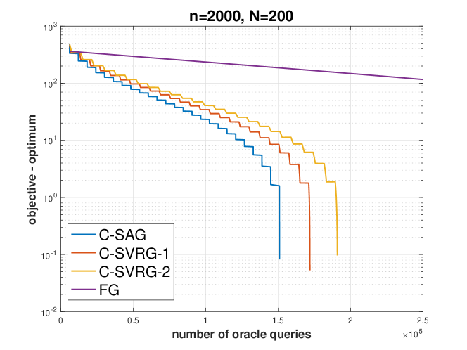
(a) $\kappa_{cov}=20$

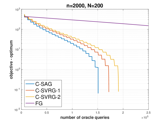
(b) $\kappa_{cov}=100$

Figure 1: Mean-variance portfolio optimization on synthetic data D1 with 200 assets ($N=300$) and the number of time points $n=2000$. The logarithm of the objective value minus the optimum is plotted along the Y-axis and the number of oracle queries is plotted along the X-axis. The $\kappa_{cov}$ is the conditional number of the covariance matrix of the corresponding Gaussian distribution used to generate reward vectors.

The experimental results comparing the different methods on data sets D1 and D2 are shown in Fig. 1 and Fig. 2 respectively. The number of oracle queries is proportional to the runtime of the algorithm. Note that the sudden drop at the tail of each curve results from treating the smallest objective value in the convergence sequence, which is usually found at the end of the sequence, as the optimum value. We observe that on both data sets, all stochastic gradient methods converge faster than full gradient (FG) method, and that C-SAG achieves better (lower) value of the objective function at each iteration. Although the three stochastic methods under comparison (C-SVRG-1, C-SVRG-2, and our method, C-SAG) all have linear convergence rates, C-SAG converges faster in practice by virtue of lower oracle query complexity per iteration as compared to C-SVRG-1 and C-SVRG-2.

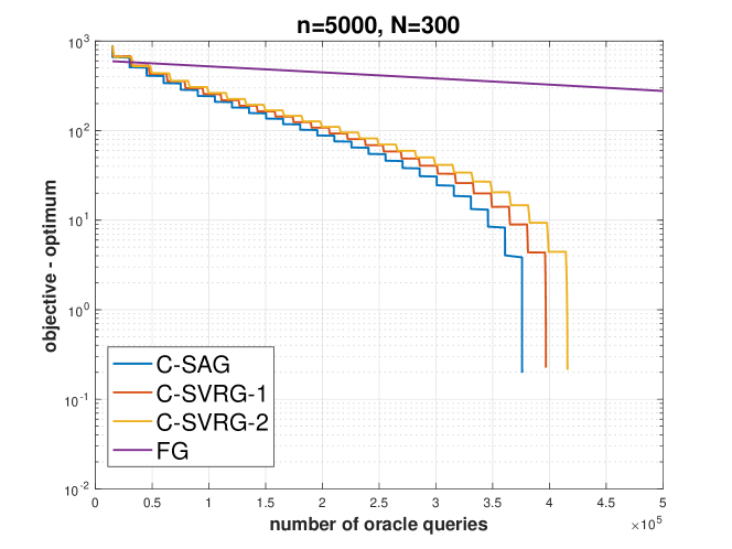
(a) $\kappa_{cov}=20$

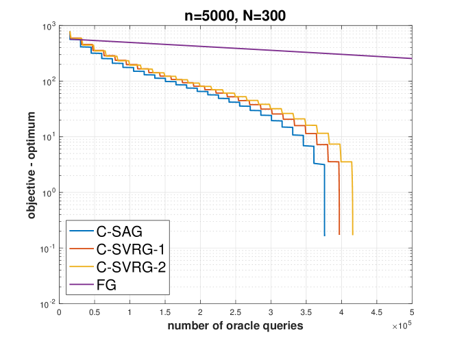
(b) $\kappa_{cov}=100$

Figure 2: Mean-variance portfolio optimization on synthetic data D2 with 300 assets ($N=200$) and the number of time points $n=5000$. The logarithm of the objective value minus the optimum is plotted along the Y-axis and the number of oracle queries is plotted along the X-axis. The $\kappa_{cov}$ is the conditional number of the covariance matrix of the corresponding Gaussian distribution used to generate reward vectors.

C-SAG has three user-specified parameters. It is especially interesting as to how the update period, $K$, and the size of the mini-batch, $a$, impact the convergence of C-SAG. The parameter $K$ controls the frequency at which the full gradient is computed, and hence represents a trade-off between the accuracy and the computational efficiency of C-SAG. We experimented with C-SAG with $K$ set to 10, 20, 50, and 200 iterations. The results of this experiment are summarized in Fig. 3(a). As expected, C-SAG converges faster for larger values of $K$ (i.e., the time elapsed between consecutive memory refresh events or full gradient computation is longer). However, for larger values of $K$, C-SAG may fail to converge to the optimum value of the objective function.

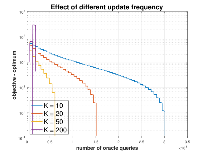
(a) Effect of different update period

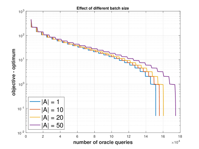
(b) Effect of different mini-batch size

Figure 3: Effect of user-specified parameters: (a) the duration between successive full gradient computations, $K$ and (b) mini-batch size, $|A|$, on the performance of C-SAG.

A second parameter of interest is the size of the mini-batch used by C-SAG. We experiment with different mini-batch sizes, from 1, 10, 20, to 50. The results are shown in Figure 3(b). Not surprisingly, we observe that C-SAG converges faster as mini-batch size is decreased.

6 Summary and Discussion

Many machine learning, statistical inference, and portfolio optimization problems require minimization of a composition of expected value functions. We have introduced C-SAG, a novel extension of SAG, to minimize composition of finite-sum functions, i.e., finite sum variants of composition of expected value functions. We have established the convergence of the resulting algorithm and shown that it, like other state-of-the-art methods e.g., C-SVRG, achieves a linear convergence rate when the objective function is strongly convex, while benefiting from lower oracle query complexity per iteration as compared to C-SVRG. We have presented results of experiments that show that C-SAG converges substantially faster than the state-of-the art C-SVRG variants.

Work in progress is aimed at (i) analyzing the convergence rate of C-SAG for general (weakly convex) problems; (ii) developing a distributed optimization algorithm for the composition finite-sum problems by combining C-SAG with the ADMM framework [8]; and (iii) applying C-SAG and its variants to problems of practical importance in machine learning.

Appendix

We present here the convergence analysis of the C-SAG algorithm.

Preliminaries

Let $x^{*}$ be the unique minimizer of the $f$ in Eq.(1). Let the random variables $z_{i}^{k}$, $y_{i}^{k}$, and $w_{i}^{k}$ be defined as follows:

$$z_{i}^{k}=\begin{cases}1-\frac{1}{m}&\hskip 14.22636pt,\textnormal{with probability}=\frac{1}{m}\\ -\frac{1}{m}&\hskip 14.22636pt,\textnormal{otherwise}\end{cases}$$ (13)

$$y_{i}^{k}=\begin{cases}1-\frac{a}{m}&\hskip 14.22636pt,\textnormal{with probability}=\frac{a}{m}\\ -\frac{a}{m}&\hskip 14.22636pt,\textnormal{otherwise}\end{cases}$$

$$w_{i}^{k}=\begin{cases}1-\frac{1}{n}&\hskip 14.22636pt,\textnormal{with probability}=\frac{1}{n}\\ -\frac{1}{n}&\hskip 14.22636pt,\textnormal{otherwise}\end{cases},$$

where $a$ is the size of the mini batch $A_{k}$. We can rewrite $J_{j}$, $V_{j}$, and $Q_{i}$ as

$$J_{j}^{k}=(1-\frac{1}{m})J_{j}^{k-1}+\frac{1}{m}\partial G_{j}^{k-1}+z_{j}^{k}\left[\partial G_{j}^{k-1}-J_{j}^{k-1}\right],$$ (14)

$$V_{j}^{k}=(1-\frac{a}{m})V_{j}^{k-1}+\frac{a}{m}G_{j}^{k-1}+y_{j}^{k}\left[G_{j}^{k-1}-V_{j}^{k-1}\right],$$

$$Q_{j}^{k}=(1-\frac{1}{n})Q_{i}^{k-1}+\frac{1}{n}\nabla F_{i}(\hat{G}^{k-1})+w_{i}^{k}\left[\nabla F_{i}(\hat{G}^{k-1})-Q_{i}^{k-1}\right],$$

and therefore Eq.(12) is equivalent to

$$x^{k} =x^{k-1}- \alpha\nabla\hat{f}(x^{k-1})$$ (15)

$$=x^{k-1}- \alpha\left(\partial\hat{G}^{k-1}\right)^{T}\left(\nabla\hat{F}(\hat{G}^{k-1}\right)$$

$$=x^{k-1}- \alpha\left(\frac{1}{m}\sum_{j=1}^{m}J_{j}^{k}\right)^{T}\left(\frac{1}{n}\sum_{i=1}^{n}Q_{i}^{k}\right)$$

$$=x^{k}- \frac{\alpha}{mn}\left((1-\frac{1}{m})e^{T}J^{k-1}+\partial G^{k-1}+(z^{k})^{T}\left[G^{\prime k-1}-J^{k-1}\right]\right)^{T}$$

$$\left((1-\frac{1}{n})e^{T}Q^{k-1}+\nabla F(\hat{G}^{k-1})+(w^{k})^{T}\left[F^{\prime}(\hat{G}^{k-1})-Q^{k-1}\right]\right)$$

$$=x^{k-1}- \frac{\alpha}{mn}S$$

with

$$e=\left(\begin{tabular}[]{c}$I$\\ $\vdots$\\ $I$\end{tabular}\right)\in\mathbb{R}^{mq\times q},\hskip 2.84544pt G^{\prime k-1}=\left(\begin{tabular}[]{c}$\partial G_{1}^{k-1}$\\ $\vdots$\\ $\partial G_{m}^{k-1}$\end{tabular}\right)\in\mathbb{R}^{mq},\hskip 2.84544pt F^{\prime k-1}=\left(\begin{tabular}[]{c}$\nabla F_{1}^{k-1}$\\ $\vdots$\\ $\nabla F_{n}^{k-1}$\end{tabular}\right)\in\mathbb{R}^{mq\times p},$$

$$J^{k-1}=\left(\begin{tabular}[]{c}$J_{1}^{k-1}$\\ $\vdots$\\ $J_{m}^{k-1}$\end{tabular}\right)\in\mathbb{R}^{mq\times p},\hskip 2.84544pt Q^{k-1}=\left(\begin{tabular}[]{c}$Q_{1}^{k-1}$\\ $\vdots$\\ $Q_{m}^{k-1}$\end{tabular}\right)\in\mathbb{R}^{mq},\hskip 2.84544pt z^{k}=\left(\begin{tabular}[]{c}$z_{1}^{k}I$\\ $\vdots$\\ $z_{m}^{k}I$\end{tabular}\right)\in\mathbb{R}^{mq\times q},$$

$$w^{k}=\left(\begin{tabular}[]{c}$w_{1}^{k}I$\\ $\vdots$\\ $w_{m}^{k}I$\end{tabular}\right)\in\mathbb{R}^{mq\times q}.$$

In the last line of Eq.(15), we denote

$$S= \left((1-\frac{1}{m})e^{T}J^{k-1}+\partial G^{k-1}+(z^{k})^{T}\left[G^{\prime k-1}-J^{k-1}\right]\right)^{T}$$

$$\left((1-\frac{1}{n})e^{T}Q^{k-1}+\nabla F(\hat{G}^{k-1})+(w^{k})^{T}\left[F^{\prime}(\hat{G}^{k-1})-Q^{k-1}\right]\right).$$

Expanding the matrix multiplication, we obtain

$$S= (1-\frac{1}{m})(1-\frac{1}{n})(J^{k-1})^{T}ee^{T}Q^{k-1}$$ (16)

$$+ (1-\frac{1}{m})(J^{k-1})^{T}e\nabla F(\hat{G}^{k-1})$$

$$+ (1-\frac{1}{m})(J^{k-1})^{T}e(w^{k})^{T}\left[F^{\prime}(\hat{G}^{k-1})-Q^{k-1}\right]$$

$$+ (1-\frac{1}{n})(\partial G^{k-1})^{T}e^{T}Q^{k-1}$$

$$+ (\partial G^{k-1})^{T}\nabla F(\hat{G}^{k-1})$$

$$+ (\partial G^{k-1})^{T}(w^{k})^{T}\left[F^{\prime}(\hat{G}^{k-1})-Q^{k-1}\right]$$

$$+ (1-\frac{1}{n})\left[G^{\prime k-1}-J^{k-1}\right]^{T}(z^{k})e^{T}Q^{k-1}$$

$$+ \left[G^{\prime k-1}-J^{k-1}\right]^{T}(z^{k})\nabla F(\hat{G}^{k-1})$$

$$+ \left[G^{\prime k-1}-J^{k-1}\right]^{T}(z^{k})(w^{k})^{T}\left[F^{\prime}(\hat{G}^{k-1})-Q^{k-1}\right].$$

In addition to the assumptions in Section 4, we make use of several inequalities in our proof. First, for any $\alpha>0$, we have:

$$\frac{1}{\alpha}\|x\|^{2}+\alpha\|y\|^{2}\geq|\left\langle x,y\right\rangle|. \Box_{1}$$ ()

Second, for any $x$ we have:

$$\|x_{1}+x_{2}+\ldots+x_{t}\|^{2}\leq t\left(\|x_{1}\|^{2}+\ldots+\|x_{t}\|^{2}\right),\hskip 2.84544pt\forall t\in\mathbb{N}^{+}. \Box_{2}$$ ()

Third, for any matrix $A$ and vector $x$, we have:

$$\|Ax\|^{2}\leq\|A\|^{2}\|x\|^{2} \Box_{3}$$ ()

Lastly, note that $\nabla f(x^{*})=(\partial G(x^{*}))^{T}\nabla F(G(x^{*}))=0$.

Proof of Convergence of C-SAG

We decompose the expectation $\mathbb{E}\|x_{k}-x^{*}\|^{2}$ as follows:

$$\mathbb{E}\|x^{k}-x^{*}\|^{2} =\mathbb{E}\|x^{k-1}-x^{*}\|^{2}+\mathbb{E}\|x^{k}-x^{k-1}\|^{2}+2\mathbb{E}\left\langle x^{k}-x^{k-1},x^{k-1}-x^{*}\right\rangle$$ (17)

$$=\mathbb{E}\|x^{k-1}-x^{*}\|^{2}+\alpha^{2}\mathbb{E}\|S\|^{2}-2\alpha\mathbb{E}\left\langle S,x^{k-1},x^{*}\right\rangle.$$

Recalling that $\mathbb{E}[z^{k}]=0$, $\mathbb{E}[w^{k}]=0$, and $z^{k}$, $w^{k}$ are independent, we can rewrite the last term as:

$$\mathbb{E}\left\langle S,x^{k-1},x^{*}\right\rangle = (1-\frac{1}{m})(1-\frac{1}{n})\left\langle(J^{k-1})^{T}ee^{T}Q^{k-1},x^{k-1}-x^{*}\right\rangle s_{1}$$ ()

$$+ (1-\frac{1}{m})\left\langle(J^{k-1})^{T}e\nabla F(\hat{G}^{k-1}),x^{k-1}-x^{*}\right\rangle s_{2}$$ ()

$$+ (1-\frac{1}{n})\left\langle(\partial G^{k-1})^{T}e^{T}Q^{k-1},x^{k-1}-x^{*}\right\rangle s_{3}$$ ()

$$+ \left\langle(\partial G^{k-1})^{T}\nabla F(\hat{G}^{k-1}),x^{k-1}-x^{*}\right\rangle. s_{4}$$ ()

Letting $\beta_{1}=(1-\frac{1}{m})(1-\frac{1}{n})$ we have:

$$s_{1} =(1-\frac{1}{m})(1-\frac{1}{n})\left\langle(J^{k-1})^{T}ee^{T}Q^{k-1},x^{k-1}-x^{*}\right\rangle$$ (18)

$$\overset{\Box_{1}}{\geq}-\frac{\beta_{1}}{\alpha_{1}}\|(J^{k-1})^{T}ee^{T}Q^{k-1}\|^{2}-\alpha_{1}\beta_{1}\|x^{k-1}-x^{*}\|^{2}$$

$$\overset{\Box_{3}}{\geq}-\frac{\beta_{1}}{\alpha_{1}}\|e^{T}J^{k-1}\|^{2}\|e^{T}Q^{k-1}\|^{2}-\alpha_{1}\beta_{1}\|x^{k-1}-x^{*}\|^{2}$$

$$=-\frac{\beta_{1}}{\alpha_{1}}\|\sum_{j=1}^{m}J_{j}^{k-1}\|^{2}\|\sum_{i=1}^{n}Q_{i}^{k-1}-\nabla F_{i}(G^{*})\|^{2}-\alpha_{1}\beta_{1}\|x^{k-1}-x^{*}\|^{2}$$

$$\overset{\overset{\Box_{2}}{\Delta_{3}}}{\geq}-\frac{\beta_{1}}{\alpha_{1}}m^{2}B_{G}^{2}n\underset{T_{0}}{\underbrace{\sum_{i=1}^{n}\|Q_{i}^{k-1}-\nabla F_{i}(G^{*})\|^{2}}}-\alpha_{1}\beta_{1}\|x^{k-1}-x^{*}\|^{2},$$

for any $\alpha_{1}>0$. Letting $\beta_{2}=1-\frac{1}{m}$, we have:

$$s_{2} =(1-\frac{1}{m})\left\langle(J^{k-1})^{T}e\nabla F(\hat{G}^{k-1}),x^{k-1}-x^{*}\right\rangle$$ (19)

$$\overset{\Box_{1}}{\geq}-\frac{\beta_{2}}{\alpha_{2}}\|(J^{k-1})^{T}e\nabla F(\hat{G}^{k-1})\|^{2}-\alpha_{2}\beta_{2}\|x^{k-1}-x^{*}\|^{2}$$

$$\overset{\Box 3}{\geq}-\frac{\beta_{2}}{\alpha_{2}}\|e^{T}J^{k-1}\|^{2}\|\nabla F(\hat{G}^{k-1})-\nabla F(G^{*})\|^{2}-\alpha_{2}\beta_{2}\|x^{k-1}-x^{*}\|^{2}$$

$$\overset{\Delta_{4}}{\geq}-\frac{\beta_{2}}{\alpha_{2}}B_{G}^{2}L_{F}^{2}\|\hat{G}^{k-1}-G^{*}\|^{2}-\alpha_{2}\beta_{2}\|x^{k-1}-x^{*}\|^{2}$$

$$\geq-\frac{\beta_{2}}{\alpha_{2}}\frac{B_{G}^{2}L_{F}^{2}}{m}\underset{T_{1}}{\underbrace{\sum_{j=1}^{m}\|V_{j}^{k}-G_{j}^{*}\|^{2}}}-\alpha_{2}\beta_{2}\|x^{k-1}-x^{*}\|^{2}$$

for any $\alpha_{2}>0$. Similarly letting $\beta_{3}=1-\frac{1}{n}$, we have:

$$s_{3} =(1-\frac{1}{n})\left\langle(\partial G^{k-1})^{T}e^{T}Q^{k-1},x^{k-1}-x^{*}\right\rangle$$ (20)

$$\overset{\Box_{1}}{\geq}-\frac{\beta_{3}}{\alpha_{3}}\|(\partial G^{k-1})^{T}e^{T}Q^{k-1})\|^{2}-\alpha_{3}\beta_{3}\|x^{k-1}-x^{*}\|^{2}$$

$$\overset{\Box_{3}}{\geq}-\frac{\beta_{3}}{\alpha_{3}}\|\partial G^{k-1})\|^{2}\|e^{T}Q^{k-1}\|^{2}-\alpha_{3}\beta_{3}\|x^{k-1}-x^{*}\|^{2}$$

$$=-\frac{\beta_{3}}{\alpha_{3}}\|\partial G^{k-1})\|^{2}\|\sum_{i=1}^{n}Q_{i}^{k-1}-\nabla F_{i}(G^{*})\|^{2}-\alpha_{3}\beta_{3}\|x^{k-1}-x^{*}\|^{2}$$

$$\overset{\Delta_{2}}{\geq}-\frac{\beta_{3}}{\alpha_{3}}B_{G}^{2}nT_{0}-\alpha_{3}\beta_{3}\|x^{k-1}-x^{*}\|^{2},$$

for any $\alpha_{3}>0$. Lastly, we have:

$$s_{4} =\left\langle(\partial G^{k-1})^{T}\nabla F(\hat{G}^{k-1}),x^{k-1}-x^{*}\right\rangle$$ (21)

$$=\left\langle(\partial G^{k-1})^{T}\nabla F(\hat{G}^{k-1})-\nabla f(x^{k-1}),x^{k-1}-x^{*}\right\rangle+\left\langle\nabla f(x^{k-1})),x^{k-1}-x^{*}\right\rangle$$

$$\overset{\Delta_{1}}{\geq}\underset{t_{0}}{\underbrace{\left\langle(\partial G^{k-1})^{T}\nabla F(\hat{G}^{k-1})-\nabla f(x^{k-1}),x^{k-1}-x^{*}\right\rangle}}+\mu_{f}\|x^{k-1}-x^{*}\|^{2},$$

and

$$t_{0} \overset{\Box_{1}}{\geq}-\frac{8}{\mu_{f}}\|(\partial G^{k-1})^{T}\nabla F(\hat{G}^{k-1})-\nabla f(x^{k-1})\|^{2}-\frac{\mu_{f}}{8}\|x^{k-1}-x^{*}\|^{2}$$ (22)

$$=-\frac{8}{\mu_{f}}\|(\partial G^{k-1})^{T}\nabla F(\hat{G}^{k-1})-(\partial G^{k-1})^{T}\nabla F(G^{k-1})\|^{2}-\frac{\mu_{f}}{8}\|x^{k-1}-x^{*}\|^{2}$$

$$\overset{\Box_{3}}{\geq}-\frac{8}{\mu_{f}}\|\partial G^{k-1}\|^{2}\|\nabla F(\hat{G}^{k-1})-\nabla F(G^{k-1})\|^{2}-\frac{\mu_{f}}{8}\|x^{k-1}-x^{*}\|^{2}$$

$$\overset{\overset{\Delta_{2}}{\Delta_{5}}}{\geq}-\frac{8}{\mu_{f}}B_{G}^{2}L_{F}^{2}\|\hat{G}^{k-1}-G^{k-1}\|^{2}-\frac{\mu_{f}}{8}\|x^{k-1}-x^{*}\|^{2}.$$

Since there are $a$ terms among $V_{j}^{k},j\in\left[1,\ldots,m\right]$, which get evaluated, we can write:

$$\mathbb{E}\|\hat{G}^{k-1}-G^{k-1}\|^{2} =\mathbb{E}\frac{1}{m^{2}}\|\sum_{j\notin A_{k}}^{m}\left(V_{j}^{k}-G_{j}^{k-1}\right)+\sum_{j\in A_{k}}^{m}\left(G_{j}^{k-1}-G_{j}^{k-1}\right)\|^{2}$$

$$\leq\frac{m-a}{m^{2}}\sum_{j=1}^{m}\|V_{j}^{k}-G_{j}^{k-1}\|^{2}$$

$$=\frac{m-a}{m^{2}}\sum_{j=1}^{m}\|V_{j}^{k}-G_{j}^{*}+G_{j}^{*}-G_{j}^{k-1}\|^{2}$$

$$\leq\frac{2(m-a)}{m^{2}}\sum_{j=1}^{m}\|(V_{j}^{k}-G_{j}^{*})\|^{2}+\|(G_{j}^{*}-G_{j}^{k-1})\|^{2}$$

$$\leq\frac{2(m-a)}{m^{2}}\left(T_{1}+mB_{G}^{2}\|x^{k-1}-x^{*}\|^{2}\right),$$

Hence, $s_{4}$ can be bounded by:

$$s_{4} \geq-\frac{8}{\mu_{f}}B_{G}^{2}L_{F}^{2}\|\hat{G}^{k-1}-G^{k-1}\|^{2}+\frac{7}{8}\mu_{f}\|x^{k-1}-x^{*}\|^{2}$$ (23)

$$\geq-\frac{16(m-a)}{m^{2}\mu_{f}}B_{G}^{2}L_{F}^{2}T_{1}+\left(\frac{7}{8}\mu_{f}-\frac{16(m-a)}{m\mu_{f}}B_{G}^{4}L_{F}^{2}\right)\|x^{k-1}-x^{*}\|^{2}.$$

Adding up $s_{1}$ through $s_{4}$, we have:

$$\mathbb{E}\left\langle S,x^{k-1},x^{*}\right\rangle\geq \left(-\frac{\beta_{1}}{\alpha_{1}}m^{2}-\frac{\beta_{3}}{\alpha_{3}}\right)nB_{G}^{2}T_{0}$$ (24)

$$+ \left(-\frac{\beta_{2}}{m\alpha_{2}}-\frac{16(m-a)}{m^{2}\mu_{f}}\right)B_{G}^{2}L_{F}^{2}T_{1}$$

$$+ \left(\frac{7}{8}\mu_{f}-\frac{16(m-a)}{m\mu_{f}}B_{G}^{4}L_{F}^{2}-\alpha_{1}\beta_{1}-\alpha_{2}\beta_{2}-\alpha_{3}\beta_{3}\right)\|x^{k-1}-x^{*}\|^{2}.$$

Next, we shall derive the inequality for the $\mathbb{E}\|S\|^{2}$ term. Using the inequality ($\Box_{2}$) we obtain:

$$\mathbb{E}\|S\|^{2} \leq 9 \left((1-\frac{1}{m})^{2}(1-\frac{1}{n})^{2}\|(J^{k-1})^{T}ee^{T}Q^{k-1}\|^{2}\right. s_{5}$$ ()

$$+(1-\frac{1}{m})^{2}\|(J^{k-1})^{T}e\nabla F(\hat{G}^{k-1})\|^{2} s_{6}$$ ()

$$+(1-\frac{1}{m})^{2}\|(J^{k-1})^{T}e(w^{k})^{T}\left[F^{\prime}(\hat{G}^{k-1})-Q^{k-1}\right]\|^{2} s_{7}$$ ()

$$+(1-\frac{1}{n})^{2}\|(\partial G^{k-1})^{T}e^{T}Q^{k-1}\|^{2} s_{8}$$ ()

$$+\|(\partial G^{k-1})^{T}\nabla F(\hat{G}^{k-1})\|^{2} s_{9}$$ ()

$$+\|(\partial G^{k-1})^{T}(w^{k})^{T}\left[F^{\prime}(\hat{G}^{k-1})-Q^{k-1}\right]\|^{2} s_{10}$$ ()

$$+(1-\frac{1}{n})^{2}\|\left[G^{\prime k-1}-J^{k-1}\right]^{T}(z^{k})e^{T}Q^{k-1}\|^{2} s_{11}$$ ()

$$+\|\left[G^{\prime k-1}-J^{k-1}\right]^{T}(z^{k})\nabla F(\hat{G}^{k-1})\|^{2} s_{12}$$ ()

$$+\left.\|\left[G^{\prime k-1}-J^{k-1}\right]^{T}(z^{k})(w^{k})^{T}\left[F^{\prime}(\hat{G}^{k-1})-Q^{k-1}\right]\|^{2}\right). s_{13}$$ ()

The term $s_{5}$ can be bounded by:

$$s_{5} =(1-\frac{1}{m})^{2}(1-\frac{1}{n})^{2}\|(J^{k-1})^{T}ee^{T}Q^{k-1}\|^{2}$$ (25)

$$\leq(1-\frac{1}{m})^{2}(1-\frac{1}{n})^{2}\|e^{T}(J^{k-1})\|^{2}\|e^{T}Q^{k-1}\|^{2}$$

$$\leq(1-\frac{1}{m})^{2}(1-\frac{1}{n})^{2}m^{2}B_{G}^{2}\|\sum_{i=1}^{n}Q_{i}^{k-1}-\nabla F_{i}(G^{*})\|^{2}$$

$$\leq(m-1)^{2}(1-\frac{1}{n})^{2}B_{G}^{2}nT_{0}.$$

The term $s_{6}$ can be bounded by:

$$s_{6} =(1-\frac{1}{m})^{2}\|(J^{k-1})^{T}e\nabla F(\hat{G}^{k-1})\|^{2}$$ (26)

$$\leq(1-\frac{1}{m})^{2}\|e^{T}(J^{k-1})\|^{2}\|\nabla F(\hat{G}^{k-1})-\nabla F(G^{*})\|^{2}$$

$$\leq(m-1)^{2}B_{G}^{2}L_{F}^{2}\frac{T_{1}}{m}.$$

To bound the term $s_{7}$, we observe that:

$$s_{7} =(1-\frac{1}{m})^{2}\|(J^{k-1})^{T}e(w^{k})^{T}\left[F^{\prime}(\hat{G}^{k-1})-Q^{k-1}\right]\|^{2}$$ (27)

$$\leq(1-\frac{1}{m})^{2}\|e^{T}(J^{k-1})\|^{2}\|(w^{k})\|^{2}\|F^{\prime}(\hat{G}^{k-1})-Q^{k-1}\|^{2}$$

$$\leq(1-\frac{1}{m})^{2}m^{2}B_{G}^{2}\|(w^{k})\|^{2}\|F^{\prime}(\hat{G}^{k-1})-F^{\prime}(G^{*})+F^{\prime}(G^{*})-Q^{k-1}\|^{2}$$

$$\leq 2(1-\frac{1}{m})^{2}m^{2}B_{G}^{2}\|(w^{k})\|^{2}\left(\|F^{\prime}(\hat{G}^{k-1})-F^{\prime}(G^{*})\|^{2}+\|F^{\prime}(G^{*})-Q^{k-1}\|^{2}\right)$$

$$\leq 2(1-\frac{1}{m})^{2}m^{2}B_{G}^{2}\|(w^{k})\|^{2}\left(nL_{F}^{2}\|\hat{G}^{k-1}-G^{*}\|^{2}+\|Q^{k-1}-F^{\prime}(G^{*})\|^{2}\right)$$

$$\leq 2(m-1)^{2}B_{G}^{2}\|(w^{k})\|^{2}\left(nL_{F}^{2}\frac{T_{1}}{m}+T_{0}\right).$$

Next, the term $s_{8}$ can be bounded by:

$$s_{8} =(1-\frac{1}{n})^{2}\|(\partial G^{k-1})^{T}e^{T}Q^{k-1}\|^{2}$$ (28)

$$\leq(1-\frac{1}{n})^{2}\|\partial G^{k-1}\|^{2}\|\sum_{i=1}^{n}Q_{i}^{k-1}-\nabla F_{i}(G^{*})\|^{2}$$

$$\leq(1-\frac{1}{n})^{2}B_{G}^{2}nT_{0}.$$

The term $s_{9}$ can be bounded by:

$$s_{9} =\|(\partial G^{k-1})^{T}\nabla F(\hat{G}^{k-1})\|^{2}$$ (29)

$$\leq\|\partial G^{k-1}\|^{2}\|\nabla F(\hat{G}^{k-1})-\nabla F(G^{*})\|^{2}$$

$$\leq B_{G}^{2}L_{F}^{2}\frac{T_{1}}{m}.$$

Similar to $s_{7}$, we can bound $s_{10}$ by:

$$s_{10} =\|(\partial G^{k-1})^{T}(w^{k})^{T}\left[F^{\prime}(\hat{G}^{k-1})-Q^{k-1}\right]\|^{2}$$ (30)

$$\leq\|\partial G^{k-1}\|^{2}\|w^{k}\|^{2}\|F^{\prime}(\hat{G}^{k-1})-Q^{k-1}\|^{2}$$

$$\leq B_{G}^{2}\|w^{k}\|^{2}\left(nL_{F}^{2}\frac{T_{1}}{m}+T_{0}\right).$$

To bound $s_{11}$, observe that:

$$s_{11} =(1-\frac{1}{n})^{2}\|\left[G^{\prime k-1}-J^{k-1}\right]^{T}(z^{k})e^{T}Q^{k-1}\|^{2}$$ (31)

$$\leq(1-\frac{1}{n})^{2}\|G^{\prime k-1}-J^{k-1}\|^{2}\|z^{k}\|^{2}\|\sum_{i=1}^{n}Q_{i}^{k-1}-\nabla F_{i}(G^{*})\|^{2}$$

$$\leq(1-\frac{1}{n})^{2}2(\|G^{\prime k-1}\|^{2}+\|J^{k-1}\|^{2})\|z^{k}\|^{2}nT_{0}$$

$$\leq(1-\frac{1}{n})^{2}4mB_{G}^{2}\|z^{k}\|^{2}nT_{0}.$$

Similarly, we can bound the term $s_{12}$ by:

$$s_{12} =\|\left[G^{\prime k-1}-J^{k-1}\right]^{T}(z^{k})\nabla F(\hat{G}^{k-1})\|^{2}$$ (32)

$$\leq\|G^{\prime k-1}-J^{k-1}\|^{2}\|(z^{k})\|^{2}\|\nabla F(\hat{G}^{k-1})\|^{2}$$

$$\leq 4mB_{G}^{2}\|z^{k}\|^{2}\|\nabla F(\hat{G}^{k-1})-\nabla F(G^{*})\|^{2}$$

$$\leq 4mB_{G}^{2}\|z^{k}\|^{2}L_{F}^{2}\|\hat{G}^{k-1}-G^{*}\|^{2}$$

$$=4mB_{G}^{2}\|z^{k}\|^{2}L_{F}^{2}\frac{T_{1}}{m}.$$

Lastly, to bound $s_{13}$, proceeding similar to the cases of $s_{10}$ and $s_{12}$, we obtain:

$$s_{13} =\|\left[G^{\prime k-1}-J^{k-1}\right]^{T}(z^{k})(w^{k})^{T}\left[F^{\prime}(\hat{G}^{k-1})-Q^{k-1}\right]\|^{2}$$ (33)

$$\leq 4mB_{G}^{2}\|z^{k}\|^{2}\|w^{k}\|^{2}\left(nL_{F}^{2}\frac{T_{1}}{m}+T_{0}\right).$$

Additionally, since $w_{i}^{k}$ and $w_{i^{\prime}}^{k}$ are dependent for $i,i^{\prime}\in\left[1,\ldots,n\right]$, we have the following,

$$\mathbb{E}\|w\|^{2} =\mathbb{E}\|\left[w_{1}I,w_{2}I,\ldots,w_{n}I\right]^{T}\|^{2}$$ (34)

$$=\mathbb{E}\left(w_{1}^{2}+w_{2}^{2}+\ldots+w_{n}^{2}\right)\|I\|^{2}$$

$$=(1-\frac{1}{n})^{2}+(-\frac{1}{n})^{2}(n-1)$$

$$=1-\frac{1}{n}.$$

In a similar fashion, we can show that $\mathbb{E}\|z\|^{2}=1-\frac{1}{m}$. Hence, we can bound $\mathbb{E}\|S\|^{2}$ by:

$$\mathbb{E}\|S\|^{2} \leq 9 \left((m-1)^{2}(1-\frac{1}{n})n+2(m-1)^{2}(1-\frac{1}{n})\right.$$ (35)

$$+(1-\frac{1}{n})^{2}n+(1-\frac{1}{n})+(1-\frac{1}{n})^{2}4m(1-\frac{1}{m})n$$

$$\left.+4m(1-\frac{1}{m})(1-\frac{1}{n})\right)B_{G}^{2}T_{0}$$

$$+9 \left(\frac{(m-1)^{2}}{m}+2(m-1)^{2}(1-\frac{1}{n})\frac{n}{m}\right.$$

$$+\frac{1}{m}+(1-\frac{1}{n})\frac{n}{m}+4(1-\frac{1}{m})$$

$$\left.+4(1-\frac{1}{m})(1-\frac{1}{n})n\right)B_{G}^{2}L_{F}^{2}T_{1}$$

$$\leq 9 \left((m-1)^{2}(1-\frac{1}{n})(n+2)+(n-1)(4m-3)\right)B_{G}^{2}T_{0}$$

$$+\frac{9}{m} \left((m-1)^{2}(2n-1)+n+4n(m-1)\right)B_{G}^{2}L_{F}^{2}T_{1}$$

Substituting Eq.(35) and Eq.(24) into Eq.(17), and choosing the parameters $\alpha_{1}$, $\alpha_{2}$, and $\alpha 3$, appropriately, we have:

$$\mathbb{E}\|x^{k}-x^{*}\|^{2} \leq\|x^{k-1}-x^{*}\|^{2}-2\alpha\left(\frac{1}{2}\mu_{f}-\frac{16(m-a)}{m\mu_{f}}B_{G}^{4}L_{F}^{2}\right)\|x^{k-1}-x^{*}\|^{2}$$ (36)

$$\begin{aligned} +&\left[9\alpha^{2}\left((m-1)^{2}(1-\frac{1}{n})(n+2)+(n-1)(4m-3)\right)\right.\\ &\left.+16\alpha n\frac{(\beta_{1}^{2}m^{2}+\beta_{3}^{2})}{\mu_{f}}\right]B_{G}^{2}T_{0}\end{aligned}$$

$$\begin{aligned} +&\left[\frac{9\alpha^{2}}{m}\left((m-1)^{2}(2n-1)+n+4n(m-1)\right)\right.\\ &\left.+16\alpha\frac{(\beta_{2}^{2}m+16(m-a))}{m^{2}\mu_{f}}\right]B_{G}^{2}L_{F}^{2}T_{1}.\end{aligned}$$

We now proceed to bound the remaining terms $T_{0}$ and $T_{1}$. Starting with $T_{0}$,

$$T_{0}=\|Q^{k-1}=F^{\prime}(G(x^{*}))\|^{2}-\sum_{i=1}^{n}\|Q_{i}^{k-1}-\nabla F_{i}(G(x^{*}))\|^{2}.$$ (37)

We argue that although each $Q_{i}$’s is not updated at each iteration, it must be updated at least once in $K$ iterations during the refresh. If we refer to the coefficient vector $x$ at the refresh stage as $\tilde{x}$, we have:

$$\mathbb{E}\|Q_{i}(x^{k-1})-\nabla F_{i}(G(x^{*})) \|^{2} \leq\mathbb{E}\|F_{i}(G(\tilde{x}))-\nabla F_{i}(G(x^{*}))\|^{2}$$ (38)

$$\leq L_{F}^{2}\|G(\tilde{x})-G(x^{*})\|$$

$$\leq L_{F}^{2}B_{G}^{2}\|\tilde{x}-x^{*}\|^{2}$$

$$\Rightarrow T_{0} \leq nL_{F}^{2}B_{G}^{2}\|\tilde{x}-x^{*}\|^{2}.$$

Next we bound $T_{1}$.

$$\mathbb{E}[T_{1}] =\mathbb{E}\sum_{j=1}^{m}\|V_{j}^{k}-G_{j}^{*}\|^{2}$$ (39)

$$=\sum_{j=1}^{m}\mathbb{E}\|V_{j}^{k}-G_{j}^{*}\|^{2}$$

$$=\sum_{j=1}^{m}\underset{t_{1}}{\mathbb{E}\underbrace{\|(1-\frac{a}{m})V_{j}^{k-1}+\frac{a}{m}G_{j}^{k-1}+y_{j}^{k}\left[G_{j}^{k-1}-V_{j}^{k-1}\right]-G_{j}^{*}\|^{2}}}$$

$$\mathbb{E}[t_{1}] =\mathbb{E}\|(1-\frac{a}{m})V_{j}^{k-1}+\frac{a}{m}G_{j}^{k-1}+y_{j}^{k}\left[G_{j}^{k-1}-V_{j}^{k-1}\right]-G_{j}^{*}\|^{2}$$ (40)

$$=\mathbb{E}\|(1-\frac{a}{m})(V_{j}^{k-1}-G_{j}^{*})+\frac{a}{m}\|(G_{j}^{k-1}-G_{j}^{*})\|^{2}+y_{j}^{k}\left[G_{j}^{k-1}-V_{j}^{k-1}\right]\|^{2}$$

$$\leq 3\left((1-\frac{a}{m})^{2}\|V_{j}^{k-1}-G_{j}^{*}\|^{2}+(\frac{a}{m})^{2}\|(G_{j}^{k-1}-G_{j}^{*})\|^{2}+\mathbb{E}[(y_{j}^{k})^{2}]\|G_{j}^{k-1}-V_{j}^{k-1}\|^{2}\right)$$

$$\leq 3\left((1-\frac{a}{m})^{2}\|V_{j}^{k-1}-G_{j}^{*}\|^{2}+(\frac{a}{m})^{2}B_{G}^{2}\|(x^{k-1}-x^{*})\|^{2}+\mathbb{E}[(y_{j}^{k})^{2}]\|G_{j}^{k-1}-V_{j}^{k-1}\|^{2}\right)$$

Rewriting $(G_{j}^{k-1}-V_{j}^{k-1})$ as $(G_{j}^{k-1}-G_{j}^{*}+G_{j}^{*}-V_{j}^{k-1})$, we have:

$$(1-\frac{a}{m})^{2}\|V_{j}^{k-1}-G_{j}^{*}\|^{2}+\mathbb{E}[(y_{j}^{k})^{2}]\|G_{j}^{k-1}-V_{j}^{k-1}\|^{2}$$ (41)

$$= (1-\frac{a}{m})^{2}\|V_{j}^{k-1}-G_{j}^{*}\|^{2}+(1-\frac{a}{m})\frac{a}{m}\|G_{j}^{k-1}-G_{j}^{*}+G_{j}^{*}-V_{j}^{k-1}\|^{2}$$

$$\leq (1-\frac{a}{m})^{2}\|V_{j}^{k-1}-G_{j}^{*}\|^{2}+2(1-\frac{a}{m})\frac{a}{m}\left(\|G_{j}^{k-1}-G_{j}^{*}\|^{2}+\|V_{j}^{k-1}-G_{j}^{*}\|^{2}\right)$$

$$\leq (1-\frac{a}{m})^{2}\|V_{j}^{k-1}-G_{j}^{*}\|^{2}+2(1-\frac{a}{m})\frac{a}{m}\left(B_{G}^{2}\|x^{k-1}-x^{*}\|^{2}+\|V_{j}^{k-1}-G_{j}^{*}\|^{2}\right)$$

$$= (1-\frac{a}{m})(1+\frac{a}{m})\|V_{j}^{k-1}-G_{j}^{*}\|^{2}+2(1-\frac{a}{m})\frac{a}{m}B_{G}^{2}\|x^{k-1}-x^{*}\|^{2}.$$

Using an argument similar to that used in Eq.(38), we can bound $\|V_{j}^{k-1}-G_{j}^{*}\|^{2}$ using the coefficient vector $\tilde{x}$ at the refresh step:

$$\|V_{j}^{k-1}-G_{j}^{*}\|^{2}\leq\|G_{j}(\tilde{x})-G_{j}(x^{*})\|^{2}\leq B_{G}^{2}\|\tilde{x}-x^{*}\|^{2}.$$ (42)

Substituting Eq.(42) and Eq.(41) back into Eq.(40), we obtain:

$$\mathbb{E}[t_{1}]\leq 3\left((1-\frac{a}{m})(1+\frac{a}{m})B_{G}^{2}\|\tilde{x}-x^{*}\|^{2}+(\frac{a}{m})(2-\frac{a}{m})B_{G}^{2}\|x^{k-1}-x^{*}\|^{2}\right).$$ (43)

Finally, $\mathbb{E}[T_{1}]$ in Eq.(39) is bounded by:

$$\mathbb{E}[T_{1}] =\sum_{j=1}^{m}\mathbb{E}[t_{1}]$$ (44)

$$\leq 3m\left((1-(\frac{a}{m})^{2})B_{G}^{2}\|\tilde{x}-x^{*}\|^{2}+(\frac{a}{m})(2-\frac{a}{m})B_{G}^{2}\|x^{k-1}-x^{*}\|^{2}\right).$$

Substituting the above results back into Eq.(36) we obtain:

$$\mathbb{E}\|x^{k}-x^{*}\|^{2} \leq\|x^{k-1}-x^{*}\|^{2}-2\alpha\left(\frac{1}{2}\mu_{f}-\frac{16(m-a)}{m\mu_{f}}B_{G}^{4}L_{F}^{2}\right)\|x^{k-1}-x^{*}\|^{2}$$ (45)

$$\begin{aligned} +&\left[9\alpha^{2}\left((m-1)^{2}(1-\frac{1}{n})(n+2)+(n-1)(4m-3)\right)\right.\\ &\left.+16\alpha n\frac{(\beta_{1}^{2}m^{2}+\beta_{3}^{2})}{\mu_{f}}\right]nB_{G}^{4}L_{F}^{2}\|\tilde{x}-x^{*}\|^{2}\end{aligned}$$

$$\begin{aligned} +&\left[\frac{9\alpha^{2}}{m}\left((m-1)^{2}(2n-1)+n+4n(m-1)\right)\right.\\ &\left.+16\alpha\frac{(\beta_{2}^{2}m+16(m-a))}{m^{2}\mu_{f}}\right]B_{G}^{4}L_{F}^{2}3m\left((1-(\frac{a}{m})^{2})\|\tilde{x}-x^{*}\|^{2}+(\frac{a}{m})(2-\frac{a}{m})\|x^{k-1}-x^{*}\|^{2}\right)\end{aligned}$$

$$=\mathbb{E}\|x^{k-1}-x^{*}\|^{2}$$

$$-\left[\alpha\mu_{f}-\left(\frac{32\alpha(m-a)}{m\mu_{f}}+3a(2-\frac{a}{m})\sigma_{2}\right)B_{G}^{4}L_{F}^{2}\right]\|x^{k-1}-x^{*}\|^{2}$$

$$+\left[n\sigma_{1}+3m\sigma_{2}\left(1-(\frac{a}{m})^{2}\right)\right]B_{G}^{4}L_{F}^{2}\|\tilde{x}-x^{*}\|^{2}.$$

Summing this inequality from $k=0$ (where $x^{0}=\tilde{x}$) to $k=K-1$, we obtain:

$$\mathbb{E}\|x^{K}-x^{*}\|^{2}$$ (46)

$$\leq \mathbb{E}\|\tilde{x}-x^{*}\|^{2}$$

$$-\left[\alpha\mu_{f}-\left(\frac{32\alpha(m-a)}{m\mu_{f}}+3a(2-\frac{a}{m})\sigma_{2}\right)B_{G}^{4}L_{F}^{2}\right]\sum_{k=0}^{K-1}\mathbb{E}\|x^{k-1}-x^{*}\|^{2}$$

$$+K\left[n\sigma_{1}+3m\sigma_{2}\left(1-(\frac{a}{m})^{2}\right)\right]B_{G}^{4}L_{F}^{2}\|\tilde{x}-x^{*}\|^{2},$$

where

$$\begin{aligned} \sigma_{1}=&9\alpha^{2}\left((m-1)^{2}(1-\frac{1}{n})(n+2)+(n-1)(4m-3)\right)+16\alpha n\frac{(\beta_{1}^{2}m^{2}+\beta_{3}^{2})}{\mu_{f}}\\ \end{aligned}$$

$$\begin{aligned} \sigma_{2}=&\frac{9\alpha^{2}}{m}\left((m-1)^{2}(2n-1)+n+4n(m-1)\right)+16\alpha\frac{(\beta_{2}^{2}m+16(m-a))}{m^{2}\mu_{f}}.\end{aligned}$$

Hence, we have:

$$\frac{1}{K}\sum_{k=0}^{K-1}\mathbb{E}\|x_{k}-x^{*}\|^{2}<\frac{\frac{1}{K}+\left(n\sigma_{1}+3m\left(1-(\frac{a}{m})^{2}\right)\sigma_{2}\right)B_{G}^{4}L_{F}^{2}}{\alpha\mu_{f}-\left(\frac{32\alpha(m-a)}{m\mu_{f}}+3a(2-\frac{a}{m})\sigma_{2}\right)B_{G}^{4}L_{F}^{2}}\mathbb{E}\|\tilde{x}-x^{*}\|^{2}.$$ (47)

In order to ensure that the fraction in Eq.(47) above is $<1$, we need to choose the parameters ($a,K,\alpha$) appropriately:

$$\frac{32\alpha(m-a)}{m\mu_{f}}B_{G}^{4}L_{F}^{2}<\frac{\alpha\mu_{f}}{4}$$

$$\Rightarrow\hskip 2.84544pt a>m\left(1-\frac{\mu_{f}^{2}}{128B_{G}^{4}L_{F}^{2}}\right).$$

Next, consider:

$$3a\left(2-\frac{a}{m}\right)\sigma_{2}B_{G}^{4}L_{F}^{2}<\frac{\alpha\mu_{f}}{4}$$

$$\Rightarrow\hskip 2.84544pt \sigma_{2}<\frac{\alpha\mu_{f}}{12a\left(2-\frac{a}{m}\right)B_{G}^{4}L_{F}^{2}}$$

$$\Rightarrow\hskip 2.84544pt \alpha<\frac{m\left(\frac{\mu_{f}}{12a\left(2-\frac{a}{m}\right)B_{G}^{4}L_{F}^{2}}-16\frac{(\beta_{2}^{2}m+16(m-a))}{m^{2}\mu_{f}}\right)}{9\left((m-1)^{2}(2n-1)+n+4n(m-1)\right)}=\alpha_{1}.$$

Hence, we have:

$$\frac{1}{K}\sum_{k=0}^{K-1}\mathbb{E}\|x_{k}-x^{*}\|^{2}<\frac{\frac{1}{K}+\left(n\sigma_{1}+3m\left(1-(\frac{a}{m})^{2}\right)\sigma_{2}\right)B_{G}^{4}L_{F}^{2}}{\frac{\alpha\mu_{f}}{2}}\mathbb{E}\|\tilde{x}-x^{*}\|^{2}$$

Next consider:

$$n\sigma_{1}B_{G}^{4}L_{F}^{2}<\frac{\alpha\mu_{f}}{8}$$

$$\Rightarrow\hskip 2.84544pt \sigma_{1}<\frac{\alpha\mu_{f}}{8nB_{G}^{4}L_{F}^{2}}$$

$$\Rightarrow\hskip 2.84544pt \alpha<\frac{\frac{\mu_{f}}{8nB_{G}^{4}L_{F}^{2}}-16n\frac{(\beta_{1}^{2}m^{2}+\beta_{3}^{2})}{\mu_{f}}}{9\left((m-1)^{2}(1-\frac{1}{n})(n+2)+(n-1)(4m-3)\right)}=\alpha_{2},$$

and

$$3m\left(1-\left(\frac{a}{m}\right)^{2}\right)\sigma_{2}B_{G}^{4}L_{F}^{2}<\frac{\alpha\mu_{f}}{8}$$

$$\Rightarrow\hskip 2.84544pt \sigma_{2}<\frac{\alpha\mu_{f}}{24m\left(1-\left(\frac{a}{m}\right)^{2}\right)B_{G}^{4}L_{F}^{2}}$$

$$\Rightarrow\hskip 2.84544pt \alpha<\frac{m\left(\frac{\mu_{f}}{24m\left(1-\left(\frac{a}{m}\right)^{2}\right)B_{G}^{4}L_{F}^{2}}-16\frac{(\beta_{2}^{2}m+16(m-a))}{m^{2}\mu_{f}}\right)}{9\left((m-1)^{2}(2n-1)+n+4n(m-1)\right)}=\alpha_{3},$$

Hence, We have:

$$\frac{1}{K}\sum_{k=0}^{K-1}\mathbb{E}\|x_{k}-x^{*}\|^{2}<\frac{\frac{1}{K}+\frac{\alpha\mu_{f}}{4}}{\frac{\alpha\mu_{f}}{2}}\mathbb{E}\|\tilde{x}-x^{*}\|^{2}$$

Thus, if

$$\frac{1}{K}<\frac{\alpha\mu_{f}}{8}$$

$$\Rightarrow\hskip 2.84544pt K>\frac{8}{\alpha\mu_{f}},$$

we have:

$$\frac{1}{K}\sum_{k=0}^{K-1}\mathbb{E}\|x_{k}-x^{*}\|^{2}<\frac{\frac{\alpha\mu_{f}}{8}+\frac{\alpha\mu_{f}}{4}}{\frac{\alpha\mu_{f}}{2}}\mathbb{E}\|\tilde{x}-x^{*}\|^{2}=\frac{3}{4}\mathbb{E}\|\tilde{x}-x^{*}\|^{2}.$$

Thus, if

$$\begin{cases}&a>m\left(1-\frac{\mu_{f}^{2}}{128B_{G}^{4}L_{F}^{2}}\right),\\ &\alpha<\min\left\{\alpha_{1},\alpha_{2},\alpha_{3}\right\},\\ &K>\frac{8}{\alpha\mu_{f}},\end{cases}$$

then C-SAG converges linearly with a rate of $3/4$. This concludes the proof.

References

• [1] Amari, S.I.: Backpropagation and stochastic gradient descent method. Neurocomputing 5(4-5), 185–196 (1993)
• [2] Amini, A.A., Wainwright, M.J.: High-dimensional analysis of semidefinite relaxations for sparse principal components. In: Information Theory, IEEE International Symposium on. pp. 2454–2458. IEEE (2008)
• [3] Baird III, L.C., Moore, A.W.: Gradient descent for general reinforcement learning. In: Advances in neural information processing systems. pp. 968–974 (1999)
• [4] Bishop, C.: Pattern recognition and machine learning: springer new york (2006)
• [5] Bottou, L.: Stochastic gradient learning in neural networks. Proceedings of Neuro-Nımes 91(8),  12 (1991)
• [6] Bottou, L.: Large-scale machine learning with stochastic gradient descent. In: Proceedings of COMPSTAT, pp. 177–186. Springer (2010)
• [7] Bottou, L., Curtis, F.E., Nocedal, J.: Optimization methods for large-scale machine learning. SIAM Review 60(2), 223–311 (2018)
• [8] Boyd, S., Parikh, N., Chu, E., Peleato, B., Eckstein, J., et al.: Distributed optimization and statistical learning via the alternating direction method of multipliers. Foundations and Trends® in Machine learning 3(1), 1–122 (2011)
• [9] Cauchy, A.: Méthode générale pour la résolution des systemes d’équations simultanées. Comp. Rend. Sci. Paris 25(1847), 536–538 (1847)
• [10] Cauwenberghs, G.: A fast stochastic error-descent algorithm for supervised learning and optimization. In: Advances in neural information processing systems. pp. 244–251 (1993)
• [11] Dai, B., He, N., Pan, Y., Boots, B., Song, L.: Learning from conditional distributions via dual embeddings. arXiv preprint arXiv:1607.04579 (2016)
• [12] Darken, C., Moody, J.: Fast adaptive k-means clustering: some empirical results. In: Neural Networks, International Joint Conference on. pp. 233–238. IEEE (1990)
• [13] Dentcheva, D., Penev, S., Ruszczyński, A.: Statistical estimation of composite risk functionals and risk optimization problems. Annals of the Institute of Statistical Mathematics 69(4), 737–760 (2017)
• [14] Ermoliev, Y.: Stochastic quasigradient methods. Numerical techniques for stochastic optimization. No. 10, Springer (1988)
• [15] Fagan, F., Iyengar, G.: Unbiased scalable softmax optimization. arXiv preprint arXiv:1803.08577 (2018)
• [16] Friedman, J., Hastie, T., Tibshirani, R.: The elements of statistical learning, vol. 1. Springer series in statistics New York, NY, USA: (2001)
• [17] Hu, J., Zhou, E., Fan, Q.: Model-based annealing random search with stochastic averaging. ACM Transactions on Modeling and Computer Simulation 24(4),  21 (2014)
• [18] Huo, Z., Gu, B., Huang, H.: Accelerated method for stochastic composition optimization with nonsmooth regularization. arXiv preprint arXiv:1711.03937 (2017)
• [19] Jain, P., Kakade, S.M., Kidambi, R., Netrapalli, P., Sidford, A.: Accelerating stochastic gradient descent for least squares regression. In: Conference On Learning Theory. pp. 545–604 (2018)
• [20] Jin, C., Kakade, S.M., Netrapalli, P.: Provable efficient online matrix completion via non-convex stochastic gradient descent. In: Advances in Neural Information Processing Systems. pp. 4520–4528 (2016)
• [21] Johnson, R., Zhang, T.: Accelerating stochastic gradient descent using predictive variance reduction. In: Advances in neural information processing systems. pp. 315–323 (2013)
• [22] Kiefer, J., Wolfowitz, J., et al.: Stochastic estimation of the maximum of a regression function. The Annals of Mathematical Statistics 23(3), 462–466 (1952)
• [23] Kingma, D.P., Ba, J.: Adam: A method for stochastic optimization. arXiv preprint arXiv:1412.6980 (2014)
• [24] Le, Q.V., Ngiam, J., Coates, A., Lahiri, A., Prochnow, B., Ng, A.Y.: On optimization methods for deep learning. In: Proceedings of the 28th International Conference on International Conference on Machine Learning. pp. 265–272. Omnipress (2011)
• [25] LeCun, Y., Bengio, Y., Hinton, G.: Deep learning. nature 521(7553),  436 (2015)
• [26] LeCun, Y.A., Bottou, L., Orr, G.B., Müller, K.R.: Efficient backprop. In: Neural networks: Tricks of the trade, pp. 9–48. Springer (2012)
• [27] Lian, X., Wang, M., Liu, J.: Finite-sum composition optimization via variance reduced gradient descent. In: Artificial Intelligence and Statistics. pp. 1159–1167 (2017)
• [28] Lin, T., Fan, C., Wang, M., Jordan, M.I.: Improved oracle complexity for stochastic compositional variance reduced gradient. arXiv preprint arXiv:1806.00458 (2018)
• [29] Liu, L., Liu, J., Tao, D.: Variance reduced methods for non-convex composition optimization. arXiv preprint arXiv:1711.04416 (2017)
• [30] Mandt, S., Hoffman, M.D., Blei, D.M.: Stochastic gradient descent as approximate bayesian inference. The Journal of Machine Learning Research 18(1), 4873–4907 (2017)
• [31] Needell, D., Ward, R., Srebro, N.: Stochastic gradient descent, weighted sampling, and the randomized kaczmarz algorithm. In: Advances in Neural Information Processing Systems. pp. 1017–1025 (2014)
• [32] Rakhlin, A., Shamir, O., Sridharan, K.: Making gradient descent optimal for strongly convex stochastic optimization. arXiv preprint arXiv:1109.5647 (2011)
• [33] Ravikumar, P., Lafferty, J., Liu, H., Wasserman, L.: Sparse additive models. Journal of the Royal Statistical Society: Series B (Statistical Methodology) 71(5), 1009–1030 (2009)
• [34] Recht, B., Re, C., Wright, S., Niu, F.: Hogwild: A lock-free approach to parallelizing stochastic gradient descent. In: Advances in neural information processing systems. pp. 693–701 (2011)
• [35] Robbins, H., Monro, S.: A stochastic approximation method. In: Herbert Robbins Selected Papers, pp. 102–109. Springer (1985)
• [36] Roux, N.L., Schmidt, M., Bach, F.R.: A stochastic gradient method with an exponential convergence rate for finite training sets. In: Advances in neural information processing systems. pp. 2663–2671 (2012)
• [37] Rumelhart, D.E., Hinton, G.E., Williams, R.J.: Learning representations by back-propagating errors. nature 323(6088),  533 (1986)
• [38] Schmidt, M., Le Roux, N., Bach, F.: Minimizing finite sums with the stochastic average gradient. Mathematical Programming 162(1-2), 83–112 (2017)
• [39] Shamir, O.: Convergence of stochastic gradient descent for pca. In: International Conference on Machine Learning. pp. 257–265 (2016)
• [40] Shapiro, A., Dentcheva, D., Ruszczyński, A.: Lectures on stochastic programming: modeling and theory. SIAM (2009)
• [41] Sutton, R.S., Barto, A.G., et al.: Reinforcement learning: An introduction. MIT press (1998)
• [42] Sutton, R.S., Maei, H.R., Precup, D., Bhatnagar, S., Silver, D., Szepesvári, C., Wiewiora, E.: Fast gradient-descent methods for temporal-difference learning with linear function approximation. In: Proceedings of the 26th Annual International Conference on Machine Learning. pp. 993–1000. ACM (2009)
• [43] Tan, C., Ma, S., Dai, Y.H., Qian, Y.: Barzilai-borwein step size for stochastic gradient descent. In: Advances in Neural Information Processing Systems. pp. 685–693 (2016)
• [44] Theodoridis, S.: Machine learning: a Bayesian and optimization perspective. Academic Press (2015)
• [45] Tibshirani, R.: Regression shrinkage and selection via the lasso. Journal of the Royal Statistical Society. Series B (Methodological) pp. 267–288 (1996)
• [46] Wang, L., Yang, Y., Min, R., Chakradhar, S.: Accelerating deep neural network training with inconsistent stochastic gradient descent. Neural Networks 93, 219–229 (2017)
• [47] Wang, M., Fang, E.X., Liu, H.: Stochastic compositional gradient descent: algorithms for minimizing compositions of expected-value functions. Mathematical Programming 161(1-2), 419–449 (2017)
• [48] Wang, M., Liu, J., Fang, E.: Accelerating stochastic composition optimization. In: Advances in Neural Information Processing Systems. pp. 1714–1722 (2016)
• [49] Yu, Y., Huang, L.: Fast stochastic variance reduced admm for stochastic composition optimization. arXiv preprint arXiv:1705.04138 (2017)
• [50] Yuan, M., Lin, Y.: Model selection and estimation in the gaussian graphical model. Biometrika 94(1), 19–35 (2007)
• [51] Zeiler, M.D.: Adadelta: an adaptive learning rate method. arXiv preprint arXiv:1212.5701 (2012)
• [52] Zhang, T.: Solving large scale linear prediction problems using stochastic gradient descent algorithms. In: Proceedings of the twenty-first international conference on Machine learning. p. 116. ACM (2004)
• [53] Zhao, S.Y., Li, W.J.: Fast asynchronous parallel stochastic gradient descent: a lock-free approach with convergence guarantee. In: Proceedings of the Thirtieth AAAI Conference on Artificial Intelligence. pp. 2379–2385. AAAI Press (2016)
• [54] Zinkevich, M., Weimer, M., Li, L., Smola, A.J.: Parallelized stochastic gradient descent. In: Advances in neural information processing systems. pp. 2595–2603 (2010)