Magnetic field estimates from the X-ray synchrotron emitting rims of the 30 Dor C superbubble and the implications for the nature of 30 Dor C’s TeV emission

Abstract

Context. The 30 Dor C superbubble is unique for its synchrotron X-ray shell, as well as being the first superbubble to be detected in TeV $\gamma$-rays, though the dominant TeV emission mechanism, i.e., leptonic or hadronic, is still unclear.

Aims. We aim to use new Chandra observations of 30 Dor C to resolve the synchrotron shell in unprecedented detail and to estimate the magnetic ($B$) field in the postshock region, a key discriminator between TeV $\gamma$-ray emission mechanisms.

Methods. We extracted radial profiles in the 1.5–8 keV range from various sectors around the synchrotron shell and fitted these with a projected and point spread function convolved postshock volumetric emissivity model to determine the filament widths. We then calculated the postshock magnetic field strength from these widths.

Results. We found that most of the sectors were well fitted with our postshock model and the determined B-field values were low, all with best fits $\lesssim 20\leavevmode\nobreak\ \mu$G. Upper limits on the confidence intervals of three sectors reached $\gtrsim 30\leavevmode\nobreak\ \mu$G though these were poorly constrained. The generally low B-field values suggests a leptonic-dominated origin for the TeV $\gamma$-rays. Our postshock model did not provide adequate fits to two sectors. We found that one sector simply did not provide a clean enough radial profile, while the other could be fitted with a modified postshock model where the projected profile falls off abruptly below $\sim 0.8$ times the shell radius, yielding a postshock B-field of 4.8 (3.7–11.8) $\mu$G which is again consistent with the leptonic TeV $\gamma$-ray mechanism. Alternatively, the observed profiles in these sectors could result from synchrotron enhancements around a shock-cloud interaction as suggested in previous works.

Conclusions. The average postshock B-field determined around the X-ray synchrotron shell of 30 Dor C suggests the leptonic scenario as the dominant emission mechanism for the TeV $\gamma$-rays.

1 Introduction

Superbubbles (SBs) are large, $100-1000$ pc diameter shells of swept-up interstellar medium (ISM) which are carved by the mechanical output of massive star clusters, i.e., via stellar winds and supernovae (SNe). The interior of these shells is filled with a hot ($10^{6}$ K), shock-heated gas (e.g., Mac Low & McCray 1988) while the swept-up shell of material is revealed by photo-ionisation of the shell by the photon field of the driving massive stellar population. 30~Dor~C in the Large Magellanic Cloud (LMC) is unique among SBs as it exhibits a bright non-thermal X-ray shell (Dennerl et al. 2001). The hard shell was found to be synchrotron in origin by Bamba et al. (2004, henceforth BU04), Smith & Wang (2004, henceforth SW04), Yamaguchi et al. (2009), and Kavanagh et al. (2015, henceforth KS15), indicating the presence of very high-energy (VHE) electrons. It has been suggested by BU04, Yamaguchi et al. (2009), and H.E.S.S. Collaboration et al. (2015, hereafter HC15) that the synchrotron X-ray emission is due to a rapidly expanding SNR in 30 Dor C.

Sano et al. (2017, hereafter SY17) identified molecular material associated with 30 Dor C using Mopra observations of the ¹²CO line, with the brightest CO clouds distributed along the western shell. Comparing the radial profiles of the synchrotron X-rays and CO revealed an apparent X-ray excess around the CO peaks on a 10 pc scale, and CO peaks offset from X-ray peaks on a 1 pc scale. SY17 suggested that this correlation between synchrotron X-rays and molecular clouds is an indication of a shock-cloud interaction (Inoue et al. 2009, 2012), similar to some Galactic SNRs (e.g., Sano et al. 2010, 2013), and that the observed non-thermal X-ray emission is the result of VHE electrons losing energy in the high, amplified $\sim$mG magnetic fields of the turbulent shock-cloud interaction region.

The detection of synchrotron X-rays in 30 Dor C reveals the presence of VHE electrons up to at least $10^{13}$ eV, and indicates that particle acceleration is ongoing in the SB. The recent detection of TeV $\gamma$-rays from 30 Dor C by the High Energy Stereoscopic System (H.E.S.S.) has shown that accelerated particles in SBs give rise to TeV emission (HC15). This detection, the first at such energies, identified SBs as a new and important source class in TeV astronomy. However, the dominant production mechanism of the TeV $\gamma$-rays (i.e., hadronic or leptonic) remains unclear.

Figure 1: Left: False-colour Chandra image of 30 Dor C with RGB = 0.3–1 keV, 1–2 keV, 2–8 keV. Right: 0.5–8 keV image of 30 Dor C with detected sources overlaid. Source properties are given in Table 1. The images have been smoothed using a $3\sigma$ Gaussian kernel.

The H.E.S.S. source (HESS J0535-691) located in 30 Dor C has a measured J2000 position of RA = 05:35:$(55\pm 5)$, Dec = –69:11:$(10\pm 20)$ and a 1–10 TeV $\gamma$-ray luminosity of $(0.9\pm 0.2)\times 10^{35}$ erg s^-1 (HC15). The best-fit position is located between the six identified sub-clusters (Lortet & Testor 1984) of the LH 90 OB association, shifted towards the synchrotron shell. TeV $\gamma$-ray emission can result from either the production of neutral pions via the collision of hadronic cosmic rays with ambient material (hadronic scenario) or from inverse Compton (IC) scattering of low-energy photons to $\gamma$-ray energies by VHE electrons. HC15 could not definitively determine the dominant mechanism responsible for the $\gamma$-ray emission, with both hadronic and leptonic scenarios possible under certain conditions. Similarly, SY17 applied both hadronic and leptonic models in light of the possible shock-cloud interaction regions in 30 Dor C and could not rule out a hadronic or leptonic scenario.

A key discriminator between the hadronic and leptonic models is the average strength of the magnetic field ($B$) downstream of the shock. For a purely leptonic scenario, both HC15 and SY17 models require an average $B$-field $\sim 15$ $\mu$G, whereas a higher, amplified $B$-field is required for a hadronic-dominated scenario to account for the observed synchrotron X-ray emission. The latter depends on the assumed energy in electrons for a fixed set of input parameters for the protons (i.e. the e/p ratio) and, as we show in Sect. 4.2, $\gtrsim 50\leavevmode\nobreak\ \mu$G suggests the leptonic contribution is insignificant, and $\sim 20\leavevmode\nobreak\ \mu$G suggests a comparable contribution. Therefore, the B-field in 30 Dor C is a crucial piece of the puzzle regarding the relative contributions to the TeV $\gamma$-ray emission from 30 Dor C.

The strength of the downstream B-field can be estimated from the widths of the synchrotron X-ray filaments. These widths are determined by synchrotron energy losses in combination with transport (diffusion and advection) of the electrons downstream of the shock: while they are being advected away from the shock, electrons may, after some time, have lost so much energy that they are no longer energetic enough to emit X-rays (e.g., Reynolds & Chevalier 1981; Vink 2012, and references therein). The time scale for energy losses ($\tau_{\mathrm{syn}}$) is inversely proportional to the $B$-field strength, which translates into an advection length scale of $l_{\mathrm{adv}}=v_{2}\tau_{\mathrm{syn}}$, with $v_{2}=v_{\mathrm{s}}/4$ the downstream advection velocity. Near the maximum electron energy, where synchrotron losses are balanced by acceleration gains, the advection length scale becomes comparable to the diffusion length scale, $l_{\mathrm{diff}}=D_{2}/v_{2}$, with $D_{2}$ the downstream diffusion coefficient, which is also inversely proportional to $B$. In that case, the width of the synchrotron filaments becomes $\sqrt{D_{2}\tau_{\mathrm{syn}}}$, and since $D\propto E$ and $\tau_{\mathrm{syn}}\propto E^{-1}$, the width will be a direct probe of the magnetic field strength and is independent of the electron energy and the advection velocity (e.g. Völk et al. 2005; Vink et al. 2006; Helder et al. 2012; Rettig & Pohl 2012; Ressler et al. 2014).

In this paper, we present new Chandra X-ray Observatory (Chandra) observations of the synchrotron shell of 30 Dor C which provide the sharpest view of the X-ray shell to date. This allowed us to investigate the shell morphology in unprecedented detail and estimate the B-field from the synchrotron filaments. In addition, we present high-resolution optical images obtained in the Magellanic Cloud Emission Line Survey 2 (MCELS2) and 6 cm radio continuum data from the Australia Telescope Compact Array (ATCA) to provide the best view of the optical and radio shells to date, allowing us to perform a multi-wavelength morphological study to determine whether the X-ray, optical, and radio shells are correlated.

We present our observations and data reduction in Sect. 2 before presenting our analysis of these data in Sect. 3. We discuss the results of our analysis in Sect. 4 and offer our conclusions in Sect. 5.

2 Observations and data reduction

2.1 Chandra

30 Dor C was observed by Chandra (Weisskopf et al. 1996) on 2017 May 3 (Obs. ID 17904, PI P. J. Kavanagh) and 2017 May 12 (Obs. ID 19925, PI P. J. Kavanagh) with the Advanced CCD Imaging Spectrometer S-array (ACIS-S, Garmire et al. 2003) as the primary instrument. In each observation, the brightest region of the synchrotron X-ray shell was placed at the aimpoint of the ACIS-S array on the back-illuminated S3 CCD. The front-illuminated S2 and S4 CCDs were also switched on in each observation. The telescope roll-angle for the observations differed slightly at $\sim 205$ degrees and $\sim 213$ degrees for Obs. IDs 17904 and 19925, respectively.

We reduced and analysed the Chandra observations using the CIAO v4.9 (Fruscione et al. 2006) software package with CALDB v4.5.9. Each dataset was reduced using the contributed script chandra_repro, resulting in filtered exposure times of 40.5 ks and 40.6 ks for Obs. IDs 17904 and 19925, respectively. We reprojected the level 2 event files from each observation to a common tangent point using the CIAO task reproject_obs and merged the resulting event files. Fluxed images were produced in the 0.3–1 keV, 1–2 keV, 2–8 keV, 0.5–8 keV, and 1.5–8 keV energy ranges using the CIAO fluximage task. These images were used to create the three-colour composite image which is shown in Fig. 1-left.

Source detection was performed on the merged event file in the 0.5–8 keV range using the wavdetect task. This works by correlating the input image with a series of Mexican hat wavelets. For point sources, the optimum wavelet size or scale is comparable to the size of the point spread function (PSF). To compute the PSF map for the merged event file we generated PSF files for each of the observations individually using the CIAO task mkpsfmap. These were then combined and weighted according to the corresponding exposure maps. The output source list was examined to identify spurious sources associated with the extended emission in the FOV. After removing these, we were left with 10 sources located in 30 Dor C which are shown in Table 1 and overlaid on the 0.5–8 keV image in Fig. 1-right.

Table 1: Detected Chandra sources located in 30 Dor C.

Source	RA	Dec	Cts.	Cts. err.	Rate	Rate err.	Signif.
	(J2000)	(J2000)			($10^{-6}$ s-1)	($10^{-6}$ s-1)	($\sigma$)
1	05:35:42.4	-69:11:52.3	142.4	13.5	4.6	0.4	19.2
2	05:35:42.8	-69:12:06.9	46.8	8.1	1.7	0.3	8.7
3	05:35:48.3	-69:09:33.9	157.8	13.9	5.1	0.5	22.6
4	05:35:57.0	-69:09:13.6	237.8	16.2	7.7	0.5	39.0
5	05:35:59.7	-69:11:51.1	58.8	9.5	1.9	0.3	8.8
6	05:35:59.9	-69:11:21.6	23.4	6.6	0.8	0.2	4.2
7	05:36:00.6	-69:09:26.7	24.8	6.9	0.8	0.2	4.3
8	05:36:06.4	-69:11:47.3	18.8	5.6	0.6	0.2	4.0
9	05:36:25.0	-69:10:05.0	41.6	7.6	1.4	0.3	8.3
10	05:36:33.2	-69:11:40.6	154.5	15.4	5.6	0.6	15.3

2.2 Optical

2.2.1 MCELS2

We made use of H$\alpha$ images from MCELS2. The MCELS2 was performed with the Cerro Tololo Inter-American Observatory (CTIO) Blanco 4 m telescope which used the MOSAIC II camera and covered the entire LMC. The MOSAIC II camera consists of eight SITe 4096$\times$2048 CCDs with a pixel size of $0.27\arcsec\times 0.27\arcsec$ and a combined field-of-view of $36\arcmin\times 36\arcmin$. The SuperMACHO pipeline software was used for bias subtraction, flat-fielding, and distortion correction. The MCELS2 H$\alpha$ image of 30 Dor C is shown in Fig. 2.

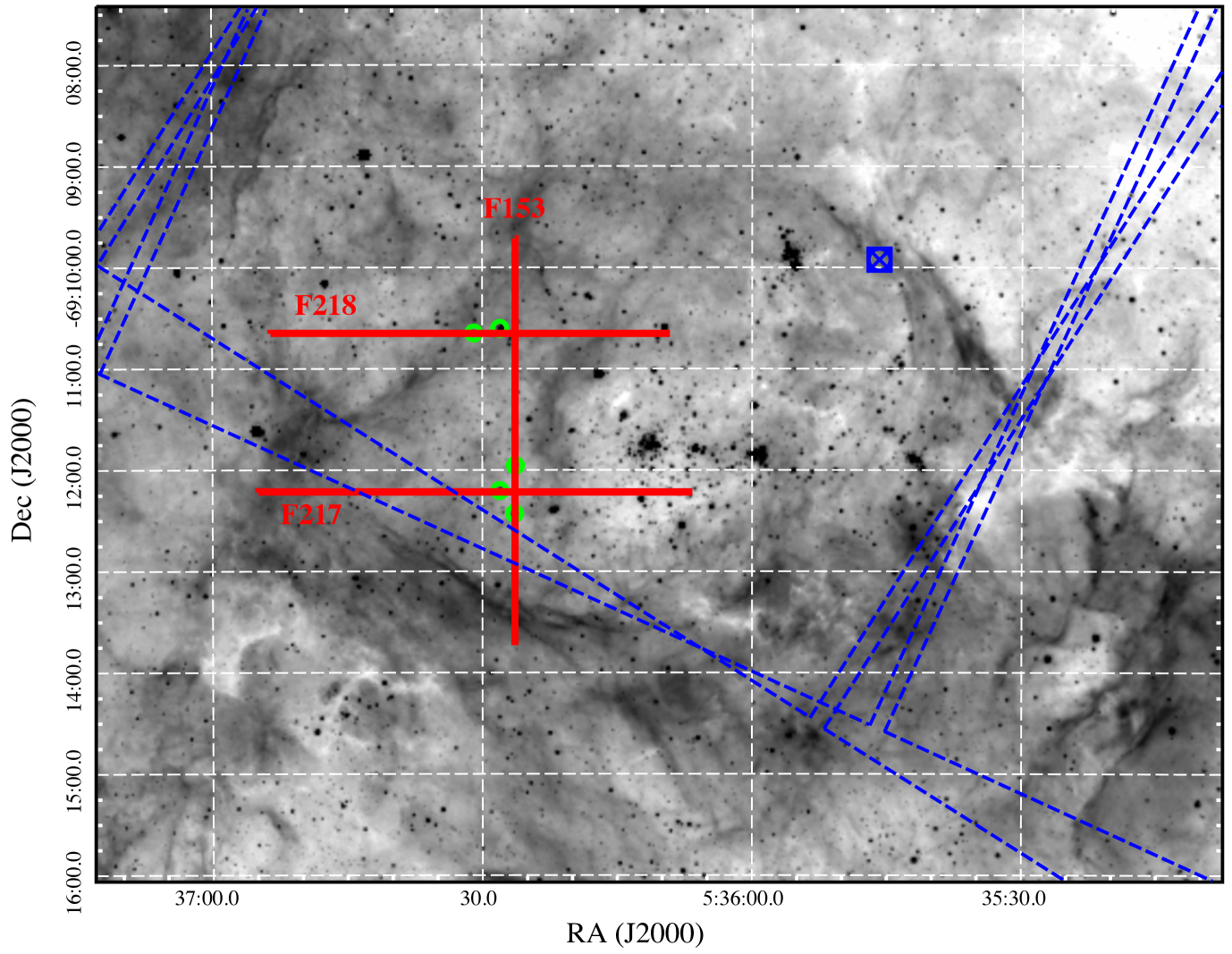
Figure 2: MCELS2 H$\alpha$ image of 30 Dor C. The positions of optical spectroscopic slits are indicated by the red lines. The contaminating point sources are marked by the green circles. The blue circle-cross point marks the aim-point of the Chandra observations with the blue dashed lines delineating the ACIS-S coverage.

2.2.2 Spectroscopy

Long-slit spectroscopy of the 30 Dor C shell has been performed in the past (Chu & Kennicutt 1988; Chu 1997). To aid in our analysis and discussion, we made use of the spectroscopic data of Chu (1997). These data were obtained using the spectrograph on the CTIO Blanco 4 m telescope. Two slits were aligned in the east-west direction with one aligned in the north-south direction, as showing in Fig. 2. The data were reduced using the standard IRAF tasks to produce the spectro-images shown in Fig. 3. The H$\alpha$ line is clearly visible in the spectro-images at $\approx 6569$ Å. Emission lines from [N_II] $\lambda 6548$ and [N_II] $\lambda 6583$ are also observed and are indicated in Fig. 3. In addition, continua from stars located in the slits are evident as the horizontal lines in the spectro-images. The contaminating stars are indicated in Fig. 2.

2.3 Radio continuum

We searched the Australia Telescope Online Archive database for high resolution, and high dynamic range observations of this region. 30 Dor C is about $5\arcmin$ away from SN1987A which is one of the most frequently observed ATCA sources. We used ATCA project C015 and we reduced the most recent (publicly available) ATCA CABB observations at 6 cm (5.5 GHz) which spans dates between 2010 and 2014. The observations totaled 77.68 hours time on source over 10 separate days. These observations are centered at SN1987A (Ng et al. 2013) with a number of different arrays including 6A, 6B, and 1.5A. The data reduction was done using the MIRIAD software package (Sault et al. 1995) and the final image used a Briggs robust weighting of 0.5 toward natural weighting. We combined all of these observations to and achieved an r.m.s. noise of $12\leavevmode\nobreak\ \mu$Jy/beam and resolution of $1.96\arcsec\times 1.71\arcsec$. While still suffering from the missing short spacings this image showed excellent dynamic range and filamentary structure along the western rim of 30 Dor C.

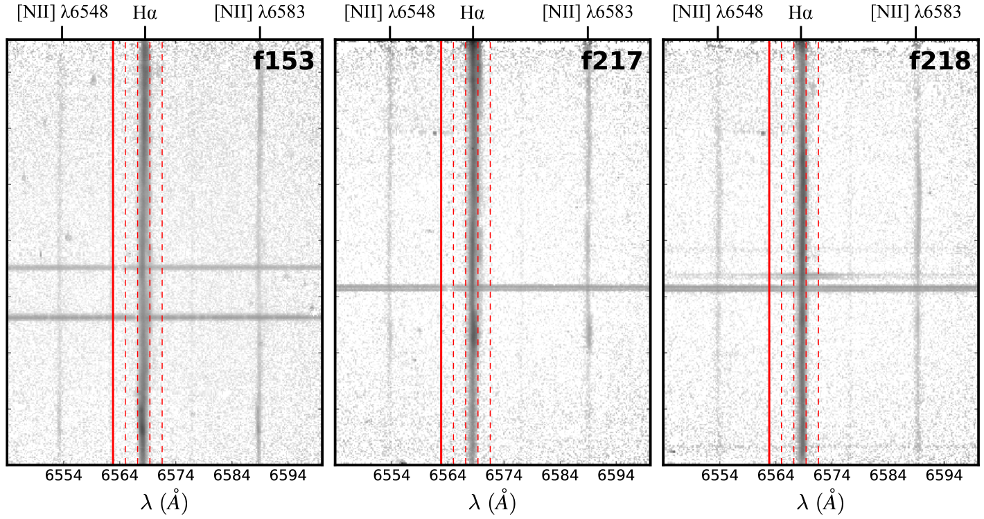
Figure 3: Spectro-images for each of the slit positions in Fig. 2 from Chu (1997). Emission lines from H$\alpha$ and [N_II] are indicated. The solid red line indicates the rest wavelength of H$\alpha$, while the dashed red lines indicate redshifted positions with recessional velocities from 100–400 km s^-1 in steps of 100 km s^-1. Note that the horizontal lines in each image are the continua of stars in the slits, marked by the green circles in Fig. 2.

2.4 Infrared

The cold environment surrounding 30 Dor C is revealed by infrared (IR) emission. To aid in the discussion of the morphology, we made use of data from the SAGE survey of the LMC (Meixner et al. 2006) with the Spitzer Space Telescope (Werner et al. 2004). During the SAGE survey, a 7°$\times$7° area of the LMC was observed with the Infrared Array Camera (IRAC, Fazio et al. 2004) in the 3.6 $\mu$m, 4.5 $\mu$m, 5.8 $\mu$m, and 8 $\mu$m bands, and with the Multiband Imaging Photometer (MIPS, Rieke et al. 2004) in the 24 $\mu$m, 70 $\mu$m, and 160 $\mu$m bands. The MIPS 24 $\mu$m images provide us with a picture of the stochastically and thermally heated dust in the region of 30 Dor C to give an indication of the distribution of cool material. We obtained the 24 $\mu$m MIPS mosaicked, flux-calibrated (in units of MJy sr^-1) images processed by the SAGE team from the NASA/IPAC Infrared Science Archive. The pixel sizes correspond to $4.8\arcsec$ for the 24 $\mu$m band, $\sim 1.2$ pc at the LMC distance.

3 Analysis

3.1 Expansion velocity of the H$\alpha$ shell

Both Chu & Kennicutt (1988) and Chu (1997) searched for high velocity material at various regions around the shell of 30 Dor C using long-slit optical spectroscopy. However, in both cases, only velocities $<100$ km s^-1 were observed, as illustrated in Fig. 3 using the same spectroscopic data of Chu (1997). The H$\alpha$ line in each of the spectro-images falls predominately in the 200–300 km s^-1 range, consistent with the systemic velocity of the LMC (250–300 km s^-1, Richter et al. 1987). Some structure can be seen in the H$\alpha$ line, but never with a velocity of more that 100 km s^-1 from the centroid of the line. As noted in Chu & Kennicutt (1988) and Chu (1997), this suggests that the H$\alpha$ shell of 30 Dor C is expanding at a rate consistent with an evolving superbubble rather than a supernova remnant. Note also that the presence of [N_II] $\lambda 6548$ and [N_II] $\lambda 6583$ in the spectra is indicative of radiative shocks, which occur only for low velocity shocks ($\lesssim 200$ km s^-1, Blair & Raymond 2017).

3.2 Measurement of the B-field

As we will discuss in Sect. 4.1, the synchrotron shell of 30 Dor C results from a SNR that has evolved inside the superbubble. The forward shock has expanded into the hot ($\sim 10^{6}$ K), rarefied medium which must have a density of $\sim 10^{-3}$ cm^-3. Indeed, assuming an explosion site at the centre of 30 Dor C, HC15 found that for a current shock velocity of $\gtrsim 3000$ km s^-1 to produce synchrotron X-rays, an interior density of $\sim 5\times 10^{-4}$ cm^-3 is required. As shown in Weaver et al. (1977) and in recent 3D hydrodynamical simulations by Krause et al. (2018), for young superbubbles expanding into a homogeneous environment, the interior density profile is more or less flat until very close to the supershell. Therefore, it is likely that the SNR has and continues to evolve into a relatively homogeneous medium of very low density and high temperature, accelerating VHE electrons which give rise to the filaments via synchrotron losses in the downstream region as is typical of field SNRs.

Helder et al. (2012) give an equation (their equation 26) relating the observed filament width to the postshock B-field:

$$B_{2}\approx 26\left(\frac{l_{\mathrm{adv}}}{1.0\times 10^{18}\leavevmode\nobreak\ \mathrm{cm}}\right)^{-2/3}\eta^{1/3}_{\mathrm{g}}\left(r_{4}-\frac{1}{4}\right)^{-1/3}\mu\mathrm{G},$$ (1)

where, the energy-dependent, $\eta_{\mathrm{g}}\equiv\lambda_{\mathrm{mfp}}/r_{\mathrm{g}}$, i.e., the ratio between the particle’s mean free path and the gyroradius, and $r_{4}$ is the shock-compression ratio in units of 4. This equation has been derived by balancing the acceleration time scale with the synchrotron loss time scale and, for that reason, also contains the shock compression factor (Helder et al. 2012). However, as shown in Helder et al. (2012) this condition is very similar to the condition that the advection length scale and diffusion length scale are equal, which leads to $l=\sqrt{D_{2}\tau_{\mathrm{syn}}}$, which gives a nearly identical expression (c.f. Völk et al. 2005; Vink et al. 2006; Rettig & Pohl 2012; Ressler et al. 2014). Similar to X-ray synchrotron spectra of various young supernova remnants, the X-ray synchrotron spectra of 30 Dor C ($\Gamma=2-3$, Bamba et al. 2004, see below also) are steeper than expected for diffusive shock acceleration and indicates that the spectra are indeed steepened due to radiative losses and must be near the spectral cut-off, justifying the use of Eq. 1. Moreover, $\eta_{\mathrm{g}}$ must be close to unity as for shock velocities below $5000\leavevmode\nobreak\ \mathrm{km\ s^{-1}}$ X-ray synchrotron radiation can only be produced for $\eta\lesssim 10$ (e.g. Zirakashvili & Aharonian 2007; Helder et al. 2012). In Appendix A we discuss how our magnetic field estimates might be affected if some of the underlying assumptions are not valid.

The actual width of the synchrotron emitting shell is somewhat larger than the advection/diffusion length scale $l_{\mathrm{obs}}\approx\sqrt{2}l_{\mathrm{adv}}$, with the factor $\sqrt{2}$ taking into account the combination of diffusion and advection. However, we cannot simply measure $l_{\mathrm{obs}}$ from the Chandra images since the surface brightness profile we observe is the projection of the volumetric emissivity profile onto the plane of the sky. As described in Willingale et al. (1996), assuming a spherically symmetric shell and that the shell plasma is optically thin, the surface brightness $\sigma(r_{p})$ at radius $r_{p}$ can be determined from the volumetric emissivity profile $\epsilon(r)$ using the forward Abel transform:

$$\sigma(r_{p})=2\int^{R}_{r_{p}}\frac{\epsilon(r)r}{(r^{2}-r^{2}_{p})^{1/2}}dr$$ (2)

where $R$ is the radius of the shell. We applied the forward Abel transform using the PyAbel Python package. For the volumetric emissivity $\epsilon(r)$, we assumed a simple model of an instantaneous rise at $R$, followed by an exponential fall-off in the postshock region:

$$\epsilon(r)=\begin{cases}A\leavevmode\nobreak\ \mathrm{exp}(-(r-R)/l_{\mathrm{obs}})+b_{u},&r<R\\ b_{u},&r>R\end{cases}$$ (3)

where $A$ is a normalisation factor (illustrated in Fig. 4, top-row), and $b_{u}$ is the upstream background level.

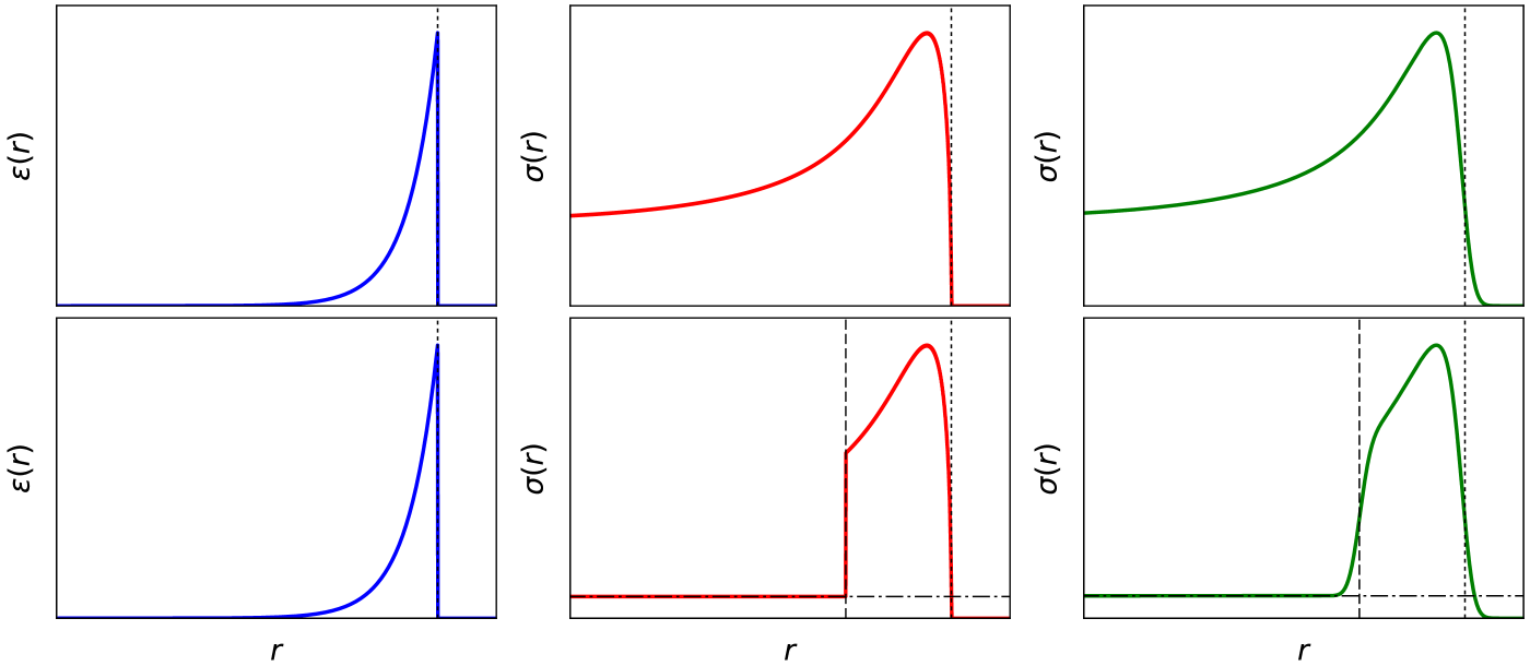
Figure 4: Illustration of projected and convolved volumetric emissivity profiles fitted to the segment profiles. Top-row: Postshock volumetric emissivity profile with radius $R$ (dotted lines) in Eq. 3 (left), projected emissivity profile using Eq. 2 (middle), and convolved with the PSF (right). Bottom-row: Same as top but for the projected ‘cap’ model in Eq. 4. The same postshock volumetric emissivity profile is used (left). The projected emissivity profile is modified to fall to a fitted background value $b$ (dash-dot lines) below $r_{f}$ which is a fraction $r_{c}$ of the shell radius $R$, $r<r_{f}=r_{c}R$ (middle, dashed lines). This was then convolved with the PSF (right).

The observed profile is also subject to smearing by the telescope’s PSF. Since the Chandra PSF varies as a function of position and energy, we must allow for this variation when convolving $\sigma(r_{p})$ with the PSF. We did this by calculating a monoenergetic PSF, set at 2.5 keV to be in the 1.5–8 keV range used for the profiles (see below), at the centre of each radial profile bin in each exposure using the MARX ray-tracing software (Davis et al. 2012). These PSFs were then weighted according to the exposure time of each exposure, added, and normalised. For each bin, we fitted the resulting PSF with a 2D Gaussian model and extracted a 1D profile across this model at the same position angle as the radial profile extracted from the Chandra data. Fitting this with a 1D Gaussian model provided an approximate PSF width at each position along the profile. These widths were used to perform a variable width convolution of the model profiles using the Varconvolve Python package.

To extract radial profiles from the data we defined sectors, centred on the 30 Dor C shell centre, taken from SY17, which are shown in Fig. 5. We masked the point sources, listed in Table 1, and interior enhancements that contaminated the ‘clean’ shell profiles such as filaments projected on the interior. We extracted profiles from the combined 1.5–8 keV exposure corrected, count rate image. We set our bin sizes so that each bin had a signal-to-noise ratio $>5$ (listed in Tables 2 and 3), but we omitted bins towards the centre of the shell because of low count rates and statistics. Sectors S8 and S9 were the only sectors in our sample which crossed the chip gap between the back-illuminated ACIS-S3 and front-illuminated ACIS-S4 chips. Because of the variation in sensitivity across the gap, we decided to cut the sectors and only consider the profile bins on the ACIS-S4 chip, where the brightest shell emission resides (see Fig. 5). We did not define sectors in the region between sectors S7 and S8 as the brightest emission in this region falls along the chip gap. We determined the integrated photon flux in each bin and normalised for the bin area to give radial profiles in surface brightness in units of counts cm^-2 s^-1 arcsec^-2.

To demonstrate that the $\Gamma$ values are indeed steep, must be near the spectral cut-off and that we could apply Eq. 1 to determine the B-field strength, we extracted and fitted spectra from each of the sectors to determine their $\Gamma$. However we were somewhat limited by the number of counts in the majority of sectors, resulting poorly constrained values of $\Gamma$. However, much deeper observations and analyses reported in the literature do provide a good indication the values of $\Gamma$ around the shell. We used the studies of KS15 and the more recent Babazaki et al. (2018) with XMM-Newton to determine indicative values of $\Gamma$ in our sectors. This resulted in $\Gamma\approx$ 2.7, 2.5, 2.6, 2.4, 2.4, 2.3, 2.4, 2.5, and 2.5 for sectors S1–S9, respectively, with a typical error of $\lesssim 0.1$ .

We fitted the projected and convolved volumetric emissivity profiles to the observed radial profiles allowing the values of $A$, $R$, and $l_{\mathrm{obs}}$ to vary. We determined the best-fit using $\chi^{2}$ minimisation and estimated 90% confidence intervals for those fits with reduced-$\chi^{2}$ less than 2 ($\chi^{2}_{\nu}<2$). This postshock model provided a good fit to most of our sectors, the results of which are given in Table 2 with the profiles and best-fit models shown in Fig. 6.

The postshock model did not provide a good fit to sectors S6 and S7, each giving a fit statistic of $\chi^{2}_{\nu}>2$. The S6 sector profile appeared to fall-off faster than would be expected from the postshock model. In an attempt to account for the shape of the observed profile, we modified the projected postshock profile to fall to $b_{u}$ at a fraction of the shell radius given by $r_{c}=r_{f}/R$, essentially modelling a spherical cap of emission. However, simply allowing the profile to fall to $b_{u}$ did not account for the flux observed in the inner most bins. This is somewhat expected as the interior 1.5–8 keV flux is much brighter and has more structure in the NW quadrant than anywhere else in 30 Dor C (e.g., KS15). Therefore, we included a second, interior background term $b_{i}$ (which represents $b_{u}$ plus the interior flux level) and allowed the profile to fall to $b_{i}$ in the innermost bins (e.g., Ressler et al. 2014). Therefore, we applied the model:

$$\sigma(r)=\begin{cases}b_{i},&r<r_{f}=r_{c}R\\ 2\int^{R}_{r_{p}}\frac{\epsilon(r)r}{(r^{2}-r^{2}_{p})^{1/2}}dr,&r>r_{f}=r_{c}R\\ \end{cases}$$ (4)

and allowed $r_{c}$ to vary in the fits. This model is illustrated in Fig. 4, bottom-row. This provided a better fit to sector S6, the results of which are given in Table 3 and the profile and best-fit model shown in Fig. 7. The cap model did not provide an acceptable fit for sector S7. We suspect that both the postshock and cap models fail to account for the profile because the shell in this sector is either not spherically symmetric, rendering the Abel transform invalid, there is too much interior structure to see a ‘clean’ shell profile, there is an additional source of synchrotron X-rays in addition to those from the postshock region, or because there is an apparent ‘pre-rise’ of the X-ray flux $\leavevmode\nobreak\ 10\arcsec$ ahead of the main filament, which could be a faster part of the shell seen in projection.

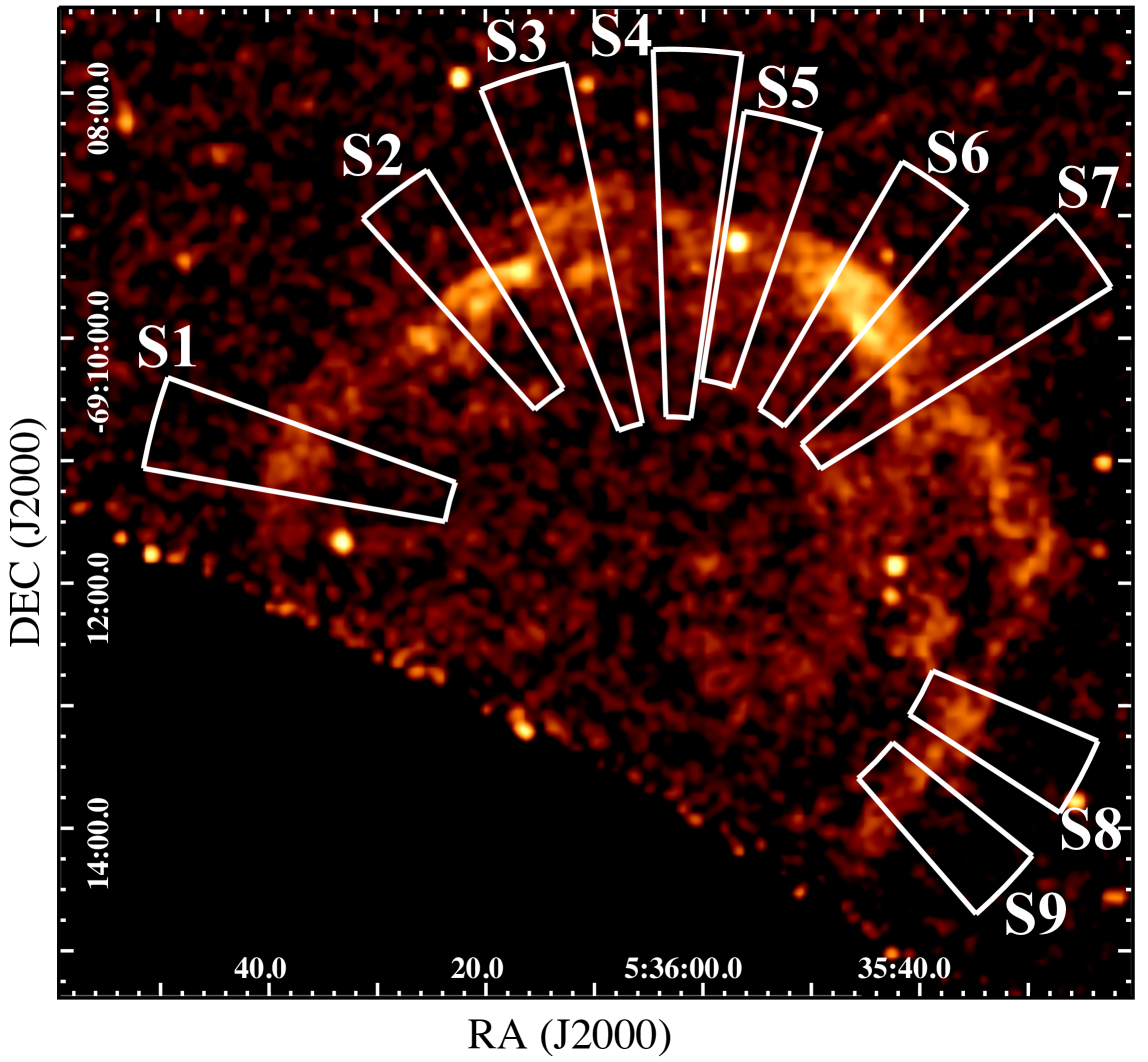
Figure 5: Segments for profile fitting overlaid on the 1.5–8 keV exposure corrected image. The image has been smoothed using a $3\sigma$ Gaussian kernel.

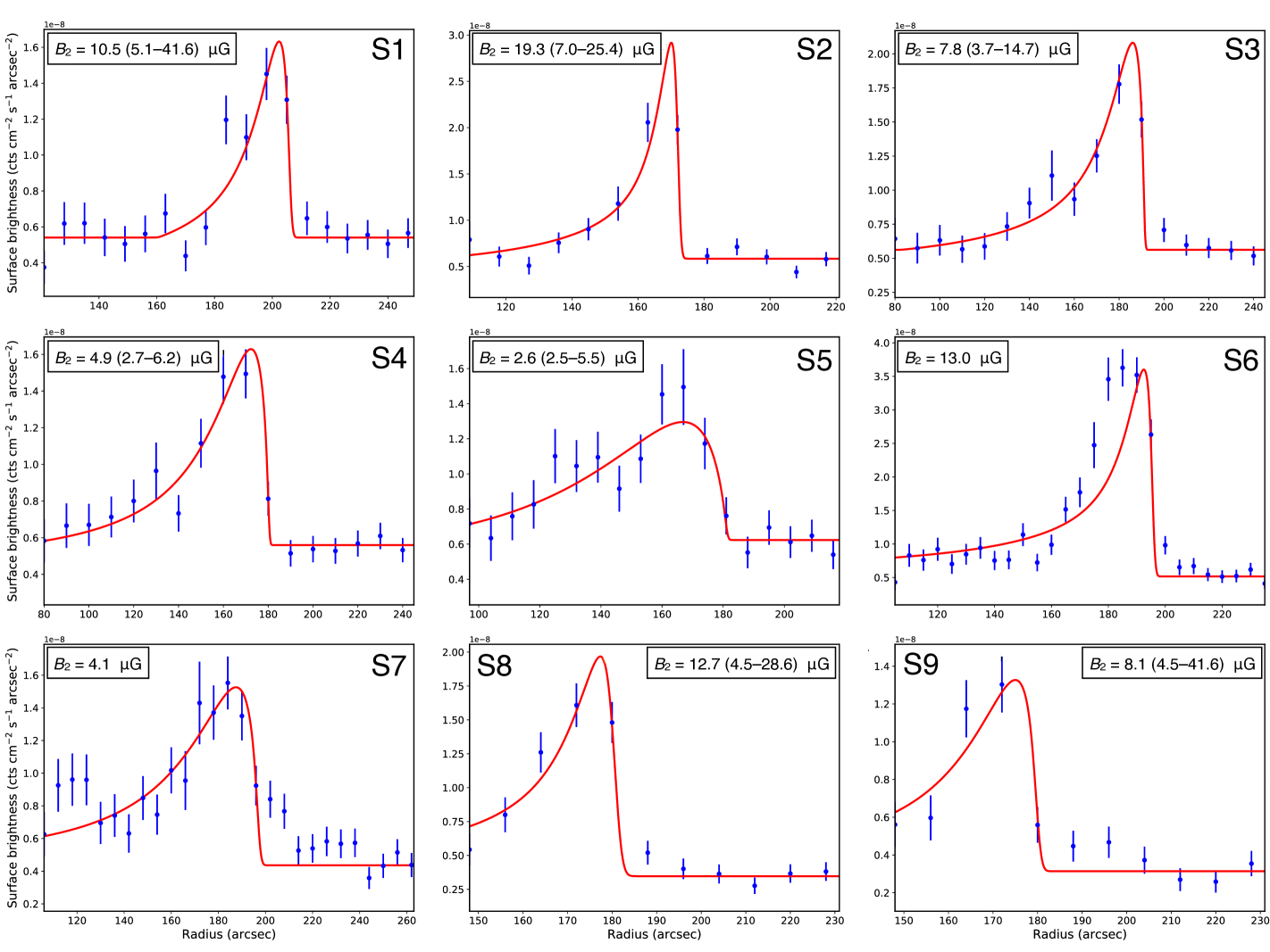
Figure 6: Radial profiles from sectors around 30 Dor C fitted with the postshock model described in Eq. 3. The best fit results are given in Table 2, with the determined $B$-fields indicated in the panels.

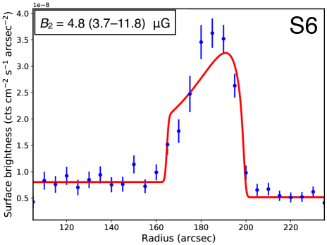
Figure 7: Radial profile from sector S6 fitted with the cap model. The best fit results are given in Table 3, with the determined $B$-field indicated.

Table 2: Postshock model (see Eq. 3) fits and B-field estimates in 30 Dor C. The numbers in parentheses correspond to the 90% confidence intervals of the fit parameters. Confidence intervals are only given for fits with $\chi^{2}_{\nu}<2$.

Sector	binning	$R$	$l_{\mathrm{obs}}$	$l_{\mathrm{obs}}/R$	$\chi^{2}_{\nu}$	$B_{2}$
	(arcsec)	(arcsec)	(arcsec)	(%)		($\mu G$)
S1	7	206.5 (204.5–212.7)	4.7 (1.2–9.6)	2.3 (0.6–4.7)	$1.20_{17}$	10.5 (5.1–41.6)
S2	9	172.6 (172.6–178.5)	2.6 (1.9–7.0)	1.5 (1.1–4.1)	$1.36_{11}$	19.3 (7.0–25.4)
S3	10	191.5 (190.6–198.0)	6.3 (3.3–13.3)	3.3 (1.7–7.0)	$0.59_{15}$	7.9 (3.7–14.7)
S4	10	180.8 (180.0–182.6)	10.1 (7.9–18.5)	5.6 (4.3–10.2)	$1.51_{15}$	4.9 (2.7–6.2)
S5	7	182.8 (175.9–183.7)	19.3 (9.0–20.1)	10.6 (4.9–11.4)	$0.69_{16}$	2.6 (2.5–5.5)
S6	5	195.8	3.8	1.9	$3.81_{25}$	13.0
S7	6	197.6	11.9	6.0	$2.07_{25}$	4.1
S8	8	181.2 (180.3–188.3)	3.9 (1.7–10.9)	2.2 (0.9–6.0)	$1.14_{9}$	12.7 (4.5–28.6)
S9	8	180.3 (172.3–181.2)	6.1 (1.2–10.9)	3.4 (0.7–6.3)	$1.51_{9}$	8.1 (4.5–41.6)

Table 3: Cap model (see Eq. 4) fits and B-field estimates in 30 Dor C. The numbers in parentheses correspond to the 90% confidence intervals of the fit parameters. Confidence intervals are only given for fits with $\chi^{2}_{\nu}<2$.

Sector	$R$	$l_{\mathrm{obs}}$	$r_{c}$	$l_{\mathrm{obs}}/R$	$\chi^{2}_{\nu}$	$B_{2}$
	(arcsec)	(arcsec)		(%)		($\mu G$)
S6	198.1 (195.7–199.6)	10.3 (4.2–13.2)	0.82 (0.81–0.84)	5.2 (2.1–6.7)	$1.86_{24}$	4.8 (3.7–11.8)

4 Discussion

4.1 Multi-wavelength morphology

The new Chandra, MCELS2 H$\alpha$, and 6 cm radio continuum images provide us with the sharpest view of the brightest regions of the shell of 30 Dor C to date. In Fig. 8 we show three-colour images comprising 24 $\mu$m, H$\alpha$  and 1.5–8 keV for RGB, for the northeast (NE, top-left), northwest (NW, top-right), southeast (SE, bottom-left), and southwest (SW, bottom-right). The 24 $\mu$m is included to highlight colder material in and around the shell. Interestingly, comparing the X-ray and H$\alpha$ emission in the NE, NW, and SE suggests that the X-ray and H$\alpha$ shells are not correlated, as was suggested by KS15 using poorer resolution XMM-Newton and MCELS data. Rather, the synchrotron X-rays fill gaps in the H$\alpha$ shell in some regions (NE, NW) and are located ahead of the H$\alpha$ shell in others (NW, SE). There are notable morphological consistencies in the NE and NW regions in particular with bright X-ray filaments delineating the edges of filaments in the H$\alpha$ shell, further highlighted in Fig. 9. There is also little correlation between the colder material revealed in 24 $\mu$m and the synchrotron X-ray shell. Rather, the X-rays appear brighter in regions with comparatively lower levels of infrared emission.

We show the high spatial resolution 6 cm radio continuum image along with the 24 $\mu$m and MCELS2 H$\alpha$ in an RGB image in Fig. 10. The radio continuum data bear a striking similarity to the H$\alpha$ emission, particularly along the filaments of the NW shell. Indeed, the only deviation along the brightest filament is in regions where foreground dust, revealed by the 24 $\mu$m emission, absorbs the H$\alpha$ emission. Therefore, the radio continuum must be thermal in origin and have little or no relation to the expanding X-ray synchrotron shell, also seen in other LMC superbubbles such as LHA 120-N 70 (De Horta et al. 2014).

As discussed in Sect. 3.1, the expansion velocity of the H$\alpha$ shell is $<100$ km s^-1, much less than the expansion velocity of the interior SNR required to explain the synchrotron X-rays ($\gtrsim 3000$ km s^-1, Zirakashvili & Aharonian 2007), as seen, for example, in the prototypical synchrotron-dominated SNR~RX~J1713.6-3946 (Acero et al. 2017b). The observed anti-correlation of the X-ray and H$\alpha$ shells does suggest a resolution to this expansion velocity conflict. It is possible that the SNR responsible for the synchrotron X-ray shell has reached the H$\alpha$ shell and has stalled in some regions, but continues through gaps in the H$\alpha$ shell in others, and explains why the H$\alpha$ shell is expanding at a rate typical of SBs whereas the SNR shell maintains the $\gtrsim 3000$ km s^-1 necessary to produce X-ray synchrotron emission. In addition, the bright 24 $\mu$m emission in the north, located between the bright regions of the X-ray synchrotron shell in the NE and NW (see Fig. 8, top-right), corresponds to a region of high radio polarisation (KS15, Fig. 7). This also supports the scenario that the expanding shock has met and compressed denser material in the north but continues to expand rapidly in the NE and NW.

The anti-correlation between H$\alpha$ and X-ray synchrotron emission is reminiscent of a similar anti-correlation in Tycho's SNR and RCW 86. For Tycho’s SNR the non-radiative H$\alpha$ filaments are more concentrated on the eastern side, whereas the synchrotron filaments are on the western side (Hwang et al. 2002). It has been speculated that this anti-correlation in caused by the damping of Alfvén waves if the neutral fraction is too high, which then leads to a suppression of turbulence necessary for the fast particle acceleration that gives rise to X-ray synchrotron emission. In RCW 86 a similar mechanism may also be at work, but it is more likely that the anti-correlation is caused by large velocity gradients along the shock wave (Vink et al. 2006; Helder et al. 2013). The contrast in velocity in RCW 86 is very large, which has been attributed to the fact that this remnant evolves in a wind-blown cavity (Vink et al. 2006; Williams et al. 2011; Broersen et al. 2014). In the SW of the remnant shock velocities are lower than 500 km s^-1, whereas in the NE, at the location of X-ray synchrotron emission, the shock velocity has recently been measured to be $\sim$3000 km s^-1 (Yamaguchi et al. 2016). In the same region there are patches of H$\alpha$ emission, but these appear to be slower than the X-ray synchrotron filaments, with a mean velocity $\sim 1200$ km s^-1 (Helder et al. 2013).

The anti-correlation in 30 Dor C, with its measured velocity contrasts, seems therefore to be a result of the same processes as in RCW 86, but even more extremely so. If the X-ray synchrotron filaments are the result of a single supernova explosion going off in the extremely tenuous interior of a superbubble, the extreme velocity contrast may be caused by density gradients and the fact that the shock radius is so much larger, $\sim 50$ pc (e.g., Sano et al. 2017), that most of the shock energy has been distributed over a large shock area, making it more sensitive to density gradients.

The difference in X-ray morphology between 30 Dor C and other superbubbles has been discussed by various authors (e.g., BU04, KS15). The rim-brightened morphology and hard X-rays of 30 Dor C contrasts the more ‘typical’ picture of a superbubble with a centrally-filled soft X-ray morphology, such as N~70 (Zhang et al. 2014). However, the optical and radio properties of 30 Dor C are consistent with other LMC superbubbles. The anti-correlation between synchrotron X-ray and H$\alpha$ shell presented in this work supports that 30 Dor C is similar to other superbubbles but only special in that we are seeing a recent SN in the interior (see also discussions in BU04, HC15, for examples).

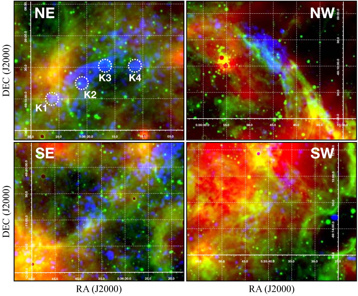
Figure 8: False-colour image of the 30 Dor C shell in the NE (top-left), NW (top-right), SE (bottom-left), and SW (bottom-right) with RGB = 24 $\mu$m, H$\alpha$, 1.5–8 keV. Knots K1–K4 are shown in the NE shell.

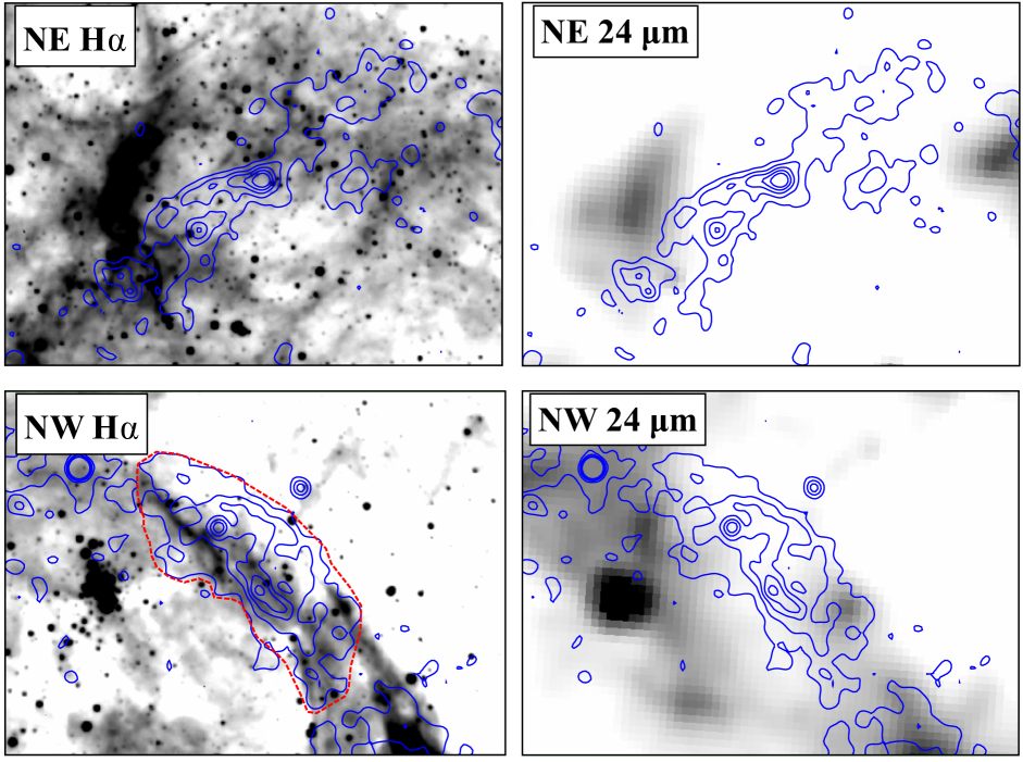
Figure 9: MCELS2 H$\alpha$ and 24 $\mu$m images of the NE and NW shells of 30 Dor C with 1.5–8 keV contours overlaid. The contour levels were manually set to highlight the brightest regions of the synchrotron shell. The red region overlaid on the NW H$\alpha$ image in bottom-left corresponds to the spectral extraction region used in Sect. 4.3.

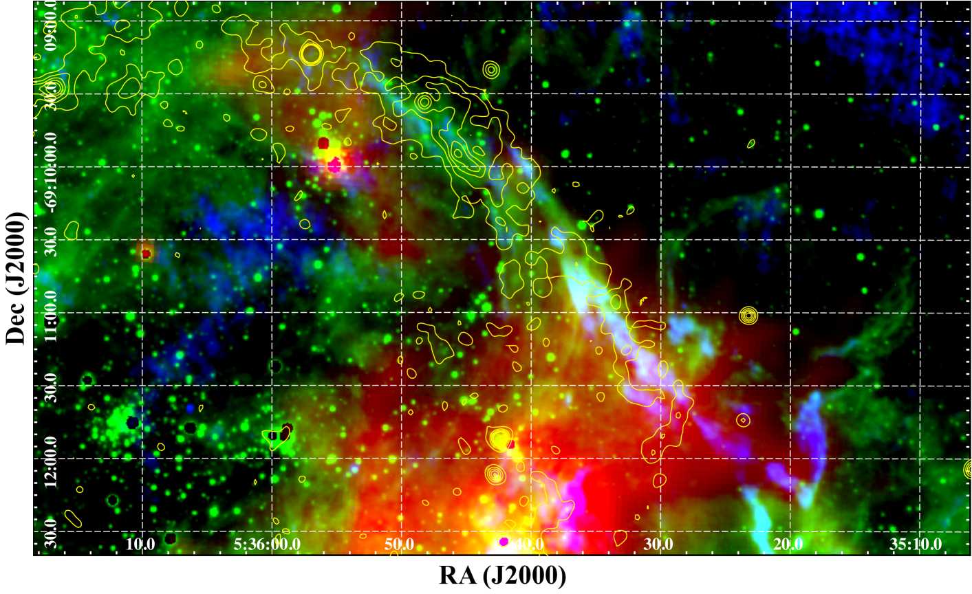
Figure 10: False-colour image of the 30 Dor C shell in the NW with RGB = 24 $\mu$m, H$\alpha$, 6 cm radio continuum. The contours shown in yellow are the 1.5–8 keV contours from Fig. 9. The extended 6 cm emission seen interior to the NW shell and in the top-right of the image is due to the edge of the primary beam.

4.2 B-field for hadronic models

To estimate a lower limit for the B-field for a hadronic dominant TeV emission, we ran a set of hybrid models and compared these to the spectral energy distribution of 30 Dor C shown in HC15 (their Fig. 3) to illustrate how an increasing hadronic contribution to the TeV emission also requires an increasing B-field. We show these models in Fig. 11, along with the purely leptonic model from HC15. As the energy in protons, relative to electrons, is increased, the B-field required to fit the synchrotron X-rays also increases. For the hybrid model with completely dominant hadronic TeV emission ($>$90%), a B-field of $\gtrsim 50\leavevmode\nobreak\ \mu$G is needed to account for the X-ray emission. The model with a 50-50 contribution to the TeV emission requires a B-field of $\sim 20\leavevmode\nobreak\ \mu$G.

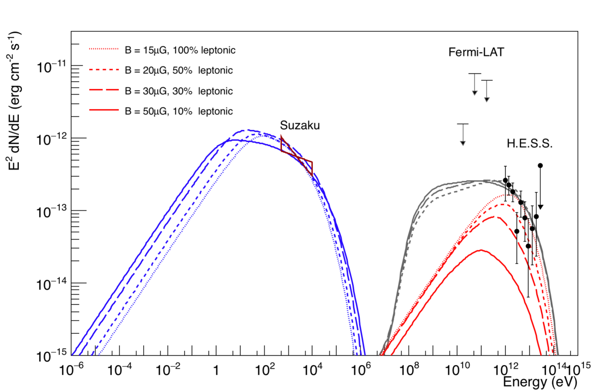
Figure 11: Three hybrid models and the pure leptonic model from HC15 applied to the SED of 30 Dor C described in HC15. The blue lines show the synchrotron component, the red lines show the contribution of IC in the TeV domain, while the grey lines show the IC+hadronic component. The solid lines are for energy in protons $E_{p}=1.50\times 10^{50}$ erg, energy in electrons $E_{e}=2.25\times 10^{48}$ erg, $B=50\leavevmode\nobreak\ \mu\mathrm{G}$, long-dashed lines for $E_{p}=1.25\times 10^{50}$ erg, $E_{e}=3.40\times 10^{48}$ erg, $B=30\leavevmode\nobreak\ \mu\mathrm{G}$, short-dashed lines for $E_{p}=1.00\times 10^{50}$ erg, $E_{e}=3.50\times 10^{48}$ erg, $B=20\leavevmode\nobreak\ \mu\mathrm{G}$, and the dotted line is the pure leptonic model from HC15 with $B\sim 15\leavevmode\nobreak\ \mu\mathrm{G}$. An increasing B-field is required to account for the X-ray emission when the energy in protons, relative to electrons, is increased.

4.3 Synchrotron profiles

In Sect. 3.2, we described the extraction of synchrotron emission profiles from various sectors around the shell and their modelling with a radial profile as typically seen from SNRs, i.e., an instantaneous rise at shell radius $R$, followed by an exponential fall-off in the postshock region and assuming the shell is spherically symmetric. In almost all sectors (S1, S2, S3, S4, S5, S8, and S9), this model provided a good fit to the radial profiles. The fact that the profiles fit this SNR model in most regions of 30 Dor C, and the anti-correlation between H$\alpha$/ 24 $\mu$m emission (Fig. 8) and X-ray synchrotron emission argue against the interpretation of SY17 that the synchrotron X-rays originate in the shock-cloud interaction regions. If this were the case, the observed profiles should be the sum of a multitude of very narrow synchrotron filaments in the various shock-cloud interaction regions, and there is no reason to expect that this would give rise to the SNR-type volumetric emissivity profile that provides a good fit to the data.

However, there are two sectors whose radial profiles are not well-fitted by the SNR model, i.e., sectors S6 and S7. Interestingly, these sectors cross the brightest region of the synchrotron shell which is correlated with the MC4 molecular cloud identified by SY17. Therefore, it is possible that some or all of the synchrotron emission in the brightest region could be due to VHE electrons in shock-cloud interaction regions. In Sect. 3.2 we showed that the S6 profile can be fitted using a modified ‘cap’ model. While this does provide an acceptable fit to the data, we have no reason to expect such an emission profile in this sector. In addition, some bright X-ray knots of emission were found in the NE shell, which were masked during the radial profile extraction. The origin of these knots, which are marked in Fig. 8 as knots K1 through K4, is unclear. If these knots resulted from enhanced emission at shock-cloud interaction regions, we might expect them, and the NW shell, to be variable on short timescales (Inoue et al. 2009) such as in supernova remnants such as Cas~A on timescales of a few years (Uchiyama & Aharonian 2008).

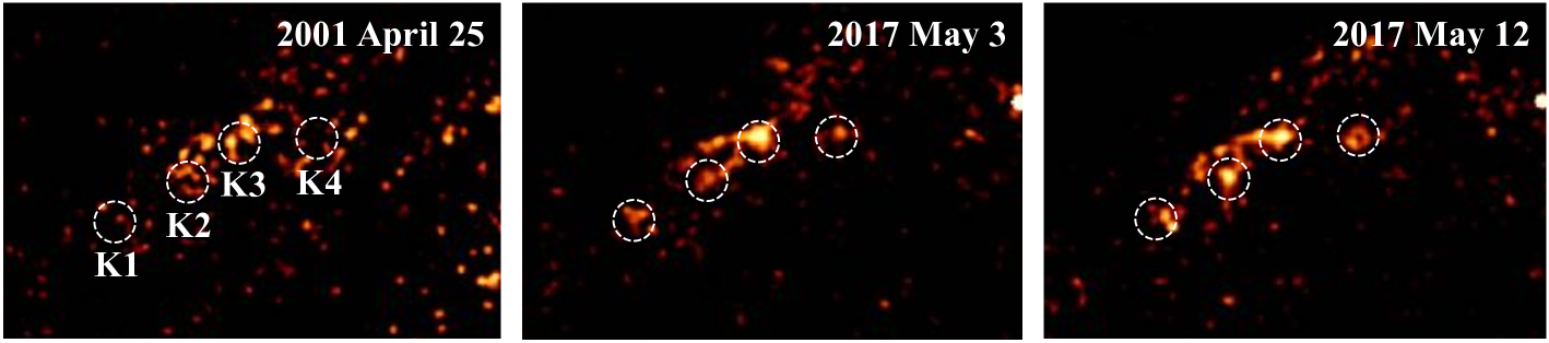
Figure 12: Chandra 1.5–8 keV flux corrected images of the NE shell over three epochs, which are indicated in the panels. Knots K1–K4 are shown on the plots. Each image has been smoothed using a 3$\sigma$ kernel to better show the diffuse structure. The colour scales in each panel are the same.

To search for variability, we used both epochs of our new Chandra observations (2017 May 3 and 2017 May 12) and the only other observation to cover the northern shell, taken in 2001 April (ObsID 1044, $\sim$18 ks, PI: G. Garmire) which were reported in BU04. We processed this dataset as described in Sect. 2.1. The target of ObsID 1044 was SN1987A, and, therefore, the NW and NE shells are located $\gtrsim$7’ off-axis, resulting in lower sensitivity and a degradation of the PSF. Flux-corrected and smoothed 1.5–8 keV images of the NW and NE shells in each epoch are shown in Fig. 12, along with the positions of the knots. We used the observed counts to determine the photon flux and error in each knot region for each epoch. We found for Obs. ID 1044 that the comparatively short exposure time of $\sim$18 ks, coupled with the off-axis location of the northern shell resulted in a small number of counts (¡20) per knot in the 1.5–8 keV range, prohibiting a robust variability study of the knots. In addition, the brightest region of the NW shell was located on an ACIS-S chip gap during ObsID 1044 so we could not reliably compare counts between the 2001 and 2017 epochs.

Interestingly, in the course of our variability study, we found that the NW shell region appeared to vary between the two 2017 epochs, i.e., on a timescale of nine days. The increase from $51.49\leavevmode\nobreak\ (\pm 2.40)\times 10^{-6}$ phot cm^-2 s^-1 on 2017 May 3 to $64.24\leavevmode\nobreak\ (\pm 2.52)\times 10^{-6}$ phot cm^-2 s^-1 on 2017 May 12 corresponds to a $\gtrsim 10$ % increase in flux, which is rather puzzling as synchrotron variability is not expected on such short timescales. Fluxes extracted from the other bright synchrotron region in the NE shell, located $\sim 2\arcmin$ away and also on the ACIS-S3 chip, showed no evidence of variability.

We further assessed the increase in flux and whether it was accompanied by a change in spectral shape, using spectral analysis. We extracted source (indicated in Fig. 9, bottom-left) and background spectra for the NW shell using the CIAO task specextract and fitted them using XSPEC (Arnaud 1996) version 12.8.2p with abundance tables set to those of Wilms et al. (2000), photoelectric absorption cross-sections set to those of Balucinska-Church & McCammon (1992). Detected point sources were masked. Since the spectrum of the NW shell has been found in all previous studies to be dominated by a single non-thermal component, we fitted the spectra with a power-law, absorbed by Galactic and LMC material (phabs*vphabs*pow in XSPEC), with the Galactic absorption fixed to $6\ \times\leavevmode\nobreak\ 10^{20}$ cm^-2 (Dickey & Lockman 1990) and the LMC absorption fixed to $1.0\ \times\ 10^{22}$ cm^-2 (KS15). We estimated fluxes and errors using the cflux convolution model component. Our spectral model provided a good fit in each epoch, and the data and best-fits are shown in Fig 13. The increase in flux between 2017 May 3 and 2017 May 12 is evident in the plot and the best-fit cflux parameters with $F_{\rm{X,1.5-8\leavevmode\nobreak\ keV}}=2.19\leavevmode\nobreak\ (1.95-2.39)\times 10^{-12}$ erg cm² s^-1 for 2017 May 3 and $F_{\rm{X,1.5-8\leavevmode\nobreak\ keV}}=2.95\leavevmode\nobreak\ (2.69-3.16)\times 10^{-12}$ erg cm² s^-1 for 2017 May 12. The best-fit photon index ($\Gamma$) of the power-law component does decrease between the epochs, however we cannot conclude that this is in fact the case as the indices are consistent within the 90% confidence intervals for 2017 May 3 and 2017 May 12 at $\Gamma_{2017-05-03}=2.55\leavevmode\nobreak\ (2.41-2.70)$ and $\Gamma_{2017-05-12}=2.32\leavevmode\nobreak\ (2.20-2.44)$, respectively.

While the determined fluxes from the NW shell at the 2017 May 3 and 2017 May 12 epochs suggest an increase in brightness of the shell of $\gtrsim$10%, the currently available datasets cannot show that this is accompanied by a change in the spectrum. The abrupt increase in flux is very difficult to physically explain. Taking the observed widths of the S6 and S7 sectors of the synchrotron shell from Tables 2 and 3, the minimum width of the shell is $\sim 4\arcsec$ which corresponds to $\sim$1 pc at the LMC distance. Given this width, signal speeds faster than the speed of light would be required to explain a flux variability on timescales of days. We also assessed a possible systematic origin for the apparent flux increase. The bounds of the NW shell region are within an arcminute of the ACIS-S aimpoint. Other regions considered for variability in the NE are $2\arcmin-3\arcmin$ away but also on the S3 chip and no evidence of variability was found in these, ruling out some variation in detector background between the epochs. We also checked for variation in the NW background region, located outside the NW shell but no variation was found. As already noted, detected point sources were masked so the increase in flux is not due to a variable point source. Future deep Chandra observations would be required to verify if the apparent variability is real.

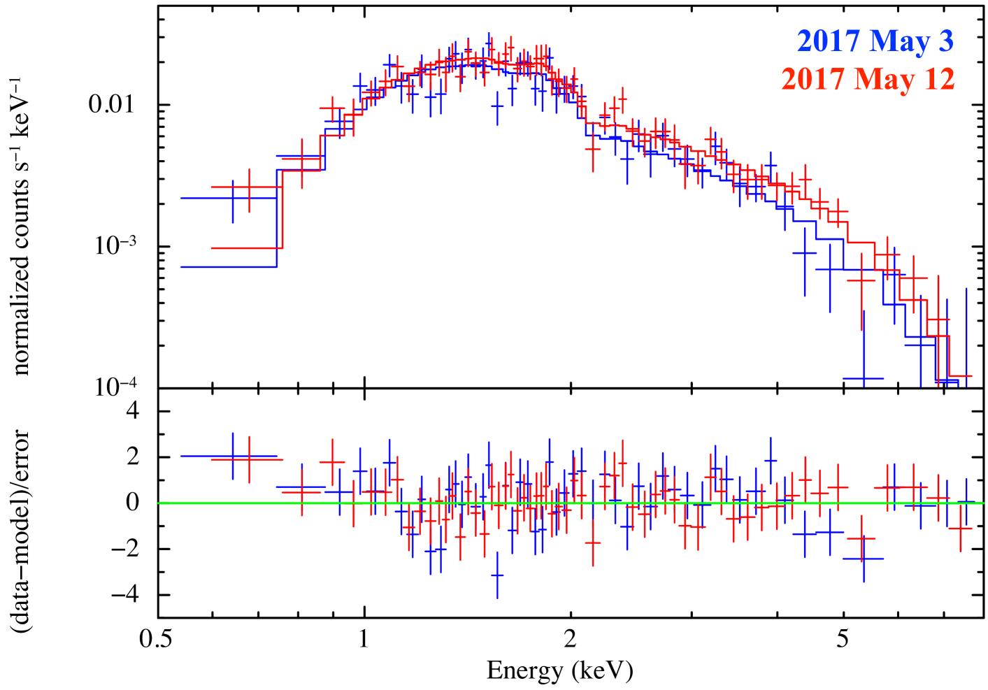
Figure 13: Spectra from the NW shell fitted with an absorbed power-law model. The spectrum from 2017 May 3 is shown in blue and that from 2017 May 12 in red.

4.4 B-field estimates and TeV emission mechanism

The estimated B-field in those sectors well-fitted by the SNR volumetric emissivity profile model is low with the best fit B-field strengths ranging from 2.6–19.3 $\mu$G (see Table 2). In three sectors the upper limits of the 90% confidence intervals extend beyond $\sim 30$ $\mu$G, though the estimates in these sectors are poorly constrained. Therefore, the shape of the profiles (discussed in the previous sub-section) and the determined B-field strengths suggest an SNR origin, where the average downstream magnetic field strength is consistent with a compressed ISM. These low magnetic field strengths suggest a leptonic-dominated origin for the TeV $\gamma$-rays detected by HC15 from 30 Dor C.

The upcoming Cherenkov Telescope Array (C.T.A., Cherenkov Telescope Array Consortium et al. 2017) will provide further constraints and verification of the TeV emission mechanism in 30 Dor C. Hadronic and leptonic mechanisms predict different flux for the (10 GeV–1 TeV) band, both currently below Fermi-LAT (Atwood et al. 2009; Ackermann et al. 2011) sensitivity and between Fermi and H.E.S.S. covered energy ranges, but within the capabilities of C.T.A. An example of the prospects of C.T.A. in this regard is shown by Acero et al. (2017a) as applied to the SNR RX J1713.7–3946. The recent H.E.S.S. paper on RX J1713-3946 (H. E. S. S. Collaboration et al. 2018) demonstrates the possibilities for C.T.A. observations of LMC objects. H.E.S.S. revealed the TeV shell of RX J1713.7–3946 in unprecedented detail, and was found to extend further than the X-ray shell. This allowed the probing of particle escape, while the GeV and TeV spectra were covered to a level of accuracy that allowed a very detailed comparison of leptonic and hadronic emission mechanisms, including a magnetic field map for the leptonic case.

5 Conclusion

We have presented an analysis of new Chandra observations of 30 Dor C in the Large Magellanic Cloud, the first superbubble detected in TeV $\gamma$-rays. These observations provided the sharpest view of the synchrotron X-ray shell of 30 Dor C, allowing us to perform a detailed morphological study and estimate the B-field in the superbubble, a key discriminator in assessing the dominant TeV $\gamma$-ray emission mechanism with a low $B$-field $\sim 15$ $\mu$G required for a purely leptonic origin, a $B$-field of $\gtrsim 50$ $\mu$G for a completely hadronic-dominated origin, or $B$-field of $\sim 20$ $\mu$G for a 50-50 contribution of the leptonic and hadronic mechanisms to the TeV $\gamma$-rays.

Using the new Chandra data, MCELS2 H$\alpha$, and 6 cm radio continuum images we found an anti-correlation between the synchrotron X-ray and H$\alpha$/6 cm shells. In addition, we discussed how long-slit spectroscopy of various regions of the 30 Dor C shell has shown no evidence of the high-velocities necessary to explain the synchrotron X-rays ($\gtrsim 3000$ km s^-1). Rather the H$\alpha$ expansion velocities are more typical of an expanding superbubble ($<100$ km s^-1). We suggested that the SNR responsible for the synchrotron X-rays has reached the 30 Dor C supershell and has stalled in some regions, but continues through gaps in the shell in others. This is similar to the observed anti-correlation seen in RCW 86 (Vink et al. 2006; Helder et al. 2013), which is attributed to the SNR evolving into a wind-blown cavity and encountering density gradients, though the velocity differences between synchrotron X-ray and H$\alpha$ shells are not as extreme. This may be a result of more pronounced density gradients and/or the fact that the shock radius is so much larger in 30 Dor C, meaning the shock energy has been distributed over a large area, making it more sensitive to these density gradients.

We estimated the downstream B-field from the synchrotron X-ray shell. This was achieved by fitting the observed radial profile in sectors around 30 Dor C with a typical postshock volumetric emissivity profile projected onto the sky and convolved with the Chandra PSF to determine the width of the shell. From this width we determined the B-field using Eq. 26 from Helder et al. (2012). We obtained good fits to the majority of the sectors with the postshock model and found that the downstream B-field was generally low, all with best fits $\lesssim 20\leavevmode\nobreak\ \mu$G, though upper confidence limits reaching $\gtrsim 30\leavevmode\nobreak\ \mu$G in three sectors where the confidence intervals were poorly constrained. This suggests that the TeV emission is likely dominated by IC emission, i.e., the leptonic scenario. Our postshock model did not provide good fits to two sectors. We found that one sector did not provide a ‘clean’ radial profile because of interior structure, while the other could be fitted with a modified projected postshock model where the projected profile falls off abruptly below $\sim 0.8$ times the shell radius, yielding a postshock B-field of 4.8 (3.7–11.8) $\mu$G which is again consistent with the leptonic TeV $\gamma$-ray mechanism. Alternatively, the observed profiles in these sectors could result from synchrotron enhancements around a shock-cloud interaction as suggested by SY17.

Appendix A Could the electron spectrum be age-limited instead of loss-limited?

In the main body of the text we showed that the widths of the X-ray synchrotron filaments are typically 5″ (5.8 pc or $1.8\times 10^{19}$ cm), which implies a magnetic field strength of $B\lesssim 15\mathrm{\mu G}$, based on Eq. 1. This low magnetic field implies that TeV $\gamma$-ray emission is dominated by inverse Compton scattering of background photons, rather than by pion production (H.E.S.S. Collaboration et al. 2015, see also Sect. 1). However, the magnetic field strength estimate relies on Eq. 1, and there may be some concern that the electron maximum energy is not limited by radiative losses.

A more general equation that relates the X-ray synchrotron width to magnetic field strength is the advection length scale, already alluded to in the main text:

$$l_{\mathrm{adv}}= <\Delta v>\tau_{\mathrm{syn}}=<\Delta v>\frac{9(m_{\mathrm{e}}c^{2})^{2}}{4e^{4}c}\frac{1}{B^{2}E_{\mathrm{e}}}\approx\frac{634}{B^{2}E_{\mathrm{e}}},$$ (5)

with $\sigma_{\mathrm{T}}$ the Thomson cross section, $m_{\mathrm{e}}$ the electron rest mass, $E_{\mathrm{e}}$ the electron energy, and $<\Delta v>$ the average advection velocity downstream of the shock. Normally we would assume that $<\Delta v>=V_{\mathrm{s}}/r$, with $r=4$ the shock compression ratio. However, here we will allow for gradients in velocity. This equation is generally applicable, but has the disadvantage that it depends on $<\Delta v>$, which we do not know, and on the typical electron energy, $E_{\mathrm{e}}$, at which we observe the shock. The latter can be estimated by using the relation between photon energy, electron energy, and magnetic field strength for synchrotron radiation (Ginzburg 1965): $E_{\mathrm{ph}}=7.4E_{\mathrm{e}}^{2}B$ keV (with $E_{\mathrm{e}}$ and $B$ in cgs units). This gives (see also Rettig & Pohl 2012):

$$l_{\mathrm{adv}}\approx 5.5\times 10^{18}\left(\frac{<\Delta v>}{1000\leavevmode\nobreak\ \mathrm{km\ s^{-1}}}\right)\left(\frac{E_{\mathrm{ph}}}{1\leavevmode\nobreak\ \mathrm{keV}}\right)^{-1/2}\left(\frac{B}{10\leavevmode\nobreak\ \mathrm{\mu G}}\right)^{-3/2}\leavevmode\nobreak\ \mathrm{cm};$$ (6)

or inverted:

$$B\approx 31\left(\frac{l}{1\times 10^{18}\leavevmode\nobreak\ \mathrm{cm}}\right)^{-2/3}\left(\frac{<\Delta v>}{1000\leavevmode\nobreak\ \mathrm{km\ s^{-1}}}\right)^{2/3}\left(\frac{E_{\mathrm{ph}}}{1\leavevmode\nobreak\ \mathrm{keV}}\right)^{-1/3}.$$ (7)

This expression has some similarities to Eq. 1, since that equation was also based on the advection length scale. It also shows that for photons around 1 keV and advection speeds of $\approx 1000\leavevmode\nobreak\ \mathrm{km\ s^{-1}}$, we get a very similar magnetic field strength. However, unlike for some young SNRs, such as Cas A (Vink & Laming 2003), we lack a measurement of the shock speed and thus an estimate of $<\Delta v>$. So the question then is whether $<\Delta v>\approx 1000\leavevmode\nobreak\ \mathrm{km\ s^{-1}}$ is indeed a good estimate for the advection velocity in the X-ray synchrotron filaments of 30 Dor C.

Superbubbles are expected to have expansion velocities of $30-200\leavevmode\nobreak\ \mathrm{km\ s^{-1}}$. This is consistent with the velocity information from the optical emission from 30 Dor C, which applies to the thermal X-ray emitting shell, not the X-ray synchrotron emitting shell. If we would assume these velocities, say $<\Delta v>\approx 100\leavevmode\nobreak\ \mathrm{km\ s^{-1}}$, the magnetic field estimate would come down to $B\sim 3\leavevmode\nobreak\ \mathrm{\mu G}$ or less. This would weaken the case for hadronic gamma-ray emission even more, but such a low velocity would be inconsistent with the emission of X-ray synchrotron radiation. A problem with much lower shock velocities is that they cannot produce X-ray synchrotron emission, as this generally requires $V_{\mathrm{s}}\gtrsim 3000\leavevmode\nobreak\ \mathrm{km\ s^{-1}}$ (e.g. Aharonian & Atoyan 1999; Zirakashvili & Aharonian 2007), corresponding to $\Delta v\gtrsim 750\leavevmode\nobreak\ \mathrm{km\ s^{-1}}$. This requirement relies on the assumption that acceleration gains balances radiative losses, but we note that letting go of this requirement generally leads to low magnetic fields. We illustrate this by using the approximate relation between shock speed, and the radius and age of a supernova remnants: $V_{\mathrm{s}}=mR/t$, with $t$ the age of the object and $0.4\leq m\leq 1$, with $m=0.4$ corresponding to the Sedov-Taylor solution and $m=1$ to free expansion (see for example the review Vink 2012). Now the requirement that the synchrotron loss time is longer than the age of the object implies:

$$t=\frac{mR}{V_{\mathrm{s}}}< \tau_{\mathrm{syn}}\approx\frac{634}{B^{2}E_{\mathrm{e}}}$$ (8)

$$\Rightarrow$$

$$B< 3.1m^{-2/3}\left(\frac{E_{\mathrm{ph}}}{1\leavevmode\nobreak\ \mathrm{keV}}\right)^{-1/3}\left(\frac{V_{\mathrm{s}}}{5000\leavevmode\nobreak\ \mathrm{km\ s^{-1}}}\right)^{2/3}\left(\frac{R}{50\leavevmode\nobreak\ \mathrm{pc}}\right)^{-2/3}\leavevmode\nobreak\ \mathrm{\mu G}.$$

So for an object the size of 30 Dor C the electron spectrum has to be loss limited, or the magnetic field has to be even lower than our best estimate. But if the spectrum is loss limited the current shock velocity has to be $V_{\mathrm{s}}\gtrsim 3000\leavevmode\nobreak\ \mathrm{km\ s^{-1}}$, or it has to have been that high in the recent past, i.e, less than a synchrotron loss time scale ago.

Looking at Eq. 7 we in fact see that the only way that our main conclusion, namely that the magnetic field strength is lower than $50\leavevmode\nobreak\ \mathrm{\mu G}$, can be wrong is if $<\Delta v>\gtrsim 3000\leavevmode\nobreak\ \mathrm{km\ s}^{-1}$, corresponding to $V_{\mathrm{s}}>12000\leavevmode\nobreak\ \mathrm{kms}^{-1}$. Although a very young SNR could have $V_{\mathrm{s}}\sim 12000\leavevmode\nobreak\ \mathrm{km\ s^{-1}}$, it would not maintain that velocity for long enough to inflate to a radius of 50 pc ($\sim 6$ kyr for $V_{\mathrm{s}}\sim 12000\leavevmode\nobreak\ \mathrm{km\ s^{-1}}$).

Given that $<\Delta v>\approx 1000\leavevmode\nobreak\ \mathrm{km\ s}^{-1}$ is in close agreement with expectations, and that Eq. 7 provides a very similar magnetic field estimate as Eq. 1, strengthens the reliability of our magnetic field estimates, and also provides evidence that $\eta_{\mathrm{g}}\lesssim 10$.

It should be noted that the magnetic field may be strongly position dependent, if magnetic field damping plays an important role, but also due to the divergent flow of the plasma. In the context of X-ray synchrotron emission from supernova remnants the potential role of magnetic field damping was first pointed out in Pohl et al. (2005). The idea is that the cosmic-ray induced magnetic field amplification (Bell 2004), which occurs in the cosmic-ray precursor, will decay again in the downstream region. In that case the narrow widths of the X-ray filaments may not so much reflect the advection length scale (Eqs. 1 and  6), but the typical decay length scale of the magnetic field. This idea was applied to young SNRs by Rettig & Pohl (2012) and to Tycho’s SNR by Tran et al. (2015). We have ignored the effect in our magnetic field estimate, but we note here that our main conclusion is that the magnetic field strength in 30 Dor C is lower than expected. Magnetic field damping leads to observed X-ray synchrotron filament widths that are smaller than advection/synchrotron loss models. In general, therefore, magnetic field estimates including damping lead to lower estimates of the magnetic strengths as reported by Rettig & Pohl (2012); Tran et al. (2015).

The effects of the divergent flow on the magnetic field profile can be estimated based on the Sedov-Taylor model, which provides scaled densities, pressures, and velocities as a function of shock radius. For the magnetic field we can estimate that $B\propto n^{2/3}$ (flux conservation), but note that the drop due to the divergence of the flow is mostly affecting the radial component of the magnetic field. The plasma variables for the Sedov-Taylor model close to the shock front is depicted in Fig. 14. The average $l_{\mathrm{obs}}/R$ in Table 2 is 4%, so we see that the magnetic field may have declined by 30% with respect to the value near the shock. A similar value was found by Zhang et al. (1996) for a supernova remnant evolving in a stellar wind bubble. The decline in magnetic field affects the emissivity by about 50%, making the filaments appear a bit smaller than for a constant magnetic field. The effects on the estimates are, therefore, qualitatively similar to magnetic field damping as both lead to lower magnetic fields further downstream and corresponding overestimates of the magnetic field strengths. In light of the strong magnetic field evolution, the value of $l_{\mathrm{obs}}/R\approx$10% for region S5 is somewhat surprising. However, the error on $l_{\mathrm{obs}}$ is rather large, and the plasma behind the shock may be different from the Sedov-Taylor solution.

In addition, note that the plasma velocity at 95% of the shock radius is 90% of the flow speed immediately downstream of the shock. The average flow velocity, $<\Delta v>$, is even closer to the plasma velocity near the shock, as the plasma at 95% of the shock radius was shocked at an earlier time when the shock velocity was still higher. For an accurate estimate of $<\Delta v>$ we need a Langrangian description of the plasma, rather than the Eulerian solution presented here, but conservatively we estimate that $<\Delta v>$ is within 5% of the plane parallel shock approximation.

Figure 14: Profile of the density, pressure, velocity and magnetic field for the Sedov-Taylor solution. The magnetic field profile has been estimated assuming $B\propto n^{2/3}$. All quantities scaled to the quantities immediately downstream of the shock.