The shadow of dark matter as a shadow of string theory

Abstract

We point out that string theory can solve the conundrum to explain the emergence of an electroweak dipole moment from electroweak singlets through induction of those dipole moments through a Kalb-Ramond dipole coupling. This can generate a $U_{Y}(1)$ portal to dark matter and entails the possibility that the $U_{Y}(1)$ gauge field is related to a fundamental vector field for open string interactions. The requirement to explain the observed dark matter abundance relates the coupling scale $M$ in the corresponding low-energy effective $U_{Y}(1)$ portal to the dark matter mass $m_{\chi}$. The corresponding electron recoil cross sections for a single dipole coupled dark matter species are generically below the current limits from XENON, SuperCDMS and SENSEI, except in the GeV mass range if the electric dipole coupling becomes stronger than the magnetic coupling, $a_{e}^{2}\geq a_{m}^{2}$. Furthermore, the recoil cross sections are above the neutrino floor and the $U_{Y}(1)$ portal can be tested with longer exposure or larger detectors. Discovery of electroweak dipole dark matter would therefore open an interesting window into string phenomenology.

I Introduction

The puzzle of the large dark matter densities in galaxies and galaxy clusters remains an enigma for particle physics. The fact that a hitherto unobserved particle with weak strength couplings to Standard Model particles can generate the observed dark matter abundance through thermal freeze-out from the primordial heat bath (the “WIMP miracle”) continues to nourish hopes that dark matter may not only reveal itself through gravitational interactions, but can also be detected in particle physics labs ed . Following the designation of the Higgs portal frank for dark matter models where the interaction is mediated by Higgs exchange zee ; mcdonald ; bento ; cliff ; dklm ; wells ; maxim ; yann (see rd1 ; gambit for recent reviews), the notion of “portals” for the non-gravitational interaction between dark matter and the Standard Model has been widely adopted, including neutrino portals and vector portals. These standard options for non-gravitational dark matter couplings usually do not include a photon portal, as the optical darkness of the dominant matter component in large scale astronomical structures is usually assumed to be a consequence of the absence of direct photon couplings. However, Sigurdson et al. had pointed out that dipole couplings of MeV or GeV scale dark matter to photons comply with the darkness requirement if the coupling is sufficiently suppressed kris1 , see also masso ; barger ; heo1 ; tait ; cline ; heo2 , and Profumo and Sigurdson coined the notion of a “shadow of dark matter” for this scenario PS . Possible dipole couplings to photons involve dark fermions in the form

$$\mathcal{L}=\frac{1}{2M_{d}}F^{\mu\nu}\overline{\chi}_{1}S_{\mu\nu}(a_{m}+\mathrm{i}a_{e}\gamma_{5})\chi_{2}+\mathrm{h.c.},$$ (1)

where here we use $S_{\mu\nu}=\mathrm{i}[\gamma_{\mu},\gamma_{\nu}]/4=\gamma^{0}S^{+}_{\mu\nu}\gamma^{0}$. The terms in Eq. (1) yield magnetic and electric Pauli terms

$$\mathcal{L}\to\frac{1}{2M_{d}}\psi_{1}^{+}(a_{m}\bm{B}+a_{e}\bm{E})\cdot\bm{\sigma}\psi_{2}+\mathrm{h.c.}$$ (2)

in the non-relativistic limit.

Couplings of the form (1) were also used in masso ; also1 ; banks ; also2 ; also3 in proposals to explain the DAMA annual modulation signal in nuclear recoils. More recently, Conlon et al. pointed out that the direct photon coupling proposed by Profumo and Sigurdson can reconcile the 3.5 keV data from the Hitomi, XMM-Newton and Chandra observations of the Perseus cluster through X-ray absorption and resubmission conlon .

Of course, a mass-suppressed photon portal per se to electroweak singlet dark matter breaks the electroweak symmetry of the Standard Model. Therefore it makes sense to replace the mass suppressed photon portal with a mass suppressed $B_{\mu\nu}$ portal (or $U_{Y}(1)$ portal) where $B_{\mu\nu}=\partial_{\mu}B_{\nu}-\partial_{\nu}B_{\mu}$ is the field strength of the electroweak $U_{Y}(1)$ symmetry. This then automatically entails the photon portal through electroweak mixing into mass eigenstates, $B_{\mu}=A_{\mu}\cos\theta-Z_{\mu}\sin\theta$ and leaves the electroweak symmetries unbroken. Indeed, it was noticed already by Cline, Moore and Frey cline that couplings of the form (1) should also entail corresponding couplings to the $Z$ boson.

We wish to draw attention to the fact that the Kalb-Ramond field of string theory can help to generate dipole couplings of the form (1). The Kalb-Ramond field is an anti-symmetric tensor field $C=C_{\mu\nu}dx^{\mu}\wedge dx^{\nu}/2$ which does not need to be closed, $dC\neq 0$, and therefore cannot simply be considered as the field strength of a hidden $U(1)$ symmetry.

It has recently been pointed out that the strongest constraints for low mass dipole coupled dark matter should arise from direct searches in electron recoils rouven1 . Therefore we also discuss the corresponding electron recoil constraints under the assumption of generation from thermal freeze-out.

The natural emergence of couplings of the Kalb-Ramond field to $U(1)$ gauge fields is reviewed in Sec. II. The ensuing possibility that the Kalb-Ramond field can induce electroweak dipole couplings for electroweak singlets is introduced in Sec. III. Abundance constraints on the magnetic dipole coupling scale $M^{-1}=a_{m}/M_{d}$ for a single dipole coupled dark matter species $\chi$ and the resulting constraints from direct dark matter searches in electron recoils are discussed in Secs. IV and V, respectively. Section VI summarizes our conclusions.

II A shadow of string theory

Closed strings contain anti-symmetric tensor excitations in their low-energy sector through the anti-symmetric Lorentz-irreducible component of the oscillation states $(a_{+,1}^{\mu})^{+}(a_{-,1}^{\nu})^{+}|0\rangle$ GSW ; BLT . Anti-symmetric tensor fields can also mediate gauge interactions between string world sheets KR0 , and these fields also participate in brane interactions KR1 ; KR2 ; KR3 ; KR4 ; KR5 ; KR6 .

There are two ways how the Kalb-Ramond field can couple to $U(1)$ gauge bosons, and both of them are related to the gauge symmetries of string-string interactions. We therefore need to review the string couplings of the Kalb-Ramond field and how they necessitate a coupling to $U(1)$ gauge bosons in the presence of open strings. Kalb and Ramond had generalized the work of Feynman and Wheeler for action at a distance in electrodynamics in their seminal work, but with the wisdom of hindsight it is easier to start with the Lagrangian formulation of the pertinent string couplings. This formulation also shows how to generalize the construction for couplings to several $U(1)$ gauge fields, and demonstrates that we can keep the $U(1)$ gauge fields for the boundary charges of open strings massless.

Gauge interactions between strings can be described in analogy to electromagnetic interactions if the basic Nambu-Goto action is amended with a coupling term to the Kalb-Ramond field $C_{\mu\nu}=-C_{\nu\mu}$ KR0 (we avoid the usual designation $B_{\mu\nu}$ for the Kalb-Ramond field to avoid confusion with the $U_{Y}(1)$ field strength tensor),

$$S = -\sum_{a}T\int\!d\tau_{a}\int_{0}^{\ell}\!d\sigma_{a}\sqrt{(\dot{x}_{a}\cdot x_{a}^{\prime})^{2}-\dot{x}_{a}^{2}x^{\prime 2}_{a}}$$ (3)

$$+\sum_{a}\frac{\mu_{s}}{2}\int\!d\tau_{a}\int_{0}^{\ell}\!d\sigma_{a}\left(\dot{x}_{a}^{\mu}x^{\prime\nu}_{a}-\dot{x}_{a}^{\nu}x^{\prime\mu}_{a}\right)C_{\mu\nu}(x_{a})$$

$$+\sum_{a}g\!\int\!d\tau_{a}\left[\dot{x}_{a}^{\mu}\mathcal{B}_{\mu}(x_{a})\right]_{\sigma_{a}=0}^{\sigma_{a}=\ell}.$$

Here $T$ is the string tension, $\mu_{s}$ is a string coupling constant (or string charge) with the dimension of mass, $\tau_{a}$ and $\sigma_{a}$ are timelike and spacelike coordinates on the world sheet of the $a$-th string, respectively, and $x_{a}\equiv x(\tau_{a},\sigma_{a})$ describes the embedding of the string world sheet into spacetime. The world sheet string interaction term can be written in the form $\mu_{s}\int C$, just like the electromagnetic interaction term in particle physics for particles of charge $q$ can be written as a world line integral $q\int A$. The dimensionless charge $g$ appears only on the endpoints of open strings.

To appreciate the connection of the action (3) to the emergence of gauge dipoles from gauge singlet fields, we need to consider the resulting string equations of motion. For simplicity of the left hand sides, we display these equations in flat Minkowski spacetime in conformal gauge $\dot{x}_{a}^{2}+x^{\prime 2}_{a}=0$, $\dot{x}_{a}\cdot x_{a}^{\prime}=0$ (see Ref. conf for a general proof of existence of conformal gauge in Minkowski signature). The world sheet equation of motion is

$$2T\left(\ddot{x}_{a\mu}-x^{\prime\prime}_{a\mu}\right)=\mu_{s}C_{\mu\nu\rho}(x_{a})\left(\dot{x}_{a}^{\nu}x^{\prime\rho}_{a}-\dot{x}_{a}^{\rho}x^{\prime\nu}_{a}\right),$$ (4)

where

$$C_{\mu\nu\rho}=\partial_{\mu}C_{\nu\rho}+\partial_{\nu}C_{\rho\mu}+\partial_{\rho}C_{\mu\nu}$$ (5)

are the components of the 3-form field strength of the Kalb-Ramond field. We will also write this in the short form $C_{3}=dC_{2}$.

The additional conditions at the boundaries of open strings are with $\mathcal{B}_{\mu\nu}=\partial_{\mu}\mathcal{B}_{\nu}-\partial_{\nu}\mathcal{B}_{\mu}$,

$$\Big{[}Tx^{\prime}_{a\mu}+\left[g\mathcal{B}_{\mu\nu}(x_{a})-\mu_{s}C_{\mu\nu}(x_{a})\right]\dot{x}_{a}^{\nu}\Big{]}_{\sigma\in\{0,\ell\}}=0.$$ (6)

The string equations of motion (4,6) are invariant under the KR gauge symmetry

$$C_{\mu\nu}\to C_{\mu\nu}+\partial_{\mu}f_{\nu}-\partial_{\nu}f_{\mu},\quad\mathcal{B}_{\mu}\to\mathcal{B}_{\mu}+(\mu_{s}/g)f_{\mu},$$ (7)

and under the $U(1)$ gauge transformation $\mathcal{B}_{\mu}\to\mathcal{B}_{\mu}+\partial_{\mu}f$.

The coupling terms in the action (3) imply that strings are sources of the Kalb-Ramond field $C$ and the accompanying vector field $\mathcal{B}$, and the action should be amended with kinetic terms for those fields. The KR gauge symmetry (7) is preserved through the kinetic term

$$\mathcal{L} = -\,\frac{1}{6}C^{\mu\nu\rho}C_{\mu\nu\rho}-\frac{1}{4}\mathcal{B}^{\mu\nu}\mathcal{B}_{\mu\nu}+\frac{\mu_{s}}{2g}C^{\mu\nu}\mathcal{B}_{\mu\nu}$$ (8)

$$-\,\frac{\mu_{s}^{2}}{4g^{2}}C^{\mu\nu}C_{\mu\nu}.$$

For the normalization of the kinetic term for the Kalb-Ramond field, we note that its variation under variation $\delta C_{\mu\nu}$ of the Kalb-Ramond field is

$$\delta(C^{\mu\nu\rho}C_{\mu\nu\rho}) = 2C^{\mu\nu\rho}\delta C_{\mu\nu\rho}$$ (9)

$$= 2C^{\mu\nu\rho}(\partial_{\mu}\delta C_{\nu\rho}+\partial_{\nu}\delta C_{\rho\mu}+\partial_{\rho}\delta C_{\mu\nu})$$

$$= 6C^{\mu\nu\rho}\partial_{\mu}\delta C_{\nu\rho}.$$

The field equations are then

$$\partial_{\mu}C^{\mu\nu\rho}(x)+\frac{\mu_{s}}{2g}\mathcal{B}^{\nu\rho}(x)-\frac{\mu_{s}^{2}}{2g^{2}}C^{\nu\rho}(x)=-\sum_{a}j_{a}^{\nu\rho}(x)$$ (10)

and

$$\partial_{\mu}\left(\mathcal{B}^{\mu\nu}(x)-\frac{\mu_{s}}{g}C^{\mu\nu}(x)\right)=-\sum_{a}j_{a}^{\nu}(x),$$ (11)

where from Eq. (3) the string charge currents are

$$j_{a}^{\mu\nu}(x) = \frac{\mu_{s}}{2}\int\!d\tau_{a}\!\int_{0}^{\ell}\!d\sigma_{a}\left[\dot{y}^{\mu}(\tau_{a},\sigma_{a})y^{\prime\nu}(\tau_{a},\sigma_{a})\right.$$ (12)

$$-\left.\dot{y}^{\nu}(\tau_{a},\sigma_{a})y^{\prime\mu}(\tau_{a},\sigma_{a})\right]\delta(x-y(\tau_{a},\sigma_{a}))$$

and

$$j_{a}^{\mu}(x)=g\!\int\!d\tau_{a}\left[\dot{y}^{\mu}(\tau_{a},\sigma_{a})\delta(x-y(\tau_{a},\sigma_{a}))\right]_{\sigma_{a}=0}^{\sigma_{a}=\ell}.$$ (13)

The boundary current $j_{a}^{\mu}(x)$ is the combination of $U(1)$ currents of a charge $g$ at $\sigma_{a}=\ell$ and a charge $-g$ at $\sigma_{a}=0$. Up to boundary terms at $\tau_{a}\to\pm\infty$ (which also appear in the currents of charged particles in electrodynamics), the currents satisfy $\partial_{\mu}j_{a}^{\mu\nu}(x)=(\mu_{s}/2g)j_{a}^{\nu}(x)$ and $\partial_{\mu}j_{a}^{\mu}(x)=0$ KR0 .

A very important lesson from the work of Kalb and Ramond is that the world sheet gauge field $C_{\mu\nu}$ in the presence of open strings has a mass term and couples to $U(1)$ gauge fields $\mathcal{B}_{\mu}$ in the form $C_{\mu\nu}\mathcal{B}^{\mu\nu}$. Indeed, we can easily generalize the construction to the case of different boundary charges $g_{I}$ for different types of open strings with corresponding gauge fields $\mathcal{B}_{I,\mu}$. We can simply replace the boundary term in Eq. (3) according to

$$\sum_{a}g\!\int\!d\tau_{a}\left[\dot{x}_{a}^{\mu}\mathcal{B}_{\mu}(x_{a})\right]_{\sigma_{a}=0}^{\sigma_{a}=\ell}$$

$$\to\sum_{a}g_{I(a)}\!\int\!d\tau_{a}\left[\dot{x}_{a}^{\mu}\mathcal{B}_{I(a),\mu}(x_{a})\right]_{\sigma_{a}=0}^{\sigma_{a}=\ell},$$ (14)

where $g_{I(a)}$ is the boundary charge of the $a$-th string. The boundary equation (6) for the $a$-th string becomes

$$\Big{[}Tx^{\prime}_{a\mu}+\left[g_{I(a)}\mathcal{B}_{I(a),\mu\nu}(x_{a})-\mu_{s}C_{\mu\nu}(x_{a})\right]\dot{x}_{a}^{\nu}\Big{]}_{\sigma\in\{0,\ell\}}$$

$$\quad=0.$$ (15)

The $U(1)$ gauge fields transform under KR symmetry according to $\mathcal{B}_{I,\mu}\to\mathcal{B}_{I,\mu}+(\mu_{s}/g_{I})f_{\mu}$, and the KR gauge kinetic term becomes

$$\mathcal{L} = -\,\frac{1}{6}C^{\mu\nu\rho}C_{\mu\nu\rho}-\frac{1}{4}\sum_{I}\mathcal{B}_{I}^{\mu\nu}\mathcal{B}^{I}_{\mu\nu}+\sum_{I}\frac{\mu_{s}}{2g_{I}}C_{\mu\nu}\mathcal{B}_{I}^{\mu\nu}$$ (16)

$$-\sum_{I}\frac{\mu_{s}^{2}}{4g_{I}^{2}}C^{\mu\nu}C_{\mu\nu}.$$

The KR symmetric equation (10) acquires sums over the open string classes $I$ in the $g_{I}$-dependent terms on the left hand side, and Eq. (11) generalizes to

$$\partial_{\mu}\left(\mathcal{B}_{J}^{\mu\nu}(x)-\frac{\mu_{s}}{g_{J}}C^{\mu\nu}(x)\right)=-\sum_{a,I(a)=J}j_{a}^{\nu}(x),$$ (17)

where the sum on the right hand side includes only the open strings which carry boundary charge $g_{J}$. Finally, the currents for the $a$-th string satisfy $\partial_{\mu}j_{a}^{\mu\nu}(x)=(\mu_{s}/2g_{I(a)})j_{a}^{\nu}(x)$.

III Electroweak dipoles induced by the Kalb-Ramond field

From the point of view of string phenomenology, it is interesting to explore the possibility that the abelian gauge field $B_{\mu}$ of the Standard Model can also couple to the boundary charges of open strings. This would imply in particular a coupling $C_{\mu\nu}B^{\mu\nu}$ to the Kalb-Ramond field which is a necessary ingredient to generate the $U_{Y}(1)$ portal from a renormalizable model. The $U_{Y}(1)$ portal can arise from an extension of the Standard Model of the form

$$\mathcal{L}_{BC\chi} = \overline{\chi}\left(\mathrm{i}\gamma^{\mu}\partial_{\mu}-m_{\chi}\right)\chi-\frac{1}{6}C^{\mu\nu\rho}C_{\mu\nu\rho}$$ (18)

$$-\,\frac{1}{2}m^{2}_{C}C_{\mu\nu}C^{\mu\nu}-g_{BC}m_{C}B^{\mu\nu}C_{\mu\nu}$$

$$-\,g_{C\chi}\overline{\chi}S^{\mu\nu}(a_{m}+\mathrm{i}a_{e}\gamma_{5})\chi C_{\mu\nu},$$

where perturbatively small couplings $g_{BC}$ and $g_{C\chi}$ are assumed, and the matrices $S_{\mu\nu}=\mathrm{i}[\gamma_{\mu},\gamma_{\nu}]/4$ are the 4-spinor representations of the Lorentz generators. Together with the kinetic term $-B_{\mu\nu}B^{\mu\nu}/4$ for the $U_{Y}(1)$ gauge field (not listed in equation (18) as this is already included in the Standard Model), the bosonic terms in the Lagrangian (18) are KR gauge symmetric if $g_{BC}=1/\sqrt{2}$. However, KR gauge symmetry will likely be broken at low energies in the process of moduli stabilization modh1 ; modh2 ; modh3 ; modh4 ; modh5 ; mod1 ; mod1b ; mod2 ; mod3 ; mod4 ; mod5 ; mod6 ; mod7 ; mod8 ; mod9 ; mod10 . The Kalb-Ramond field can contribute to moduli stabilization in particular through $H$-type fluxes modh1 ; modh2 ; modh3 ; modh4 ; modh5 ; mod1 ; mod1b ; mod9 through the internal components of the gauge invariant 3-form $C_{3}=C_{KLM}dx^{K}\wedge dx^{L}\wedge dx^{M}/6$. These fluxes would imply

$$\langle C_{3}^{2}\rangle\equiv\sum_{L,M,N=4}^{9}\langle C_{LMN}C^{LMN}\rangle>0.$$ (19)

The fluxes and dilaton stabilization, e.g. for $\langle C_{3}^{2}\rangle\ll m_{\phi}^{2}f_{\phi}^{2}$,

$$m^{2}_{\phi}\phi-\frac{1}{6f_{\phi}}\exp(-\phi/f_{\phi})\langle C_{3}^{2}\rangle \simeq m^{2}_{\phi}\phi-\frac{1}{6f_{\phi}}\langle C_{3}^{2}\rangle$$ (20)

$$= 0,$$

$$\frac{1}{6}\exp(-\phi/f_{\phi})C_{3}^{2}$$

$$\to\frac{1}{6}C_{\mu\nu\rho}C^{\mu\nu\rho}-\frac{1}{36m_{\phi}^{2}f_{\phi}^{2}}\langle C_{3}^{2}\rangle C_{\mu\nu\rho}C^{\mu\nu\rho},$$ (21)

would change the normalization of the four-dimensional remnant of the Kalb-Ramond field, thus changing the ratio of the mass and coupling terms in the low-energy effective action (18). This breaks the Kalb-Ramond gauge symmetry and demotes the Kalb-Ramond field from an anti-symmetric gauge tensor field to an anti-symmetric matter tensor field. Magnetic dipole coupling terms are expected in anti-symmetric matter tensor theories since it has been shown that they provide consistent renormalizable source terms for anti-symmetric matter tensor fields mtf1 ; mtf2 ; mtf3 . Since KR gauge symmetry is the only symmetry which could prevent their generation, they would seem unavoidable once the KR gauge symmetry is broken, contrary to the electric dipole moments, which can be prevented by parity symmetry. Furthermore, will see below that the magnetic dipole couplings determine the relic abundance from thermal freeze-out in theories with both magnetic and electric dipole couplings. We are therefore primarily interested in the constraints on the magnetic dipole coupling, but we also carry through the electric dipole coupling for completeness. We also note that the Kalb-Ramond formulation of open string interactions treats open strings as elementary $U(1)$ dipoles, and therefore dipole interaction terms and KR gauge symmetry breaking would appear unavoidable in any low energy field theory formulation of the theory which would be based on renormalizable terms.

Elimination of the Kalb-Ramond field for energies much smaller than $m_{C}$ yields a $U_{Y}(1)$ portal for the dark fermions $\chi$ which appears as a $\gamma,Z$ portal in terms of mass eigenstates,

$$\mathcal{L}_{B\chi} = \frac{g_{BC}g_{C\chi}}{m_{C}}B_{\mu\nu}\overline{\chi}S^{\mu\nu}(a_{m}+\mathrm{i}a_{e}\gamma_{5})\chi$$ (22)

$$= \frac{g_{BC}g_{C\chi}}{m_{C}}(F_{\mu\nu}\cos\theta-Z_{\mu\nu}\sin\theta)$$

$$\times\overline{\chi}S^{\mu\nu}(a_{m}+\mathrm{i}a_{e}\gamma_{5})\chi.$$

Here $\theta$ is the weak mixing angle, $B_{\mu}=A_{\mu}\cos\theta-Z_{\mu}\sin\theta$. The induction of the coupling term (22) from equation (18) shows that the seemingly paradoxical notion of electroweak dipole moments of electroweak singlets is resolved in string theory through transfer of Kalb-Ramond dipoles into the $U_{Y}(1)$ sector through the Kalb-Ramond field.

The gauge fields $\mathcal{B}_{I,\mu}$ disappear if we only have closed strings. Invariance of couplings under the remaining KR gauge symmetry $C_{\mu\nu}\to C_{\mu\nu}+\partial_{\mu}f_{\nu}-\partial_{\nu}f_{\mu}$ then allows for a Cremmer-Scherk coupling $\epsilon^{\mu\nu\rho\sigma}C_{\mu\nu}B_{\rho\sigma}$ between Kalb-Ramond fields and $U(1)$ field strengths CS , and integrating this out for massive Kalb-Ramond fields can also generate gauge invariant low-energy effective dipole couplings. Elimination of $C_{\mu\nu}$ from the Lagrangian

$$\mathcal{L}_{BC\chi}^{(2)} = \overline{\chi}\left(\mathrm{i}\gamma^{\mu}\partial_{\mu}-m_{\chi}\right)\chi-\frac{1}{6}C^{\mu\nu\rho}C_{\mu\nu\rho}$$ (23)

$$-\,\frac{1}{2}m^{2}_{C}C_{\mu\nu}C^{\mu\nu}-\frac{1}{2}g_{BC}m_{C}\epsilon^{\mu\nu\rho\sigma}C_{\mu\nu}B_{\rho\sigma}$$

$$-\,\frac{1}{2}g_{C\chi}\epsilon^{\mu\nu\rho\sigma}C_{\mu\nu}\overline{\chi}S_{\rho\sigma}(a_{m}+\mathrm{i}a_{e}\gamma_{5})\chi$$

for energies much smaller than $m_{C}$ yields again the $U_{Y}(1)$ portal (22).

We have formulated the Kalb-Ramond induced generation of dipole coupling terms between gauge fields and dark fermions for a single fermion species, but it is clear that with the substitution

$$g_{C\chi}\overline{\chi}S^{\mu\nu}(a_{m}+\mathrm{i}a_{e}\gamma_{5})\chi$$

$$\to\frac{1}{2}\sum_{i,j}g_{Cij}\overline{\chi}_{i}S^{\mu\nu}(a_{m}+\mathrm{i}a_{e}\gamma_{5})\chi_{j}+\mathrm{h.c.},$$ (24)

this mechanism works for any number of dark fermion species, and can generate in particular the coupling which is required for photon absorption by a dark two-level system.

IV Dark matter abundance constraints on the $U_{Y}(1)$ portal

The accessible final states for non-relativistic light dark fermions ($m_{\chi}\lesssim 100$ GeV) annihilating through the $U_{Y}(1)$ portal

$$\mathcal{L}_{B\chi}=\frac{1}{M_{d}}B_{\mu\nu}\overline{\chi}S^{\mu\nu}(a_{m}+\mathrm{i}a_{e}\gamma_{5})\chi$$ (25)

are pairs of fermions and anti-fermions ($f\overline{f}$) and pairs of $U_{Y}(1)$ gauge bosons which in the low mass range yields $\gamma\gamma$. However, the annihilation into the vector bosons is suppressed with $M_{d}^{-4}$. The annihilation cross sections into $f\overline{f}$ states are for $s\geq 4m_{f}^{2}$

$$\sigma_{\chi\overline{\chi}\to f\overline{f}} = N_{c}\frac{\alpha\cos^{2}\theta}{48M_{d}^{2}}\!\left(Y_{f,+}^{2}+Y_{f,-}^{2}\right)\sqrt{\frac{s-4m_{f}^{2}}{s-4m_{\chi}^{2}}}$$ (26)

$$\times\!\left(s-m_{f}^{2}\right)\!\left[a_{m}^{2}\!\left(s+8m_{\chi}^{2}\right)+a_{e}^{2}\!\left(s-4m_{\chi}^{2}\right)\right]$$

$$\times\!\left(\frac{1}{s^{2}}+\frac{2}{s}\frac{\left(s-m_{Z}^{2}\right)\tan^{2}\theta}{\left(s-m_{Z}^{2}\right)^{2}+m_{Z}^{2}\Gamma_{Z}^{2}}\right.$$

$$+\left.\frac{\tan^{4}\theta}{\left(s-m_{Z}^{2}\right)^{2}+m_{Z}^{2}\Gamma_{Z}^{2}}\right),$$

where $\alpha=e^{2}/4\pi$, $Y_{f,\pm}$ are the weak hypercharges of the right- and left-handed fermions, respectively, and $N_{c}=1$ for leptons, $N_{c}=3$ for quarks.

In the light mass range of interest to us the $hZ$ and $hhZ$ final states are not accessible in the non-relativistic regime and their contributions to the thermally averaged cross section at thermal freeze-out are therefore negligible, but we also report the corresponding annihilation cross section into $hZ$ for completeness. This cross section is with $s\geq(m_{h}+m_{Z})^{2}$

$$\sigma_{\chi\overline{\chi}\to hZ} = 2\pi\alpha^{2}\frac{\sin^{2}\theta}{\sin^{4}(2\theta)}\frac{v_{h}^{2}}{M_{d}^{2}}$$ (27)

$$\times\frac{a_{m}^{2}\!\left(s+8m_{\chi}^{2}\right)+a_{e}^{2}\!\left(s-4m_{\chi}^{2}\right)}{\left(s-m_{Z}^{2}\right)^{2}+m_{Z}^{2}\Gamma_{Z}^{2}}$$

$$\times\sqrt{\frac{s^{2}-2s\left(m_{h}^{2}+m_{Z}^{2}\right)+\left(m_{h}^{2}-m_{Z}^{2}\right)^{2}}{s\!\left(s-4m_{\chi}^{2}\right)}}$$

$$\times\frac{s^{2}+2s\left(5m_{Z}^{2}-m_{h}^{2}\right)+\left(m_{h}^{2}-m_{Z}^{2}\right)^{2}}{12m_{Z}^{2}s}.$$

This cross section becomes only relevant for masses $m_{\chi}\gtrsim 104$ GeV (it is slightly lower than $(m_{h}+m_{Z})/2$ due to the integration over $s$ in the thermal averaging), and the corresponding cross section into the $hhZ$ final state (which cannot be integrated analytically) becomes only relevant for masses $m_{\chi}\gtrsim 160$ GeV.

The cross sections determine the thermally averaged annihilation cross section through the general formula from Gondolo and Gelmini gondolo ,

$$\langle\sigma v\rangle(T) = \int_{4m_{\chi}^{2}}^{\infty}\!\!ds\sqrt{s}\left(s-4m_{\chi}^{2}\right)\!\sigma(s)K_{1}(\sqrt{s}/T)$$ (28)

$$\times\frac{1}{8m_{\chi}^{4}TK_{2}^{2}(m_{\chi}/T)}.$$

Note that (as usual) the low-energy effective cross sections for $s\ll M_{d}$ are sufficient for the freeze-out calculation since $K_{1}(\sqrt{s}/T)$ strongly suppresses all contributions for $s\gg 4m_{\chi}^{2}$.

Spin averaging eliminated the cross-multiplication terms between the magnetic and electric dipole couplings in the squares $\left|\mathcal{M}_{fi}\right|^{2}$ of the transition matrix elements for the annihilations. However, spin averaging also affects the magnetic and electric contributions very differently in such a way that

$$\frac{\sigma(s)|_{a_{e}}}{\sigma(s)|_{a_{m}}}=\frac{a_{e}^{2}}{a_{m}^{2}}\frac{s-4m^{2}_{\chi}}{s+8m^{2}_{\chi}}.$$ (29)

This implies that the low energy annihilation cross sections are dominated by the magnetic dipole coupling (unless $a_{e}^{2}\gg a_{m}^{2}$, which we do not assume). Therefore it is the magnetic dipole coupling $a_{m}/M_{d}\equiv 1/M$ which determines the thermal freeze-out and the relic abundance of the electroweak dipole dark matter.

The thermally averaged cross section depends on the coupling scale $M$ through the $M$-dependence of $\sigma(s)$,

$$\langle\sigma v\rangle(T)\equiv\langle\sigma v\rangle(M,T)=\frac{1}{M^{2}[\mathrm{TeV}]}\langle\sigma v\rangle(1\mathrm{TeV},T),$$ (30)

and the requirement for $\langle\sigma v\rangle(T)$ to match the required cross section for thermal freeze-out LW ; KT ; dodelson then determines the coupling scale $M$ as a function of dark matter mass $m_{\chi}$. For $m_{\chi}\leq 10$ GeV, $M$ decreases with increasing $m_{\chi}$ with values $M\simeq 23$ EeV for $m_{\chi}=1$ MeV and $M\simeq 3.7$ TeV for $m_{\chi}=10$ GeV, see Fig. 1.

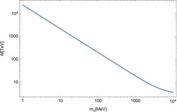
Figure 1: The magnetic dipole coupling scale $M=M_{d}/a_{m}$ as a function of dark matter mass $m_{\chi}$ in the range $1\,\mathrm{MeV}\leq m_{\chi}\leq 10\,\mathrm{GeV}$.

Since $M$ is related to the mass $m_{C}$ of a possible Kalb-Ramond field through $m_{C}=g_{BC}g_{C\chi}M$, coupling scales $M$ in the few TeV to thousands of TeV range could indicate a Kalb-Ramond mass in the hundreds of GeV to hundreds of TeV range if we assume weak strength couplings of the Kalb-Ramond field.

V Electron recoil cross section

As explained in the white paper rouven1 on new ideas in dark matter research, electron recoils are a primary possible signal for light dark matter particles with electromagnetic dipole moments.

The differential electron recoil cross section for the $U_{Y}(1)$ portal (25) in the lab frame and in the non-relativistic limit is for $m_{e}<m_{\chi}$ given by

$$\frac{d\sigma_{e}}{d\Omega} = \sum_{\pm}\frac{\alpha\cos^{2}\theta}{8\pi M^{2}}\frac{m_{e}m_{\chi}^{3}}{(m_{e}+m_{\chi})^{2}}\frac{1}{(\Delta\bm{k})_{\pm}^{2}}\!\left(1+\frac{9a_{e}^{2}}{2a_{m}^{2}}\right)$$ (31)

$$\times\frac{\left(\cos\varphi\pm\sqrt{(m_{e}/m_{\chi})^{2}-\sin^{2}\varphi}\right)^{2}}{\sqrt{(m_{e}/m_{\chi})^{2}-\sin^{2}\varphi}},$$

where $\varphi$ is the scattering angle between the incoming and scattered $\chi$ particle. The possible momentum transfers are in terms of the incoming $\chi$ momentum $\bm{k}$ and the scattering angle given by

$$\frac{(\Delta\bm{k})_{\pm}^{2}}{\bm{k}^{2}} = 1+\frac{\left(\cos\varphi\pm\sqrt{(m_{e}/m_{\chi})^{2}-\sin^{2}\varphi}\right)^{2}}{[1+(m_{e}/m_{\chi})]^{2}}$$ (32)

$$-\,2\cos\varphi\frac{\cos\varphi\pm\sqrt{(m_{e}/m_{\chi})^{2}-\sin^{2}\varphi}}{1+(m_{e}/m_{\chi})}.$$

The scattering angle is limited to

$$\varphi\leq\varphi_{max}=\arcsin(m_{e}/m_{\chi}).$$ (33)

The two branches in the scattering cross section arise from the fact that for $m_{e}<m_{\chi}$ there are two values of $|\bm{k}^{\prime}|/|\bm{k}|$ for every scattering angle $\varphi<\varphi_{max}$. The $(+)$ branch corresponds to an increase from $\varphi=0$ to $\varphi=\varphi_{max}$ with the scattered momentum $|\bm{k}^{\prime}|$ decreasing from $|\bm{k}^{\prime}|=|\bm{k}|$ to $|\bm{k}^{\prime}|=|\bm{k}|\sqrt{(m_{\chi}-m_{e})/(m_{\chi}+m_{e})}$. The $(-)$ branch corresponds to a subsequent decrease from $\varphi=\varphi_{max}$ to $\varphi=0$, with $|\bm{k}^{\prime}|$ further decreasing from $|\bm{k}^{\prime}|=|\bm{k}|\sqrt{(m_{\chi}-m_{e})/(m_{\chi}+m_{e})}$ to $|\bm{k}^{\prime}|=|\bm{k}|(m_{\chi}-m_{e})/(m_{\chi}+m_{e})$.

The dark matter abundance constraints in the previous section determine the magnetic coupling $M^{-1}=a_{m}/M_{d}$, but they do not determine $a_{e}/a_{m}$. Therefore we can only calculate the recoil cross section as a function of dark matter mass if we assume a ratio $(a_{e}/a_{m})^{2}$. Integration of $d\sigma_{e}/d\Omega$ yields electron recoil cross sections which are below the current limits from SuperCDMS cdms , XENON10/100 xenon , and SENSEI sensei , if $a^{2}_{e}<a^{2}_{m}$. This is displayed in Fig. 2, where $\beta_{\odot}=8.47\times 10^{-4}$ was used as a fiducial dark matter speed pdg .

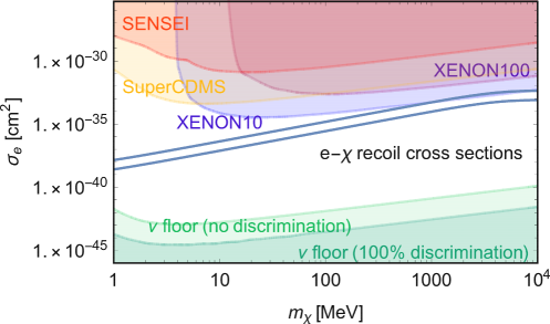
Figure 2: The electron recoil cross section as a function of dark matter mass $m_{\chi}$ in the range $1\,\mathrm{MeV}\leq m_{\chi}\leq 10\,\mathrm{GeV}$. The lower curve is for $a_{e}=0$ and the upper curve is for $a_{e}^{2}=a_{m}^{2}$. The neutrino floors with and without full separation of electron-neutrino and nucleon-neutrino scattering are taken from Ref. floor .

The recoil cross sections from a magnetic dipole coupling comply with the current direct exclusion limits throughout the considered mass range. On the other hand, the case $a_{e}=\pm a_{m}$ is excluded for masses in the GeV range. We also note that the recoil cross sections are above the neutrino floor floor and may be detectable with longer exposures or larger detectors.

VI Conclusions

Gauge invariant interactions of open strings require the Kalb-Ramond field to couple to the field strength tensors of $U(1)$ gauge fields, whereas a theory with only closed strings permits Cremmer-Scherk couplings to $U(1)$ field strength tensors. We found that these couplings can induce dipole couplings of electroweak singlet dark matter to the $U_{Y}(1)$ gauge field, thus contributing to the formation of a $U_{Y}(1)$ portal both to dark matter and to string theory. We analyzed in particular the case of a single dark matter component and found that the MeV-GeV mass range for dipole coupled dark matter remains viable under recent constraints from direct searches in electron recoils if $a_{e}^{2}<a_{m}^{2}$, while the case of dipole coupling only to right-handed or left-handed dark fermions $a_{e}=\pm a_{m}$ is excluded in the GeV mass rang but still allowed in the MeV mass range. Dipole coupled dark matter has a high discovery potential due to yielding recoil cross sections above the neutrino floor. The discovery of a dipole coupled $U_{Y}(1)$ portal to dark matter would therefore be very interesting from the perspective of a bottom-up approach to string phenomenology.

The model discussed here does not touch upon the important question of moduli stabilization, except for the observation that dilaton stabilization and an internal magnetic Kalb-Ramond flux decouple the Kalb-Ramond coupling in four dimensions from the mass term. We do assume that moduli are stabilized and that compactification yields the Standard Model at low energies. Our point is that under these circumstances the Kalb-Ramond field provides a natural candidate for inducing a dipole coupled $U_{Y}(1)$ portal to electroweak singlet dark matter. The discovery of $U_{Y}(1)$ dipole coupled dark matter would therefore provide an important low-energy indication for the existence of the anti-symmetric tensor fields of string theory.

- (1) M.W. Goodman, E. Witten, Detectability of certain dark matter candidates, Phys. Rev. D 31 (1985) 3059.
- (2) B. Patt, F. Wilczek, Higgs-field portal into hidden sectors, arXiv:hep-ph/0605188.
- (3) V. Silveira, A. Zee, Scalar Phantoms, Phys. Lett. B 161 (1985) 136.
- (4) J. McDonald, Gauge singlet scalars as cold dark matter, Phys. Rev. D 50 (1994) 3637.
- (5) M.C. Bento, O. Bertolami, R. Rosenfeld, L. Teodoro, Selfinteracting dark matter and invisibly decaying Higgs, Phys. Rev. D 62 (2000) 041302(R).
- (6) C. Burgess, M. Pospelov, T. ter Veldhuis, The Minimal Model of nonbaryonic dark matter: a singlet scalar, Nucl. Phys. B 619 (2001) 709.
- (7) H. Davoudiasl, R. Kitano, T. Li, H. Murayama, The new Minimal Standard Model, Phys. Lett. B 609 (2005) 117.
- (8) R. Schabinger, J.D. Wells, Minimal spontaneously broken hidden sector and its impact on Higgs boson physics at the CERN Large Hadron Collider, Phys. Rev. D 72 (2005) 093007.
- (9) C. Bird, R.V. Kowalewski, M. Pospelov, Dark matter pair-production in transitions, Mod. Phys. Lett. A 21 (2006) 457.
- (10) A. Djouadi, O. Lebedev, Y. Mambrini, J. Quevillon, Implications of LHC searches for Higgs-portal dark matter, Phys. Lett. B 709 (2012) 65.
- (11) R. Dick, Direct signals from electroweak singlets through the Higgs portal, Int. J. Mod. Phys. D 27 (2018) 1830008.
- (12) P. Athron et al. (GAMBIT Collaboration), Global analyses of Higgs portal singlet dark matter models using GAMBIT, Eur. Phys. J. C 79 (2019) 38.
- (13) K. Sigurdson, M. Doran, A. Kurylov, R.R. Caldwell, M. Kamionkowski, Dark-matter electric and magnetic dipole moments, Phys. Rev. D 70 (2004) 083501.
- (14) E. Masso, S. Mohanty, S. Rao, Dipolar dark matter, Phys. Rev. D 80 (2009) 036009.
- (15) V. Barger, W.-Y. Keung, D. Marfatia, Electromagnetic properties of dark matter: Dipole moments and charge form factor, Phys. Lett. B 696 (2011) 74.
- (16) J.H. Heo, Electric dipole moment of Dirac fermionic dark matter, Phys. Lett. B 702 (2011) 205.
- (17) J.-F. Fortin, T.M.P. Tait, Collider constraints on dipole-interacting dark matter, Phys. Rev. D 85 (2012) 063506.
- (18) J.M. Cline, G.D. Moore, A.R. Frey, Composite magnetic dark matter and the 130 GeV line, Phys. Rev. D 86 (2012) 115013.
- (19) J.H. Heo, C.S. Kim, Dipole-interacting fermionic dark matter in positron, antiproton, and gamma-ray channels, Phys. Rev. D 87 (2013) 013007.
- (20) S. Profumo, K. Sigurdson, Shadow of dark matter, Phys. Rev. D 75 (2007) 023521.
- (21) A.L. Fitzpatrick, K.M. Zurek, Dark moments and the DAMA-CoGeNT puzzle, Phys. Rev. D 82 (2010) 075004.
- (22) T. Banks, J.-F. Fortin, S. Thomas, Direct Detection of Dark Matter Electromagnetic Dipole Moments, arXiv:1007.5515 [hep-ph].
- (23) B. Feldstein, P.W. Graham, S. Rajendran, Luminous dark matter, Phys. Rev. D 82 (2010) 075019.
- (24) S. Chang, N. Weiner, I. Yavin, Magnetic inelastic dark matter, Phys. Rev. D 82 (2010) 125011.
- (25) J.P. Conlon, F. Day, N. Jennings, S. Krippendorf, M. Rummel, Consistency of Hitomi, XMM-Newton, and Chandra 3.5 keV data from Perseus, Phys. Rev. D 96 (2017) 123009.
- (26) M. Battaglieri et al., US Cosmic Visions: New Ideas in Dark Matter 2017: Community Report, arXiv:1707.04591 [hep-ph].
- (27) M.B. Green, J.H. Schwarz, E. Witten, Superstring Theory Vols. 1 & 2, Cambridge University Press, Cambridge (1987).
- (28) R. Blumenhagen, D. Lüst, S. Theisen, Basic Concepts of String Theory, Springer-Verlag, Berlin (2013).
- (29) M. Kalb, P. Ramond, Classical direct interstring action, Phys. Rev. D 9 (1974) 2273.
- (30) A. Chatterjee, P. Majumdar, Kalb-Ramond field interactions in a braneworld scenario, Phys. Rev. D 72 (2005) 066013.
- (31) J. Erdmenger, R. Meyer, J.P. Shock, AdS/CFT with flavour in electric and magnetic Kalb-Ramond fields, JHEP 0712 (2007) 091.
- (32) F.A. Barone, F.E. Barone, J.A. Helayël-Neto, Charged branes interactions via Kalb-Ramond field, Phys. Rev. D 84 (2011) 065026.
- (33) Yun-Zhi Du, Li Zhao, Yi Zhong, Chun-E Fu, Heng Guo, Resonances of Kalb-Ramond field on symmetric and asymmetric thick branes, Phys. Rev. D 88 (2013) 024009.
- (34) I.C. Jardim, G. Alencar, R.R. Landim, R.N. Costa Filho, Massive -form trapping as a -form on a brane, JHEP 1504 (2015) 003.
- (35) G. Alencar, I.C. Jardim, R.R. Landim, -Forms non-minimally coupled to gravity in Randall-Sundrum scenarios, Eur. Phys. J. C 78 (2018) 367.
- (36) R. Dick, Conformal gauge fixing in Minkowski space, Lett. Math. Phys. 18 (1989) 67.
- (37) J. Polchinski, A. Strominger, New vacua for type II string theory, Phys. Lett. B 388 (1996) 736.
- (38) J. Michelson, Compactifications of type IIB strings to four dimensions with non-trivial classical potential, Nucl. Phys. B 495 (1997) 127.
- (39) T.R. Taylor, C. Vafa, RR flux on Calabi-Yau and partial supersymmetry breaking, Phys. Lett. B 474 (2000) 130.
- (40) G. Curio, A. Klemm, D. Lüst, S. Theisen, On the vacuum structure of type-II string compactifications on Calabi-Yau spaces with H fluxes, Nucl. Phys. B 609 (2001) 3.
- (41) A.R. Frey, J. Polchinski, warped compactifications, Phys. Rev. D 65 (2002) 126009.
- (42) S. Kachru, R. Kallosh, A.D. Linde, S.P. Trivedi, de Sitter vacua in string theory, Phys. Rev. D 68 (2003) 046005.
- (43) Yeuk-Kwan E. Cheung, S. Watson, R. Brandenberger, Moduli stabilization with string gas and fluxes, JHEP 0605 (2006) 025.
- (44) I. Antoniadis, A. Kumar, T. Maillard, Magnetic fluxes and moduli stabilization, Nucl. Phys. B 767 (2007) 139.
- (45) V. Balasubramanian, P. Berglund, J.P. Conlon, F. Quevedo, Systematics of moduli stabilization in Calabi-Yau flux compactifications, JHEP 0503 (2005) 007.
- (46) M.R. Douglas, S. Kachru, Flux compactification, Rev. Mod. Phys. 79 (2007) 733.
- (47) I. Antoniadis, J.-P. Derendinger, T. Maillard, Nonlinear supersymmetry, effective actions and moduli stabilization, Nucl. Phys. B 808 (2009) 53.
- (48) B.S. Acharya, G. Kane, P. Kumar, Compactified string theories - generic predictions for particle physics, Int. J. Mod. Phys. A 27 (2012) 1230012.
- (49) F. Quevedo, Local string models and moduli stabilization, Mod. Phys. Lett. A 30 (2015) 1530004.
- (50) R. Blumenhagen, A. Font, M. Fuchs, D. Herschmann, E. Plauschinn, Y. Sekiguchi, F. Wolf, A flux-scaling scenario for high-scale moduli stabilization in string theory, Nucl. Phys. B 897 (2015) 500.
- (51) I. Antoniadis, Y. Chen, G.K. Leontaris, Perturbative moduli stabilization in type IIB/F-theory framework, Eur. Phys. J. C 78 (2018) 766.
- (52) W. Buchmuller, M. Dierigl, E. Dudas, Flux compactifications and naturalness, JHEP 1808 (2018) 151.
- (53) L.V. Avdeev, M.V. Chizhov, Antisymmetric tensor matter fields: An abelian model, Phys. Lett. B 321 (1994) 212.
- (54) V. Lemes, R. Renan, S.P. Sorella, Algebraic renormalization of antisymmetric tensor matter fields, Phys. Lett. B 344 (1995) 158.
- (55) V. Lemes, R. Renan, S.P. Sorella, Renormalization of nonabelian gauge theories with tensor matter fields, Phys. Lett. B 392 (1997) 106.
- (56) E. Cremmer, J. Scherk, Spontaneous dynamical breaking of gauge symmetry in dual models, Nucl. Phys. B 72 (1974) 117.
- (57) P. Gondolo, G. Gelmini, Cosmic abundances of stable particles: Improved analysis, Nucl. Phys. B 360 (1991) 145.
- (58) B.W. Lee, S. Weinberg, Cosmological lower bound on heavy-neutrino masses, Phys. Rev. Lett. 39 (1977) 165.
- (59) E.W. Kolb, M.S. Turner, The Early Universe, Westview Press, Boulder (1994).
- (60) S. Dodelson, Modern Cosmology, Academic Press, San Diego (2003).
- (61) R. Agnese et al. (SuperCDMS Collaboration), First dark matter constraints from a SuperCDMS single-charge sensitive detector, Phys. Rev. Lett. 121 (2018) 051301.
- (62) R. Essig, T. Volansky, T.-T. Wu, New constraints and prospects for sub-GeV dark matter scattering off electrons in xenon, Phys. Rev. D 96 (2017) 043017.
- (63) M. Crisler et al. (SENSEI Collaboration), SENSEI: First direct-detection constraints on sub-GeV dark matter from a surface run, Phys. Rev. Lett. 121 (2018) 061803.
- (64) M. Tanabashi et al. (Particle Data Group), Review of Particle Physics, Phys. Rev. D 98 (2018) 030001.
- (65) J. Wyenberg, I.M. Shoemaker, Mapping the neutrino floor for direct detection experiments based on dark matter-electron scattering, Phys. Rev. D 97 (2018) 115026.