Production of pions, kaons and protons in Xe–Xe collisions at $\mathbf{\sqrt{{\textit{s}}_{\mathbf{\rm\mathbf{NN}}}}=5.44}\text{ TeV}$

Abstract:

In late 2017, the ALICE experiment recorded a data sample of Xe–Xe collisions at the unprecedented energy in A–A systems of $\sqrt{s_{\rm{NN}}}=5.44\text{ TeV}$. The $p_{\rm T}$ spectra at mid-rapidity ($|y|<0.5$) of pions, kaons and protons are presented. The preliminary $p_{\rm T}$ spectra are obtained by combining independent analyses with the Inner Tracking System (ITS), the Time Projection Chamber (TPC), and the Time-Of-Flight (TOF) detectors. This paper focuses on the details of the analysis performed with TOF and in particular on the performance implications of the special Xe–Xe run conditions. The peculiarity of this data set comes from the experimental conditions: because of the lower magnetic field of the ALICE solenoid ($B=0.2\text{ T}$, lower than the nominal $0.5\text{ T}$) we expect to explore a $p_{\rm T}$ region unattainable before. A comparison between the yields at different centrality bins will also be provided.

1 Introduction

The ALICE Collaboration has built a dedicated heavy-ion collisions detector to investigate a new state of matter, the QGP (Quark–Gluon Plasma), which is expected to be created in these collisions. One way to quantify the expansion velocity of the system produced in heavy-ion collisions is to study the production of identified particles, particularly their transverse momentum distributions. The final-state distributions are governed by the temperature at which the system freezes out and the particles no longer interact. If the values of the temperature agree for different particle species, e.g. pions, kaons, protons, and antiprotons, this indicates a global freeze-out temperature and fluid velocity. While the low-$p_{\rm T}$ end of the spectrum involves particles which are more likely to be in thermal equilibrium, the high-$p_{\rm T}$ particles are more likely to have been produced in hard scatterings, governed by perturbative QCD.

Ultimately, this study addresses the question whether the matter reaches kinetic equilibrium. If we suppose that the system created in heavy-ion collisions is in kinetic equilibrium, the pressure is built inside the system. The matter is surrounded by vacuum, so a pressure gradient in outward directions generates collective flow and, in turn, the system expands radially. When the matter is moving at a finite velocity the momentum distribution is Lorentz boosted and the magnitude of this boost is proportional to the particle mass. If this kind of effect in the momentum distribution can be observed experimentally, one can obtain some information about kinetic equilibrium. Assuming each fluid element expands radially at a radial flow velocity $\beta_{\rm T}$ , the $p_{\rm T}$ spectra for pions and protons can be calculated by convoluting these affected momentum distributions over the azimuthal direction, which is realized in the blast wave model [1, 2].

2 Analysis procedure

The measurement of the production of $\pi^{\pm}$, K^±, p and $\bar{\text{p}}$ in Xe–Xe collisions at $\sqrt{s_{\rm NN}}=5.44\text{ TeV}$ has been performed for ITS, TPC and TOF [3] separately, but in the following we will focus on the TOF analysis only.

The final goal is the combination of all individual analyses so as to provide a single spectrum covering the widest $p_{\rm T}$ interval possible with the best precision, combined results are shown in Sec. 3. The final spectra represent the combination of the three individual analyses. The $p_{\rm T}$-ranges of the different analyses are given in Tab. 1.

Analysis	$\pi$	K	p
ITSsa	0.08-0.70 GeV$/$c	0.20-0.45 GeV$/$c	0.30-0.50 GeV$/$c
TOF	0.40-5.00 GeV$/$c	0.4-3.60 GeV$/$c	0.50-5.00 GeV$/$c
TPC	0.25-0.70 GeV$/$c	0.25-0.45 GeV$/$c	0.40-0.80 GeV$/$c

Table 1: $\pi$, K and p $p_{\rm T}$ ranges in GeV$/$c used for the different detectors in the analysis of Xe–Xe collisions.

2.1 TOF analysis

The analysis relies on the global tracks and the extraction of the total yield by performing particle identification (PID) exclusively with the TOF detector. The main goal of this analysis is to provide spectra as a function of $p_{\rm T}$ for identified $\pi^{+}$, $\pi^{-}$, K⁺, K^-, p and $\bar{\text{p}}$ at intermediate $p_{\rm T}$, which are then combined with the ITS and TPC spectra. The strategy, as it will be better explained in the following, is based on the comparison between the measured time of flight and the theoretical prediction for each mass hypothesis.

The analysis strategy mainly relies on tracks reconstructed in the TPC, which are extrapolated to the TOF. The assignment of a TOF cluster to the propagated track allows one to use the precise measurement of the arrival time of the particle at the TOF surface. Examples of the measured particle velocity can be seen in Fig. 1(a) for Xe–Xe collisions.

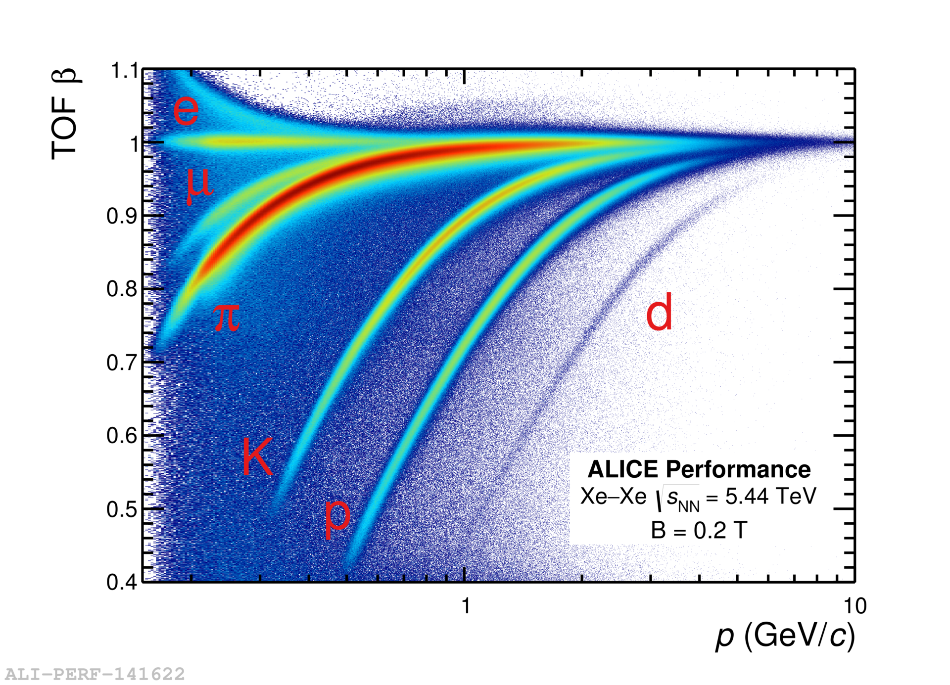
(a) Beta vs $p$ measured with the TOF detector.

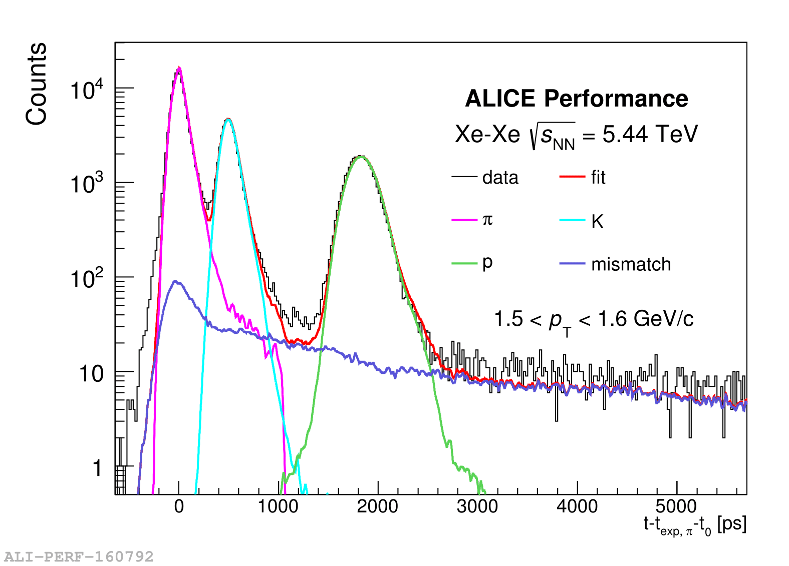
(b) TOF signal: single template components.

Figure 1: Left panel: beta measured with the TOF detector as a function of the track momentum in Xe–Xe collisions at $\sqrt{s_{\rm NN}}=5.44\text{ TeV}$. The visible bands are from $e$, $\mu$, $\pi$, K, p and d. The contribution from wrongly associated tracks can be seen outside the bands. Right panel: the TOF signal fit with single template components. The mismatch is depicted with a dark blue color, pions with magenta, kaons with light blue and protons with green.

The identification of different particle types is performed with a statistical approach, measuring the time-of-flight as

$$time\text{-}of\text{-}flight=T_{\rm TOF}-T_{\rm 0}\text{ .}$$ (1)

The time of flight is defined as the difference between the time measured by the TOF detector and the start time $T_{\rm 0}$. For simplicity from now on we will refer to the $time\text{-}of\text{-}flight$ as $t$.

The expected time-of-flight ($t_{\rm exp,\text{\it i}}$) can be numerically computed for every particle species i for each track by taking into account the track length and the energy loss in the material.

The PID strategy with TOF takes advantage of the separation between the different particles by calculating the $n\sigma$ separation

$$n\sigma_{i}=\frac{t-t_{{\rm exp,}i}}{\sigma_{i}}\text{ ,}$$ (2)

indicating by $n\sigma_{i}$ the distance in number of sigmas of the measured value from the expected one under a specific mass hypothesis, and by $\sigma_{i}$ the uncertainty on the numerator. The uncertainty $\sigma_{i}$ can be expressed as $\sigma_{i}^{2}=\sigma_{\rm TOF}^{2}+\sigma_{T_{\rm 0}}^{2}+\sigma_{t_{\rm exp}}^{2}$ which are the intrinsic contribution due to the TOF itself, the resolution of the start time of the event, and the contribution due to the expected time of flight for a certain particle species, respectively.

The $T_{0}$ can be determined with different methods [4], each with different precision. The measurement of the $T_{0}$ with the TOF is fully efficient in Xe–Xe collisions from central collisions up to centrality bin $80$–$90\%$, where the multiplicity of tracks reaching the TOF is not high enough to ensure the determination of the event time in each collision. In this case, the measurement of the start time relies mostly on the T0 detector or, in case it is not available, on the nominal bunch crossing time, which results in a worse time-of-flight resolution.

2.2 TOF signal

The signal in the TOF detector must be correctly parametrized to perform the particle identification. The parameterization is given by

$$f(t)=\begin{cases}A\cdot\textit{Gaus}(t,\mu,\sigma),&\textit{if $t\leq\mu+\tau$}.\\ A\cdot\textit{Gaus}(\mu+\tau,\mu,\sigma)\cdot\exp\left[-\frac{\tau\cdot\left(t-\mu-\tau\right)}{\sigma^{2}}\right],&\textit{otherwise}.\end{cases}$$ (3)

where $A$ is a normalization factor. Basically the actual form of $f(t)$ is a Gaussian distribution with an exponential tail on the right side of the peak, see Fig. 2(a).

The parameters are tuned on experimental data and are set to $\mu=0$ and $\tau=0.85\sigma$. These parameters are intrinsic to the TOF detector and are to be taken as asymptotic values that are measured once the particle momentum is high enough that the energy loss becomes negligible. The parameters used to describe the TOF signal are extracted with a fit to the distribution of $t-t_{\rm exp,\pi}-t_{\rm 0}$ in the region where the peak for $\pi$ is clearly separated in TOF.

(a) TOF signal.

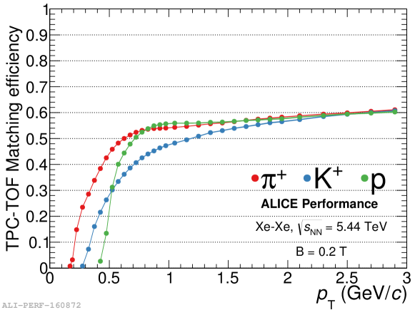
(b) Matching efficiency.

Figure 2: The TOF signal (upper panel) and the matching efficiency for pions, kaons, and protons (lower panel).

The raw spectra extracted in this way have to be corrected for the presence of secondary particles, for the tracking efficiency, and the matching efficiency (see Fig. 2(b)), before they can undergo combinations with spectra from ITS and TPC.

3 Results

The combined spectra are shown on Fig. 3(a), 3(b), and 3(c). It is evident that they show all the features expected from radial flow: the spectra get harder with increasing mass of the particle of interest, e.g. going from pions to protons, and the spectra get harder with increasing centrality (most evident for the proton spectra). The $p_{\rm T}$ spectra here shown, may be then fitted with a Blast-Wave parameterization, in order to extract the kinetic freeze-out temperature and the radial flow velocity. Subsequently, the values obtained for Xe–Xe collisions, may be compared with those obtained for Pb–Pb collisions at $\sqrt{s_{\rm NN}}=2.76\text{, }5.02\text{ TeV}$.

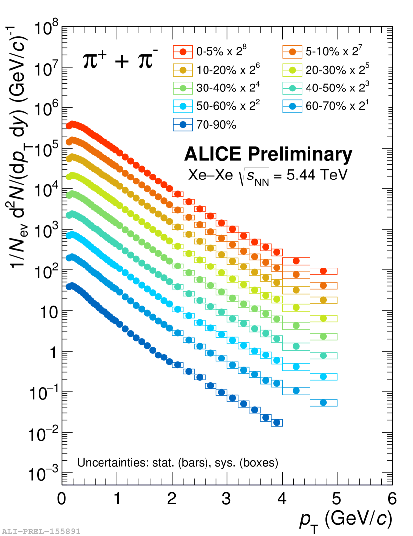
(a) Combined spectra for $\pi$.

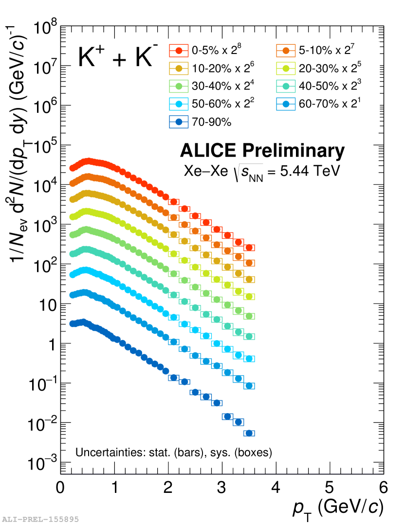
(b) Combined spectra for K.

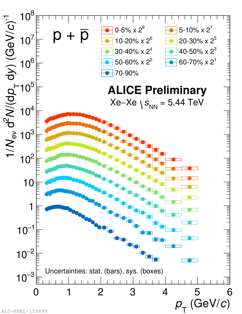
(c) Combined spectra for p.

Figure 3: Combined spectra for $\pi$, K and p for all the centrality classes considered in Xe–Xe collisions at $\sqrt{s_{\rm NN}}=5.44\text{ TeV}$.

References

- [1] P.J. Siemens and J.O. Rasmussen: Phys. Rev. Lett. 42, 880 (1979) 157, 158.
- [2] E. Schnedermann, J. Sollfrank and U.W. Heinz: Phys. Rev. C 48, 2462 (1993) 157, 158.
- [3] B. Abelev et al. (ALICE Collaboration), Int. J. Mod. Phys. A29 (2014) 1430044.
- [4] J. Adam et al. (ALICE Collaboration), Eur. Phys. J. Plus 132 (2017) no.2, 99.