SchNetPack: A Deep Learning Toolbox For Atomistic Systems

Abstract

SchNetPack is a toolbox for the development and application of deep neural networks to the prediction of potential energy surfaces and other quantum-chemical properties of molecules and materials. It contains basic building blocks of atomistic neural networks, manages their training and provides simple access to common benchmark datasets. This allows for an easy implementation and evaluation of new models. For now, SchNetPack includes implementations of (weighted) atom-centered symmetry functions and the deep tensor neural network SchNet as well as ready-to-use scripts that allow to train these models on molecule and material datasets. Based upon the PyTorch deep learning framework, SchNetPack allows to efficiently apply the neural networks to large datasets with millions of reference calculations as well as parallelize the model across multiple GPUs. Finally, SchNetPack provides an interface to the Atomic Simulation Environment in order to make trained models easily accessible to researchers that are not yet familiar with neural networks.

I Introduction

One of the fundamental aims of modern quantum chemistry, condensed matter physics and materials science is to numerically determine the properties of molecules and materials. Unfortunately, the computational cost of accurate calculations prove prohibitive when it comes to large-scale molecular dynamics simulations or the exhaustive exploration of the vast chemical space. Over the last years however, it has become clear that machine learning is able to provide accurate predictions of chemical properties at significantly reduced computational costs. Conceptually, this is achieved by training a machine learning model to reproduce the results of reference calculations given the configuration of an atomistic system. Once trained, predicting properties of other atomistic systems is generically cheap and has been shown to be sufficiently accurate for a range of applications bartok2010gaussian; rupp2012fast; schutt2014represent; behler2015constructing; huo2017unified; faber2018alchemical; de2016comparing; morawietz2016van; gastegger2017machine; chmiela2017machine; faber2017prediction; podryabinkin2017active; brockherde2017bypassing; bartok2017machine; schutt2018schnet; chmiela2018towards; ziletti2018insightful; dragoni2018achieving.

A common subclass of machine learning models for quantum-chemistry are atomistic neural networks. There exist various architectures of these models, which can be broadly split into two categories: descriptor-based models that take a predefined representation of the atomistic system as input behler2007generalized; montavon2012learning; montavon2013machine; zhang2018deep; smith2017ani; gastegger2018wacsf and end-to-end architectures that learn a representation directly from atom types and positions schuett2017quantum; gilmer2017neural; schutt2017schnet; lubbers2018hierarchical.

SchNetPack provides a unified framework for both categories of neural networks. While we plan to support more architectures in the future, SchNetPack currently includes implementations for SchNet schutt2017schnet; schutt2018schnet, an end-to-end continuous convolution architecture, as well as Behler–Parrinello networks which are based on atom-centered symmetry functions (ACSF) behler2007generalized; behler2011atom and an extension thereof which uses weighted atom-centered symmetry functions (wACSF) gastegger2018wacsf.

SchNetPack furthermore contains functionality for accessing popular benchmark datasets, training neural networks on (multiple) GPUs to predict a variety of chemical properties. It is built in an extensible manner and is implemented using the PyTorch deep learning framework.

The remainder of the paper is structured as follows. In Section II, we present how models in SchNetPack are structured and briefly review (w)ACSF and SchNet representations. Section II.2 outlines how SchNetPack manages the training process for atomistic neural networks and gives an overview of the integrated datasets. Section LABEL:sec:implementation summarizes details about the implementation, while Sections LABEL:sec:example and LABEL:sec:spkfc provide code examples for training an atomistic neural network and calculating a power spectrum using the interface to the Atomic Simulation Environment (ASE). Section LABEL:sec:results presents results of SchNetPack on standard benchmarks, before we conclude and give an outlook on future extensions.

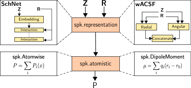
Figure 1: Basic building blocks of a model predicting the property $P$ from the positions $R$ and atomic numbers $\mathbf{Z}$ of the atomistic system. We use the abbreviation ${\verb{}{}\@hidden@egroup spk${}{}\@hidden@egroup spkforthe$\verb{}{}\@hidden@egroup schnetpack${}{}\@hidden@egroup schnetpackpackage.All\textit{representation}and\textit{prediction}blocksarecollectedinthe$\verb{}{}\@hidden@egroup spk.representation${}{}\@hidden@egroup spk.representationand$\verb{}{}\@hidden@egroup spk.atomistic${}{}\@hidden@egroup spk.atomisticpackagerespectively.Therightandleftpanelsillustratevariouschoicesforthesebuildingblocks.}$

II Models

Models in SchNetPack have two principle components: representation and prediction blocks (see Figure I). The former takes the configuration of the atomistic system as an input and generates feature vectors describing each atom in its chemical environment. The latter uses these atom-wise representations to predict the desired properties of the atomistic system. The only difference between descriptor-based and end-to-end architectures is whether the representation block is fixed or learned from data. In the following two sections, we will explain the possible choices for these components in detail.

II.1 Representations

An atomistic system containing $n$ atoms can be described by its atomic numbers $\mathbf{Z}=(Z_{1},\dots,Z_{n})$ and positions $R=(\mathbf{r}_{1},\dots,\mathbf{r}_{n})$. The interatomic distances are given as $r_{ij}=\left\lVert\mathbf{r}_{i}-\mathbf{r}_{j}\right\rVert$. In the following, we will briefly describe the currently implemented representations, i.e. (w)ACSF gastegger2018wacsf and SchNet schutt2017schnet. For further details, refer to the original publications.

II.1.1 (w)ACSF

Behler--Parrinello network potentials behler2007generalized have proven very useful for systems as diverse as small molecules, metal and molecular clusters, bulk materials, surfaces, water and solid-liquid interfaces (for a recent review, see behler2017first). Due to this impressive number of applications, Behler--Parrinello networks are now firmly established as a highly successful neural network architecture for atomistic systems.

For these networks, so-called atom-centered symmetry functions (ACSFs) form the representation of the atomistic system. Contrary to the approach taken by SchNet, where features are learned from the data, ACSFs need to be determined before training. Hence, using symmetry functions can be advantageous in situations where the available training data is insufficient to learn suitable representations in an end-to-end fashion. On the other hand, introducing rigid hand-crafted features might reduce the generality of the model. In the following, we will briefly review ACSFs and a variant called weighted ACSFs, or wACSFs for short. We refer to References behler2011atom and gastegger2018wacsf for a more detailed discussion.

ACSFs describe the local chemical environment around a central atom via a combination of radial and angular distribution functions.

Radial Symmetry Functions:

Radial ACSF descriptors take the form:

$$G_{i,\alpha}^{rad}=\sum_{j\neq i}^{N}g(Z_{j})e^{-\gamma_{\alpha}(r_{ij}-\mu_{\alpha})^{2}}f(r_{ij}),$$ (1)

where $i$ is the central atom and the sum runs over all neighboring atoms $j$. $\gamma_{\alpha}$ and $\mu_{\alpha}$ are parameters which modulate the widths and centers of the Gaussians. Typically, a set of $n_{\mathrm{rad}}$ radial symmetry functions with different parameter combinations $\alpha\in\{1,\dots,n_{\mathrm{rad}}\}$ are used. In SchNetPack, suitable $\gamma_{\alpha}$ and $\mu_{\alpha}$ are determined automatically via an equidistant grid between zero and a spacial cutoff $r_{c}$, adopting the empirical parametrization strategy detailed in Reference gastegger2018wacsf.

A cutoff function $f$ ensures that only atoms close to the central atom $i$ enter the sum and is given by

$$f(r_{ij})=\begin{cases}\tfrac{1}{2}\left(\cos(\tfrac{\pi r_{ij}}{r_{c}})+1\right)\,,&r_{ij}\leq r_{c}\,,\\ 0\,,&\,\text{else}\,.\end{cases}$$ (2)

For convenience, we will use the notation $f_{ij}=f(r_{ij})$ in the following. Finally, $g(Z_{j})$ is an element-dependent weighting function. In ACSFs, $g(Z_{j})$ takes the form

$$g(Z_{j})=\delta_{Z_{j},Z_{\mathfrak{a}}}=\begin{cases}1&\mbox{if }Z_{j}=Z_{\mathfrak{a}}\\ 0&\mbox{else}.\end{cases}$$ (3)

Hence, radial ACSFs are always defined between the central atom and a neighbor belonging to a specific chemical element.

Angular Symmetry Functions:

information about the angles between atoms are encoded by the $n_{a}$ angular symmetry functions

$$G_{i,\alpha}^{ang}= 2^{1-\zeta_{\alpha}}\sum^{N}_{j\neq i,k>j}g(Z_{j},Z_{k})\left(1+\lambda\theta_{ijk}\right)^{\zeta_{\alpha}}\,$$

$$\times e^{-\gamma_{\alpha}\left(r_{ij}^{2}+r_{ik}^{2}+r_{jk}^{2}\right)}f_{ij}\,f_{ik}\,f_{jk}\,,$$ (4)

where $\theta_{ijk}$ is the angle spanned between atoms $i$, $j$ and $k$. The parameter $\lambda$ takes the values $\lambda=\pm 1$ which shifts the maximum of the angular terms between $0$ and $\pi$. The variable $\zeta_{\alpha}$ is a hyperparameter controlling the width around this maximum. $\gamma_{\alpha}$ once again controls the width of the Gaussian functions. As with radial ACSFs, a set of $n_{\mathrm{ang}}$ angular functions differing in their parametrization patterns $\alpha\in\{1,\dots,n_{\mathrm{ang}}\}$ is chosen to describe the local environment. For angular ACSFs, the weighting function $g(Z_{k},Z_{j})$ can be expressed as

$$g(Z_{k},Z_{j})=\frac{1}{2}\left(\delta_{Z_{j}Z_{\mathfrak{a}}}\delta_{Z_{k}Z_{\mathfrak{b}}}+\delta_{Z_{j}Z_{\mathfrak{b}}}\delta_{Z_{k}Z_{\mathfrak{a}}}\right),$$ (5)

which counts the contributions of neighboring atoms $j$ and $k$ belonging to a specific pair of elements (e.g. O-H or O-O).

Due to the choice of $g$, ACSFs always are defined for pairs (radial) or triples (angular) of elements and at least one parametrized function $G_{\mathrm{i,\alpha}}$ has to be provided for each of these combinations. As a consequence, the number of ACSFs grows quadratically with the number of different chemical species. This can lead to an impractical number of ACSFs for systems containing more than four elements (e.g. QM9).

Recently, alternative weighting functions have been proposed which circumvent the above issue. In these so-called weighted ACSFs (wACSFs), the radial weighting function is chosen as $g(Z_{j})=Z_{j}$ while the angular function is set to $g(Z_{k},Z_{j})=Z_{k}Z_{j}$. Through this simple reparametrization, the number of required symmetry functions becomes independent of the actual number of elements present in the system, leading to more compact descriptors. SchNetPack uses wACSFs as the standard descriptor for Behler--Parrinello potentials.

Irrespective of the choice for the weighing $g$, both radial and angular symmetry functions are concatenated as a final step to form the representation for the atomistic system, i.e.

$$X_{i}=\left(G^{rad}_{i,1},\dots G^{rad}_{i,n_{\mathrm{rad}}},G^{ang}_{i,1}|_{\lambda=\pm 1},\dots,,G^{ang}_{i,n_{\mathrm{ang}}}|_{\lambda=\pm 1}\right)\,.$$ (6)

This representation $X_{i}$ can then serve as input for prediction block of the atomistic network.

II.1.2 SchNet

SchNet is an end-to-end deep neural network architecture based on continuous-filter convolutions schutt2017schnet; schutt2018schnet. It follows the deep tensor neural network framework schuett2017quantum, i.e. atom-wise representations are constructed by starting from embedding vectors that characterize the atom type before introducing the configuration of the system by a series of interaction blocks.

Convolutional layers in deep learning usually act on discretized signals such as images. Continuous-filter convolutions are a generalization thereof for input signals that are not aligned on a grid, such as atoms at arbitrary positions. Contrary to (w)ACSF networks which are based on rigid hand-crafted features, SchNet adapts the representation of the atomistic system to the training data. More precisely, SchNet is a multi-layer neural network which consists of an embedding layer and several interaction blocks, as shown in the top left panel of Figure I. We describe its components in more detail in the following:

Atom Embeddings:

Using an embedding layer, each atom type $Z_{i}$ is represented by feature vectors $\mathbf{x}^{0}_{i}\in\mathbb{R}^{F}$ which we collect in a matrix $X^{0}=(\mathbf{x}^{0}_{1},\dots,\mathbf{x}^{0}_{n})$. The feature dimension is denoted by $F$. The embedding layer is initialized randomly and adapted during training. In all other layers of SchNet, atoms are described analogously and we denote the features of layer $l$ by $X^{l}=(\mathbf{x}^{l}_{1},\dots,\mathbf{x}^{l}_{n})$ with $\mathbf{x}^{l}_{i}\in\mathbb{R}^{F}$.

Interaction Blocks:

Using the features $X^{l}$ and positions $R$, this building block computes interactions which additively refine the previous representation analogue to ResNet blocks he2016deep. To incorporate the influence of neighboring atoms, continuous-filter convolutions are applied which are defined as follows:

$$\mathbf{x}_{i}^{l+1}=(X^{l}*W^{l})\equiv\sum_{j\in\text{nbh}(i)}\mathbf{x}_{j}^{l}\odot W^{l}(r_{ij})\,.$$ (7)

By $\odot$ we denote element-wise multiplication and $\text{nbh}(i)$ are the neighbors of atom $i$. In particular for larger systems, it is recommended to introduce a radial cutoff. For our experiments, we use a distance cutoff of 5Å.

Here, the filter is not a parameter tensor as in standard convolutional layers, but a filter-generating neural network $W^{l}:\mathbb{R}\to\mathbb{R}^{F}$ which maps atomic distances to filter values. The filter generator takes atom positions expanded on a grid of radial basis functions which are closely related to the radial symmetry functions (1) of (w)ACSF. For its precise architecture, we refer to the original publications schutt2017schnet; schutt2018schnet.

Several atom-wise layers, i.e. fully-connected layers

$$\mathbf{x}^{l+1}_{i}=W^{l}\mathbf{x}^{l}_{i}+\mathbf{b}^{l}\,$$ (8)

that are applied to each atom $i$ separately, recombine the features within each atom representation. Note that the weights $W^{l}$ and biases $\mathbf{b}^{l}$ are independent of $i$ and are therefore the same for all atom features $\mathbf{x}^{l}_{i}$. Thus the number of parameters of atom-wise layers is independent of the number of atoms $n$.

In summary, SchNet obtains a latent representation of the atomistic system by first using an embedding layer to obtain features $X^{0}$. These features are then processed by $L$ interaction blocks which results in the latent representation $X^{L}$ which can be passed to the prediction block. We will sketch the possibilities for the architectures of these prediction blocks in the following section.

II.2 Prediction Blocks

As discussed in the last sections, both SchNet and (w)ACSF provide representations $X_{i}$ with $i\in\{1,\dots,n\}$ for an atomistic system with $n$ atoms. These representations are then processed by a prediction block to obtain the desired properties of the atomistic system. There are various choices for prediction blocks depending on the property of interest. Usually, prediction blocks consist of several atom-wise layers (8) with non-linearities, which reduce the feature dimension, followed by a property-dependent aggregation across atoms.

The most common choice are

Atomwise} prediction blocks, which express a desired molecular property $P$ as a sum of atom-wise contributions
\begin

alignP=∑i=1np(xi). While this is a suitable model for extensive properties such as the energy, intensive properties, which do not grow with the number of atoms $n$ of the atomistic system, are instead expressed as the average over contributions.

Atomwise} prediction blocks are suitable for many properties, however property-specific prediction blocks may be used to incorporate prior knowledge into the model.
The \mintinline

pythonDipoleMoment prediction block expresses the dipole moment $\mathbf{\mu}$ as

$$\mathbf{\mu}=\sum_{i=1}^{n}q(\mathbf{x}_{i})(\mathbf{r}_{i}-\mathbf{r}_{0})\,,$$ (9)

where $q:\mathbb{R}^{F}\to\mathbb{R}$ can be interpreted as latent atomic charges and $\mathbf{r}_{0}$ denotes the center of mass of the system.

The ElementalAtomwise} prediction block is different from \mintinlinepythonAtomwise in that instead of applying the same network to all the atom features $X_{i}$, it uses separate networks for different chemical elements. This is particularly useful for (w)ACSF representations. Analogously,

ElementalDipoleMoment} is defined for the dipole moment.
\section

Data Pipeline and Training

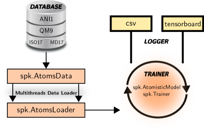
Figure 2: Setup for training models in SchNetPack. Note that we denote the various choices for dataset classes mentioned in Section II.2 by their common base class.

One of the main aims of SchNetPack is to accelerate the development and application of atomistic neural networks. To this end, SchNetPack contains a number of classes which provide access to standard benchmark datasets and manage the training process. Figure II.2 summarizes this.

The dataset classes automatically download the relevant data, if not already present on disk, and use the standard ASE package ase to store them in an SQLite database. In particular, this means that we use the conventions and units of the ASE package in SchNetPack, e.g. energies and lengths are in units of $\mathrm{eV}$ and $\mathrm{\SIUnitSymbolAngstrom}$. Currently, SchNetPack includes the following dataset classes:

• schnetpack.datasets.QM9}: class for the QM9 dataset~\citeqm9one,qm9two

for 133,885 organic molecules with up to nine heavy atoms from $\ce{C}$, $\ce{O}$, $\ce{N}$ and $\ce{F}$.

schnetpack.datasets.ANI1}: functionality to access ANI-1 dataset~\citeani1 which consists of more than 20 million conformations for 57454 small organic molecules from $\ce{C}$, $\ce{O}$ and $\ce{N}$.

schnetpack.datasets.ISO17}: class for ISO17 dataset~\citeqm9two, schutt2017schnet, schuett2017quantum

for molecular dynamics of $\ce{C_{7}O_{2}H_{10}}$ isomers. It contains 129 isomers with 5000 conformational geometries and their corresponding energies and forces.

schnetpack.datasets.MD17}: class for MD17 dataset~\citechmiela2017machine, schuett2017quantum for molecular dynamics of small molecules containing molecular forces.

schnetpack.datasets.MaterialsProject}: provides access to the Materials Project~\citemp1repositoryofbulkcrystalcontainingatomtypesrangingacrossthewholeper