Group-Representative Functional Network Estimation from Multi-Subject fMRI Data via MRF-based Image Segmentation

Abstract

We propose a novel two-phase approach to functional network estimation of multi-subject functional Magnetic Resonance Imaging (fMRI) data, which applies model-based image segmentation to determine a group-representative connectivity map. In our approach, we first improve clustering-based Independent Component Analysis (ICA) to generate maps of components occurring consistently across subjects, and then estimate the group-representative map through MAP-MRF (Maximum a priori - Markov random field) labeling. For the latter, we provide a novel and efficient variational Bayes algorithm. We study the performance of the proposed method using synthesized data following a theoretical model, and demonstrate its viability in blind extraction of group-representative functional networks using simulated fMRI data. We anticipate the proposed method will be applied in identifying common neuronal characteristics in a population, and could be further extended to real-world clinical diagnosis.

1 Introduction

fMRI systems capture neuronal activity by imaging the accompanying changes in blood flow. Increased activity demands greater energy, which triggers increased local blood flow and oxygenation (Matthews, 2003). Further, differences in magnetic properties of oxyhaemoglobin (diamagnetic) and deoxyhaemoglobin (paramagnetic) enable us to record the level of neuronal activity under an applied magnetic field, as a function of the deoxyhaemoglobin content of blood (Huettel et al., 2004). fMRI systems are noninvasive with high spatial and temporal resolution, leading to their popularity as tools for identification of brain regions that are active in tandem, referred to as functionally connected networks.

There has been growing interest in using functional connectivity patterns, determined from fMRI data, to characterize groups of individuals exhibiting common traits. Applications include identifying individuals with neurological and psychiatric diseases on the basis of observed abnormalities in functional connectivity (Fox and Greicius, 2010). Recent work analyzing clinical data of patients with neurological diseases, such as Alzheimer’s (Greicius et al., 2004), epilepsy (Xu et al., 2013), and multiple sclerosis (Au Duong et al., 2005), demonstrates the strong potential of fMRI as a diagnostic tool in clinical practice. However, the present challenge lies in efficient and accurate identification of distinct functional connectivity patterns observed consistently across multiple subjects (Cole et al., 2010).

Functional networks of individual subjects have been successfully uncovered from their fMRI data through independent components analysis (ICA, Mckeown et al., 1998). ICA is a technique that separates individual source components from a linear mixture, under assumptions of independence and non-Gaussianity (Hyvärinen et al., 2004). For the identification of connectivity patterns across multiple subjects, several extensions of single-subject ICA have been proposed, primarily involving data aggregation through across-subject averaging (Schmithorst and Holland, 2004), data concatenation (Calhoun et al., 2001a), and clustering-based schemes (Esposito et al., 2005). While across-subject averaging reduces computation, it requires perfect registration across subjects; leading to loss of sensitivity due to suppression of unique and minority sources, as well as loss of resolution (Esposito et al., 2005). Concatenation-based methods make the imposition of a common observation space (for temporal concatenation) or common time course (for spatial concatenation) (Erhardt et al., 2011). While these methods are intended to prevent overfitting (Yeo and Ou, 2004), only a single spatial map or time course is attainable, applying to all subjects.

The third ICA scheme is the so-called self-organized clustering-based ICA (SOG-ICA, Esposito et al. (2005)). This two-stage procedure applies spatial ICA to individual subject data, followed by across-subject clustering to identify independent components that occur consistently. Cluster centroids are used to form the group-representative map. This has the advantage of allowing for differences between individual subject (spatial) maps and time courses, and for incorporation of both spatial and temporal similarities in measuring across-group consistency. However, the similarity measures recommended in Esposito et al. (2005) limit dimensionality reduction during pre-processing, and do not make allowance for minor relative shifts which may be reasonably expected between maps of different subjects. Additionally, the use of cluster centroids may yield incorrect results, as the averaged series may not belong to the valid space of fMRI signals (Yeo and Ou, 2004).

In this paper, we propose an alternative framework that redefines the problem of estimating the group map as an image segmentation problem. We first employ an improved clustering-based ICA scheme, incorporating spatial and temporal similarity measures that accommodate for minor shifts between subjects, to determine consistent components underlying individual subject maps. Our main contribution is then an MAP-MRF framework that models this data, as well as a novel and efficient variational Bayes algorithm Wainwright and Jordan (2003) to identify distinct functional networks across the subjects. Our framework exploits spatial information underlying the connectivity maps, and accounts for uncertainty in the estimation process, overcoming limitations in more traditional schemes.

The remainder of this paper is organized as follows. In Section 2, we describe our problem in more detail, and the pre-processing steps. In Section 3, we specify the various components of our modeling framework, as well as the details of our proposed computational framework. In Section 4, we specify the experimental parameters used to test the proposed framework, along with a discussion of the results obtained. We conclude the paper with Section 5, in which we detail our inferences and suggest avenues for future research.

2 Data and pre-processing

We represent the fMRI image sequence of each subject $i=1,\ldots,N$ with a $t_{i}\times V$ matrix $D_{i}$, where $t_{i}$ represents the number of scanning time points, and $V$ the number of voxels. The $t$^th row of such a matrix contains all voxels imaged at time-point $t$, and the $v$^th column contains the time course of the corresponding voxel. Through a series of data processing steps, we convert this collection of $\sum_{i=1}^{N}t_{i}$ images into a smaller set of $M$ images. We write these as $Y_{i}$ for $i=1,\ldots,M$. We summarize the pre-processing steps below, all details are provided in the appendix:

1. Run spatial independent components analysis (ICA) (Calhoun et al., 2003) to decompose each image sequence as $D_{i}=A_{i}B_{i}$, where, assuming $P$ independent components, $B_{i}$ is a $P\times V$ matrix denoting the spatial maps of the $P$ components, and $A_{i}$ is a $t_{i}\times P$ matrix denoting the time course of the component proportions.

2. Cluster the $PN$ components to obtain $M$ images. To do this, for each pair of components, we calculate spatial similarity (between voxel values) and temporal similarity (between time-courses), with the overall inter-component distance the average of the two. Components are clustered based on these distances using the Average-Link method of hierarchical clustering (Murtagh, 1983). These $M$ resulting spatial patterns are then rescaled to z-scores and thresholded using FDR-corrected p-values, to highlight the voxels that are active under each of the components.

3 Estimation of Group-Representative Activation Map

For fruitful comparison of functional network patterns across subjects, the analysis of activation at the regional-level, rather than at locations of specific significance has been recommended; see e.g., Ford et al. (2003). Accordingly, we formulate this task as an image segmentation problem, in which functionally homogeneous regions (i.e., sets of voxels active under the same component) identified across subjects are accorded distinct labels. These labels specify the group-representative activation map.

We take a model-based approach, characterizing the image segmentation problem as the solution to a maximum a posteriori Markov random field (MAP-MRF) inverse optimization problem. Towards this, we first establish a forward (generative) model, which models the unknown group-representative activation map, and describes the generation of the fMRI data from it. Together with the measured data, this model determines a posterior distribution over the latent activation map. Our estimate is then the maximizer of this posterior distribution. Towards solving this efficiently, we develop a novel variational Bayes algorithm (Wainwright and Jordan, 2003). As we will see, our algorithm estimates the unknown global activation map while maintaining uncertainty at the level of individual maps, allowing robustness to model misspecification and noise, as well as relative insensitivity to local optima in the optimization landscape.

3.1 Forward Model

As stated in Section 2, we write the observed subject maps as $Y_{i}$, with $i=1,\ldots,M$; these are the outputs of the pre-processing stage. We wish to estimate the common group-representative map $X$, whose element $X(s)$ gives the true label at voxel $s$. Each of the voxels in $X$ and the $Y_{i}$’s can take integer values between $0$ and $K-1$. Inter-subject variation is incorporated through subject-specific binary masking matrices $H_{i}$. If element $H_{i}(s)$ equals $0$, then the group label $X(s)$ at voxel $s$ is propagated to $Y_{i}(s)$, otherwise $Y_{i}(s)$ takes on a random value $N_{i}(s)$, that equals $k$ with probability $\pi_{k}$, for $k=0,\ldots,K-1$. When the label at voxel $s$ is propagated onwards, we also model measurement noise, allowing random mislabeling (Xu et al., 2011) through a random variable $Z_{i}(s)$. This equals $0$ (no error) with probability $1-\epsilon$, and takes values from $1$ to $K-1$ with probability $\epsilon/(K-1)$. Effectively, if propagated on, $Y_{i}(s)$ equals $X(s)$ with probability $1-\epsilon$, and takes any other value with probability $\epsilon/K$. The overall process can be written compactly as

$$Y_{i}(s) =\begin{cases}\left[X(s)+Z_{i}(s)\right]\!\!\!\!\!\mod K&\quad\text{if }H_{i}(s)=0\\ N_{i}(s)&\quad\text{otherwise.}\end{cases}$$ (1)

Given measurements $Y_{i}$, estimating the objects $X,Z_{i}$ and $N_{i}$ is clearly an ill-posed problem. We regularize the problem above, and allow identifiability by specifying prior probability distributions over $X,Y_{i},H_{i},Z_{i},N_{i}$ and $\pi$. The priors also help incorporate domain knowledge about the unknown quantities. In particular, we expect both group labels $X$ and the individual masks $H_{i}$ to exhibit spatial structure, and capture this by modeling them with Markov random fields (Elson and Rozanov, 2012) (MRFs). For the binary $H_{i}$, this becomes the Ising model, where the conditional probability of voxel $s$ given all other voxels equals the conditional probability given just its neighbors $\partial s$, and satisfies

$$P(H_{i}(s) |H_{i}(\neg s))=P(H_{i}(s)|H_{i}(\partial s))$$

$$\propto\exp\{-\beta_{H}\ \Sigma_{r{\in}{\partial}s}V_{s,r}(H_{i}(s),H_{i}(r))\}.$$ (2)

Here $s$ and $r$ are voxels on the 2D lattice $S$ on which the group-representative map is defined, $\neg s$ is the set of voxels excluding $s$, and ${\partial s}$ is the set of all neighbors of voxel $s$. In this work, we use a 8-neighbor system on the 2D lattice, with voxels at the boundaries of each slice having fewer neighbors. The potential function, $V_{s,r}(H_{i}(s),H_{i}(r))$ equals $0$ if its arguments are equal, else it equals $1$. This induces a penalty $\beta_{H}$ whenever two neighboring voxels disagree. $\beta_{H}$ is the inverse temperature, determining the degree of spatial cohesion of mask $H_{i}$ (Moores et al., 2015). The overall log probability over $H_{i}$ for each subject is the sum over all neighboring pairs $C=\{(r,s)\}$, which defines the prior distribution as

$$P(H_{i})\propto\exp\{-\beta_{H}\Sigma_{\{r,s\}\in C}V_{s,r}(H_{i}(s),H_{i}(r))\}\ i=1\ldots M.$$

The unknown group-representative map $X$ is similarly modeled, now with a $K$-level Pott’s distribution (Ashkin and Teller, 1943):

$$P(X(s) |X(\neg s))=P(X(s)|X({\partial s}))$$

$$\propto\exp\{-\beta_{X}\ \Sigma_{r\in\partial s}V_{s,r}(X(s),X(r))\}.$$

Again, $\beta_{X}$ is the inverse temperature, and the potential function $V_{s,r}(\cdot,\cdot)$ is defined the same way as in (2).

The measurement errors $Z_{i}(s)$ are assumed to be independent and identically distributed with discrete distribution $P(Z_{i}(s)=0)=1-\epsilon$, $P(Z_{i}(s)=1)=,...,=P(Z_{i}(s)=K-1)=\epsilon/(K-1)$. Finally, the individual label at voxel $s$ (if the group-label voxel is masked out), denoted by $N_{i}(s)$, is assumed to be independent and identically distributed with discrete distribution of $P(N_{i}(s)=k)=\pi_{k}$ for $k=0,1,\ldots,K-1$. . We place a Dirichlet prior on the vector $(\pi_{0},\ldots,\pi_{K-1})$, and a Beta prior on $\epsilon$, and learn these from the data. The overall prior distribution is then:

$$\pi$$

(3)

We write $\theta$ for the variables $(\pi,\epsilon,\beta_{X},\beta_{H})$.

3.1.1 MAP Estimation

The forward model defines a joint probability $p(Y,X,H,\theta)$. Given recordings $Y$, this then specifies a Bayesian posterior distribution $P(X,H,\theta|Y)$. A natural estimate of the latent group-representative map $X^{*}$, and one that estimates the masking matrices $H_{i}$ as well, is the maximum a posteriori (MAP) solution $(X^{*},H^{*},\theta^{*})$:

$$\{{H}^{\ast},{X}^{\ast},\theta^{*}\}=\arg\max_{H,X,\theta}P(X,H,\theta|Y).$$ (4)

A practical algorithm to maximize equation (4) is coordinate-ascent, alternately maximizing with respect to X given $(H,\theta)$, $H$ given $(X,\theta)$ and $\theta$ given $(H,X)$ (Xu et al., 2011):

• $\hat{H}^{(n+1)}=\arg\max_{H}P(H|Y,\hat{X}^{(n)},\theta^{(n)})$

• $\hat{X}^{(n+1)}=\arg\max_{X}P(X|Y,\hat{H}^{(n+1)},\theta^{(n)}))$

• $\hat{\theta}^{(n+1)}=\arg\max_{\theta}P(\theta|Y,\hat{X}^{(n+1)},\hat{H}^{(n+1)})$.

As we will see in our experiments, coupling between $X$ and $H$ can cause severe practical problems with local optima, resulting in sensitivity to initialization and poor performance. In particular, any initialization $\hat{X}^{(0)}$, along with the prior and likelihood on $H$ strongly constrains $\hat{H}_{i}^{(1)}$. This in turn will strongly constrain $\hat{X}^{(1)}$, resulting in $\hat{X}^{(1)}\approx\hat{X}^{(0)}$, and preventing the algorithm from escaping from its initial value. To overcome this sensitivity to initialization, we propose a variational Bayes algorithm (Wainwright and Jordan, 2003), which optimizes over $X$ directly, while marginalizing out the individual masks $H=\{H_{i}\}$. Recall, that of primary interest to us is the group-representative map $X$, and an estimate of it can be obtained by directly optimizing $P(X,\theta|Y)$:

$$({X}^{\ast},\theta^{*})=\arg\max_{X,\theta}P(X,\theta|Y)=\arg\max_{X,\theta}\sum_{H}P(X,H,\theta|Y).$$ (5)

Evaluating this objective requires summing over exponentially many configurations of each of the $H_{i}$’s, which is intractable. The idea behind variational Bayes is to optimize a tractable lower bound to this quantity. Recognizing that log is a concave function and using Jensen’s inequality (Cover and Thomas, 2006), we have, for any probability distribution $q(H)$:

$$\log P (X,\theta|Y)=\log\sum\frac{P(X,H,\theta|Y)q(H)}{q(H)}$$

$$\geq\sum q(H)\log\frac{P(X,H,\theta|Y)}{q(H)}:=F(X,\theta,q).$$ (6)

Variational Bayes now alternately optimizes this lower bound $F$ with respect to $X,\theta$ and $q$. Without any additional constraints on $q$, for any $(X,\theta)$, there exists a $q^{*}$ such that the bound is tight (i.e. $\log P(X,\theta|Y)=F(X,\theta,q^{*})$), and variational Bayes reduces to solving the original intractable problem via the so-called EM algorithm (Dempster et al., 1977). However by restricting $q$ to simpler class of probability distributions $\mathcal{Q}$, evaluating $F$ can be made tractable, and an approximate solution $(X^{*},\theta^{*})$ can be found to original MAP problem. Two choices of $\mathcal{Q}$ suggest themselves:
$\mathcal{Q}$ is the family of delta functions. Here, $q$ supports only one value for each $H_{i}$, and the summation in equation (6) reduces to an optimization over $H$, recovering the earlier coordinate-ascent algorithm. As we mentioned before, the resulting tractability comes at the price of poor convergence properties, easily getting trapped in local optima. Additionally, the restriction to delta functions discards uncertainty about the unobserved $H$ by $q$, and the resulting $F(X,\theta,q)$ can be a poor approximation to $\log P(X,\theta|Y)$.
$\mathcal{Q}$ is the family of mean-field approximations. Here, under any element of $\mathcal{Q}$, each voxel takes values independently: $\mathcal{Q}=\{q(H)\text{ s.t. }q(H)=\prod q_{i}(H_{i}),q_{i}(H_{i})=\prod_{s}q_{is}(H_{i}(s))\}$. Now, optimizing over $q(H)$ involves optimizing the components $q_{is}$, each of which is a number between $0$ and $1$ giving the probability that voxel $s$ in mask $i$ is on. This is a relaxation of the original coordinate-ascent algorithm, where each component of $H$ was set to either $0$ or $1$. As we will see, this is just a moment matching problem, where for each voxel, to set $q(H)$, we only need to calculate the marginal probability that it equals 1 from $P(H|X,Y)$.

3.2 Mean-field variational Bayes algorithm

In this section, we outline the details of the mean-field variational Bayes algorithm. At a high level, this is an iterative process that starts with initial values $X^{(0)},q^{(0)}(H),\theta^{(0)}$, and then updates $q(H),X$ and $\theta$ in turns. For compactness, we drop dependence on $\theta$ and write $H_{is}$ for $H_{i}(s)$ (and similarly for $X$ and $Y$). We first note that

$$\log P(Y_{i}|H,X)=\sum_{s}\large[\mathbbm{1}_{0}(H_{is})\{\mathbbm{1}_{X_{s}}({Y_{is}})\log(1-\epsilon)+$$

$$(1\!-\!\mathbbm{1}_{X_{s}}({Y_{is}}))\log\frac{\epsilon}{K\!-\!1}\}\!+\!\mathbbm{1}_{1}(H_{is})\!\sum_{k=1}^{K}\mathbbm{1}_{k}(Y_{is})\log\pi_{k}]$$

$$:=\sum_{s}\mathbbm{1}_{0}(H_{is})A_{s}+\mathbbm{1}_{1}(H_{is})B_{s}$$

This, equations (1) and (3), and the factorial assumption on $q(H)$ allows the easy calculation of $F$ from equation (6). To update $q_{is}$, component $s$ of $q_{i}$, we set $\frac{dF}{dq_{is}}=0$, giving $q_{is}=\frac{\exp(B_{s})}{\exp(A_{s})+\exp(B_{s})}$. We update $X$ one voxel at a time, with the update rule for $X_{s}$ given by

$$X^{(n+1)}_{s}=\arg\max_{X}\Sigma_{H}q^{(n+1)}(H)\log P(Y,X|H)$$

$$=\arg\max_{X}\!\sum_{i=1}^{M}\!\sum_{s^{\prime}=1}^{N}(1-q^{(n+1)}_{is^{\prime}})\{\mathbbm{1}_{X_{s^{\prime}}}({Y_{is^{\prime}}})\log(1-\epsilon)+$$

$$\quad(1-\mathbbm{1}_{X_{s^{\prime}}}({Y_{is^{\prime}}})\log(\frac{\epsilon}{K-1})\}-\beta_{X}\Sigma_{\{r,s^{\prime}\}}V_{s^{\prime},r}(X_{s^{\prime}},X_{r})$$

$$=\arg\max_{X_{s}}\sum_{i=1}^{M}(1-q^{(n+1)}_{is})\{\mathbbm{1}_{X_{s}}({Y_{is}})\log(1-\epsilon)+(1-$$

$$\quad\mathbbm{1}_{X_{s}}({Y_{is}})\log(\frac{\epsilon}{K-1})\}-{\mathtt{\beta_{X}}}\Sigma_{r\in{\partial}s}V_{s,r}(X_{s},X^{(n)}_{r}).$$

The last step is to maximize $F$ with respect to the parameters $\theta$, this can be carried out easily using standard MRF estimation techniques Baddeley and Turner (2000). We repeat these steps until convergence (which is guaranteed by the fact that $F$ is a lower-bound to $\log p(X,\theta|Y)$, and that every variational Bayes step increases $F$.

4 Experiments and Results

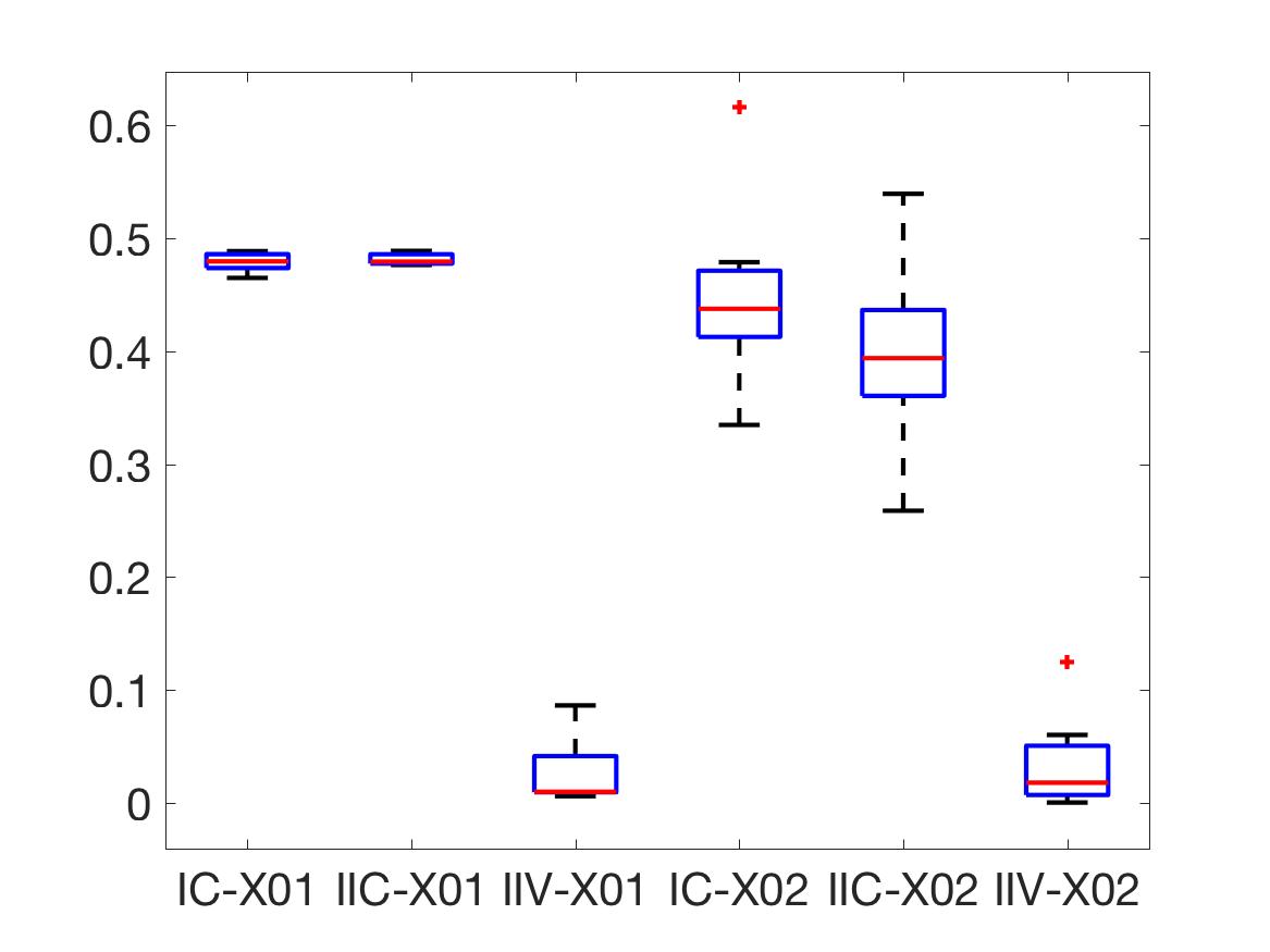
(a)

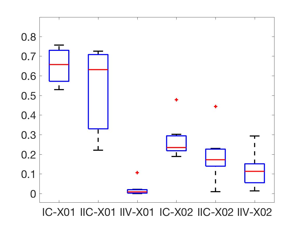
(b)

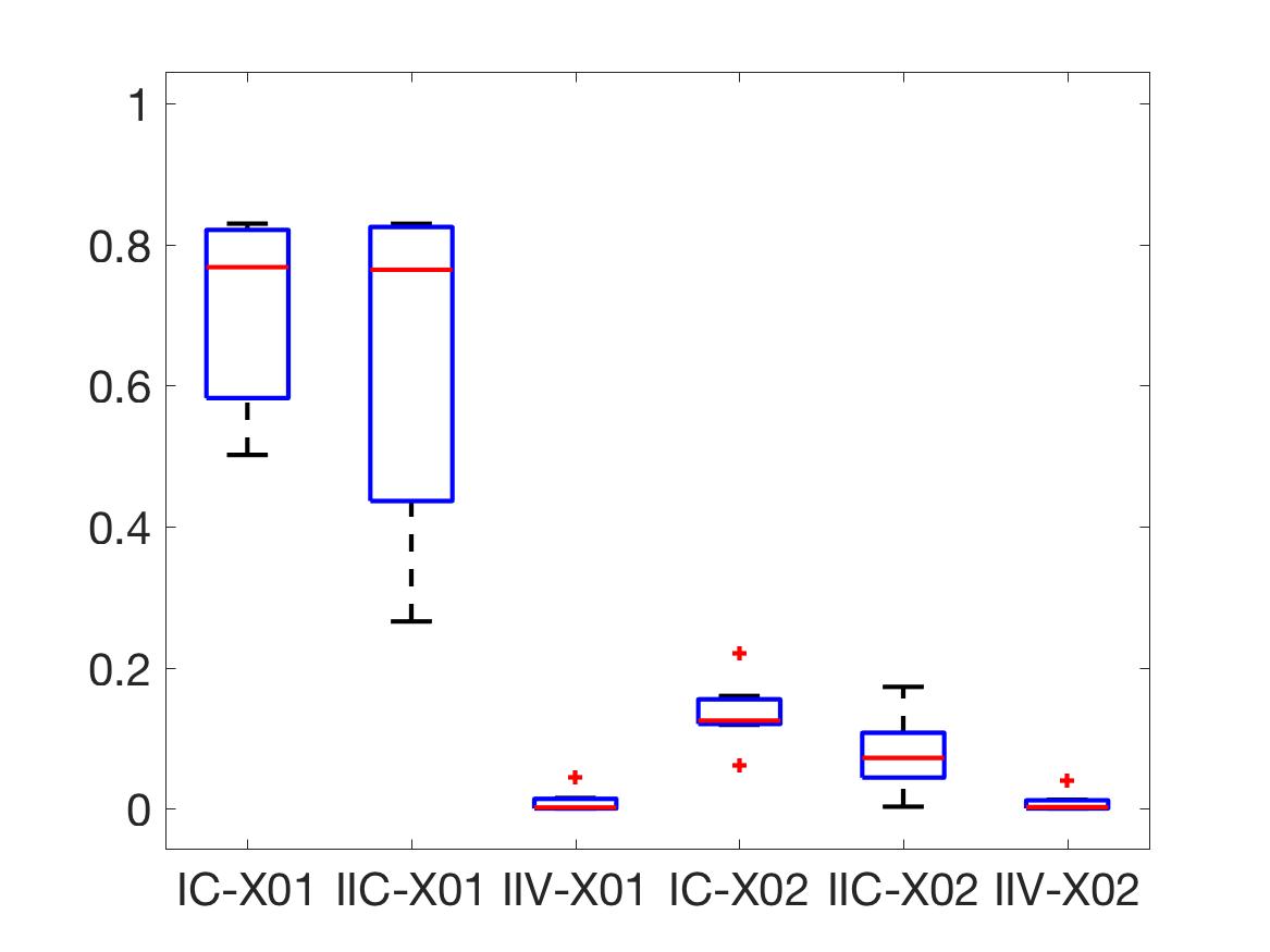
(c)

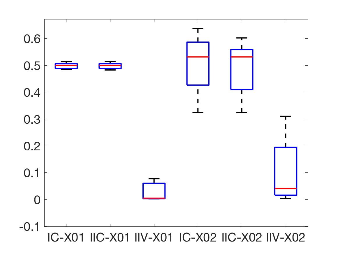
(d)

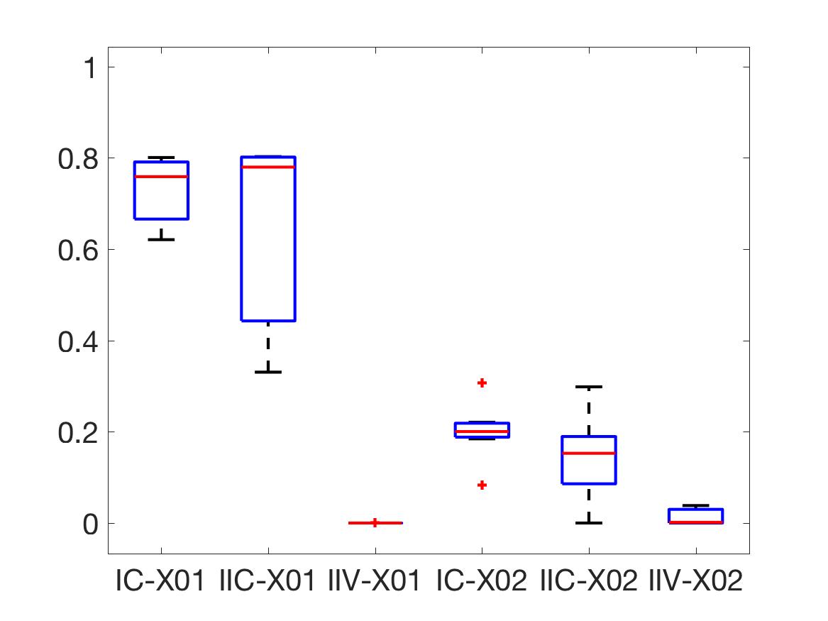
(e)

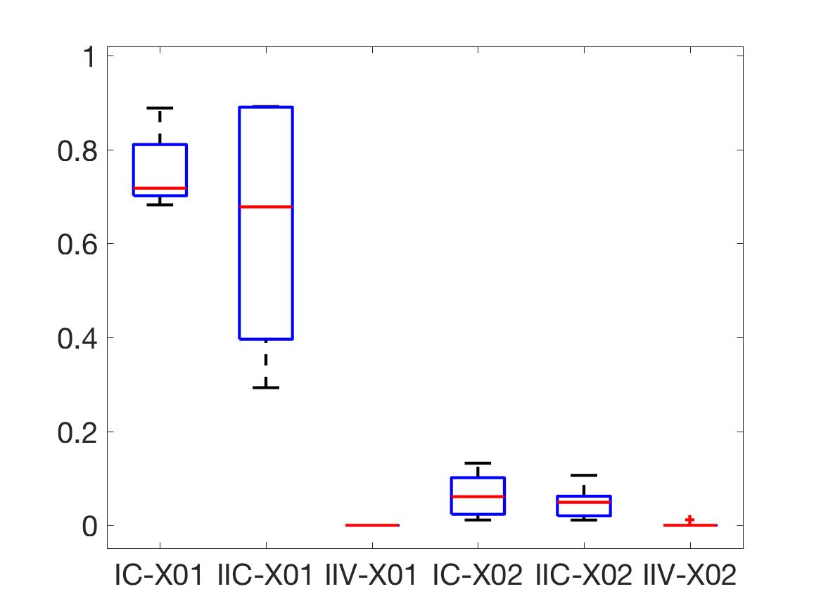
(f)

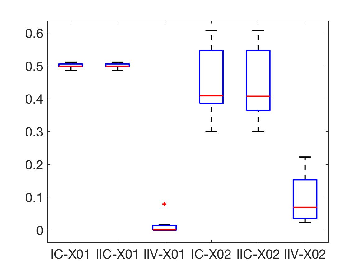
(g)

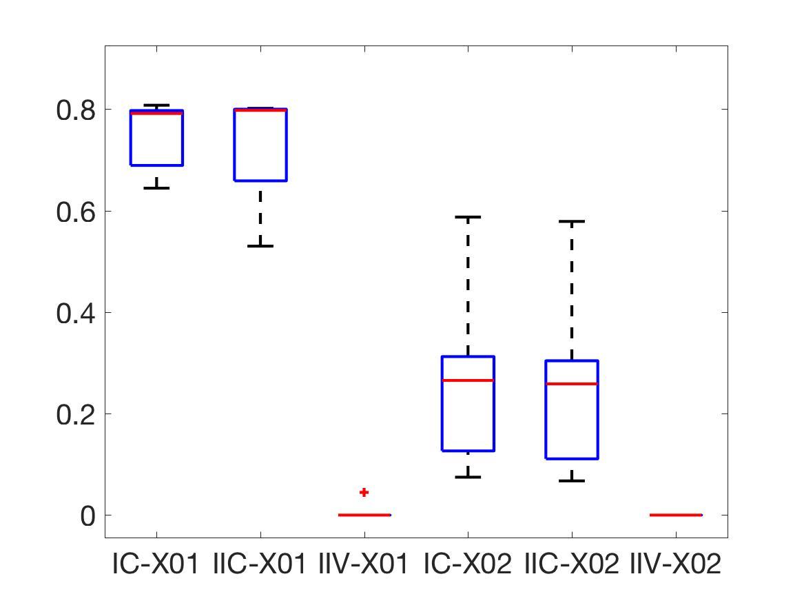
(h)

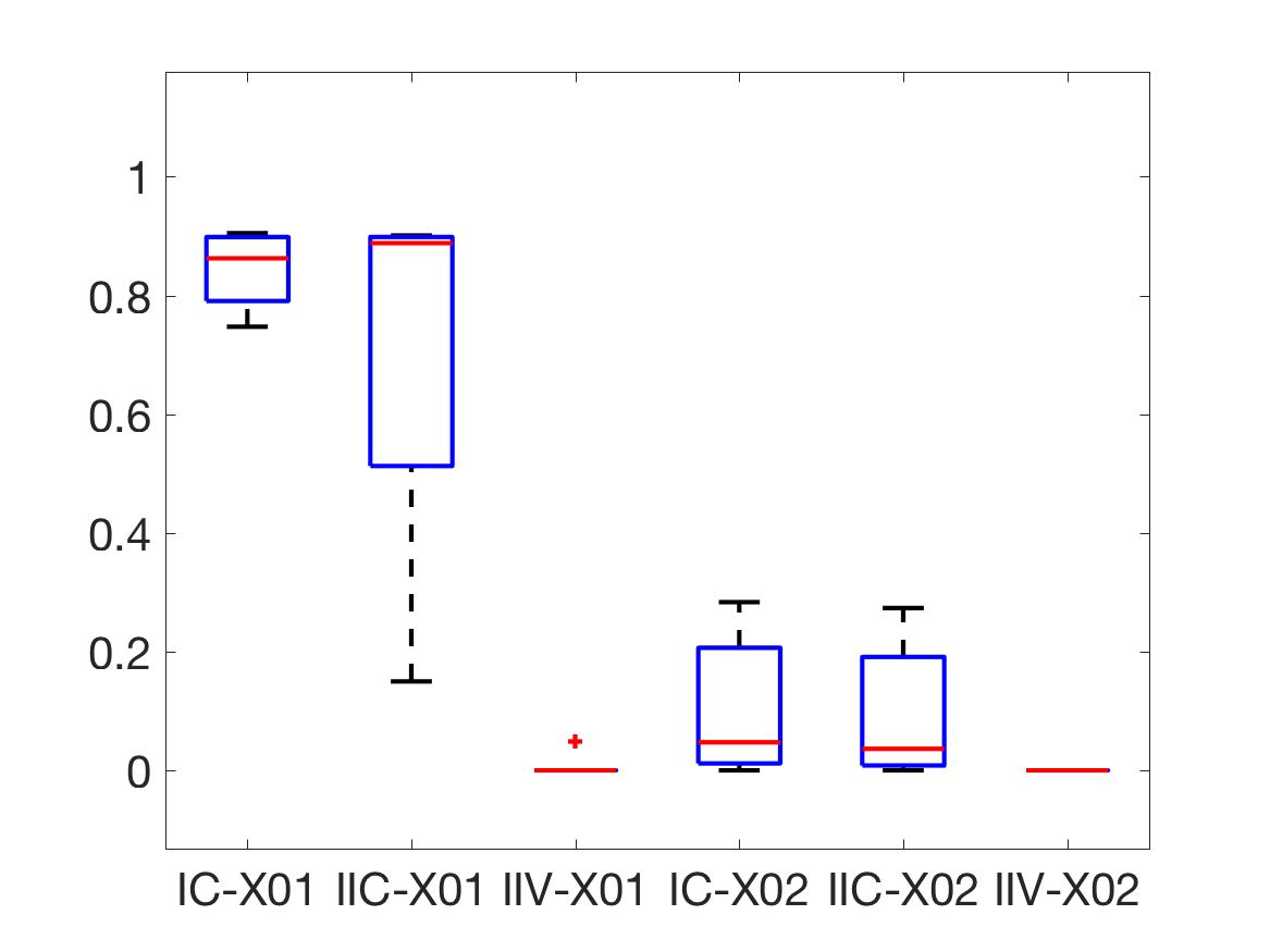
(i)

Figure 1: Results for datasets generated from forward model Model I. Columns correspond to different settings of $K$ (2, 5 and 10 respectively). Rows correspond to different settings of $M$ (10, 20 and 40 respectively). Boxplots within each subplot represent misclassification rates for 10 repeats for (from left to right), Model I with coordinate-ascent ($IC$), Model II with coordinate-ascent ($IIC$), Model II with variational Bayes ($IIV$). These are repeated twice, with random initializations ($X_{01})$, and with a greedy initialization that contains all the nonzero components from the $M$ images ($X_{02}$).

In this section, we first validate the proposed MAP-MRF framework using synthetically generated maps from two observation processes: the model specified in equations (1)-(3), as well as a simplified version without measurement noise (i.e. $Z(s)=0$). Table 1 summarizes these two models. We also compare two algorithms: a coordinate-ascent optimization algorithm and our variational Bayes algorithm. Across different settings, we compare the estimated group map to the synthetically generated ground truth group map, allowing us to assess the viability of the proposed framework as well as its robustness to modeling error.

Generative Model	Forward Model at Voxel s	Prior Model
Model I	$Y_{i}(s)=H_{i}(s)\odot X(s)+N_{i}(s)$	$H_{i},X$ $\sim$ MRF, $N_{i}(s)$ $\overset{\text{i.i.d.}}{\sim}P,P\sim$ Dir(K,1)
Model II  (proposed)	$Y_{i}(s)=H_{i}(s)\odot(X(s)+Z_{i}(s))+N_{i}(s)$	$H_{i},X$ $\sim$ MRF, $N_{i}(s)$ $\overset{\text{i.i.d.}}{\sim}P,P\sim$ Dir(K,1)

Table 1: Details of both generative models. For Model II, we have both coordinate-ascent as well as variational Bayes.

To generate the group map $X$, we simulate a $K$-level Potts model. We also generate binary masks $H_{i}$, $i=1,2,\ldots,M$, following an Ising model. For both we use random temperature parameters drawn uniformly between 0 and 1. Next, individual subject maps $Y_{i}$ are produced from $X$ and $H_{i}$, according to Model I and Model II. In section 4.1, we use datasets from Model I to evaluate our two algorithms: coordinate-ascent, as well as our proposed variational Bayes algorithm, by comparing misclassification rates. In section 4.2, we repeat this, now with synthetic datasets generated from Model II. Finally, we analyze the efficacy of our proposed MAP-MRF framework, i.e., Model II with variational Bayes, on a simulated fMRI dataset. In section 4.3, we present the estimation results, and show the robustness of the proposed MAP-MRF framework.

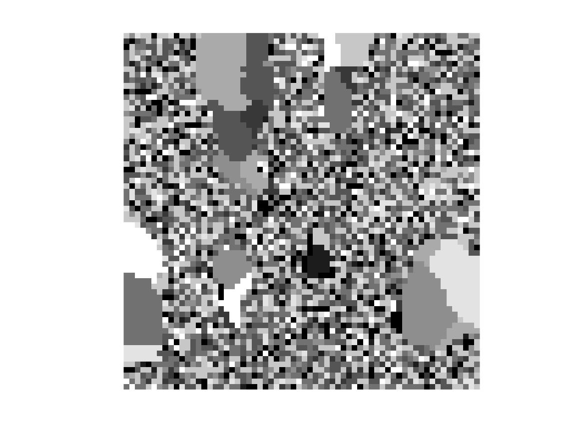
(a)

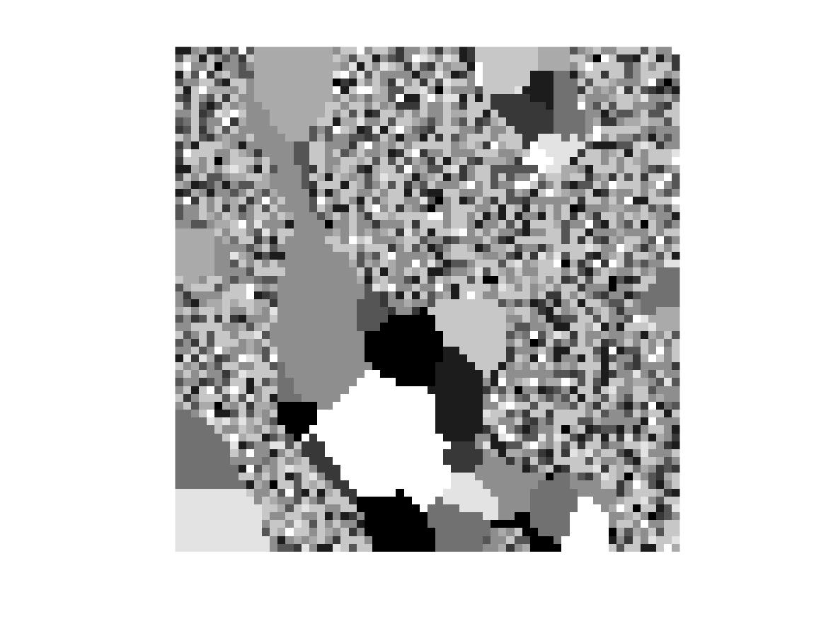
(b)

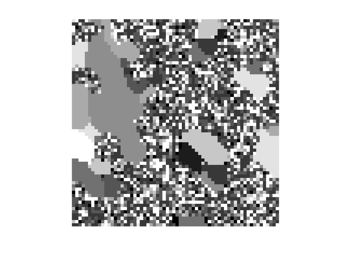
(c)

Figure 2: Figures LABEL:sub@fig:Y1-LABEL:sub@fig:Y3 show individual subject maps, $Y_{1}$, $Y_{2}$, $Y_{3}$, respectively.

(a)

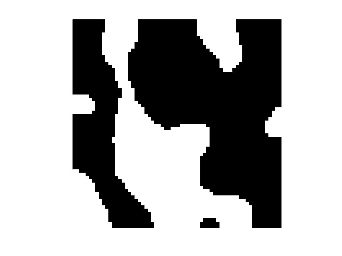
(b)

(c)

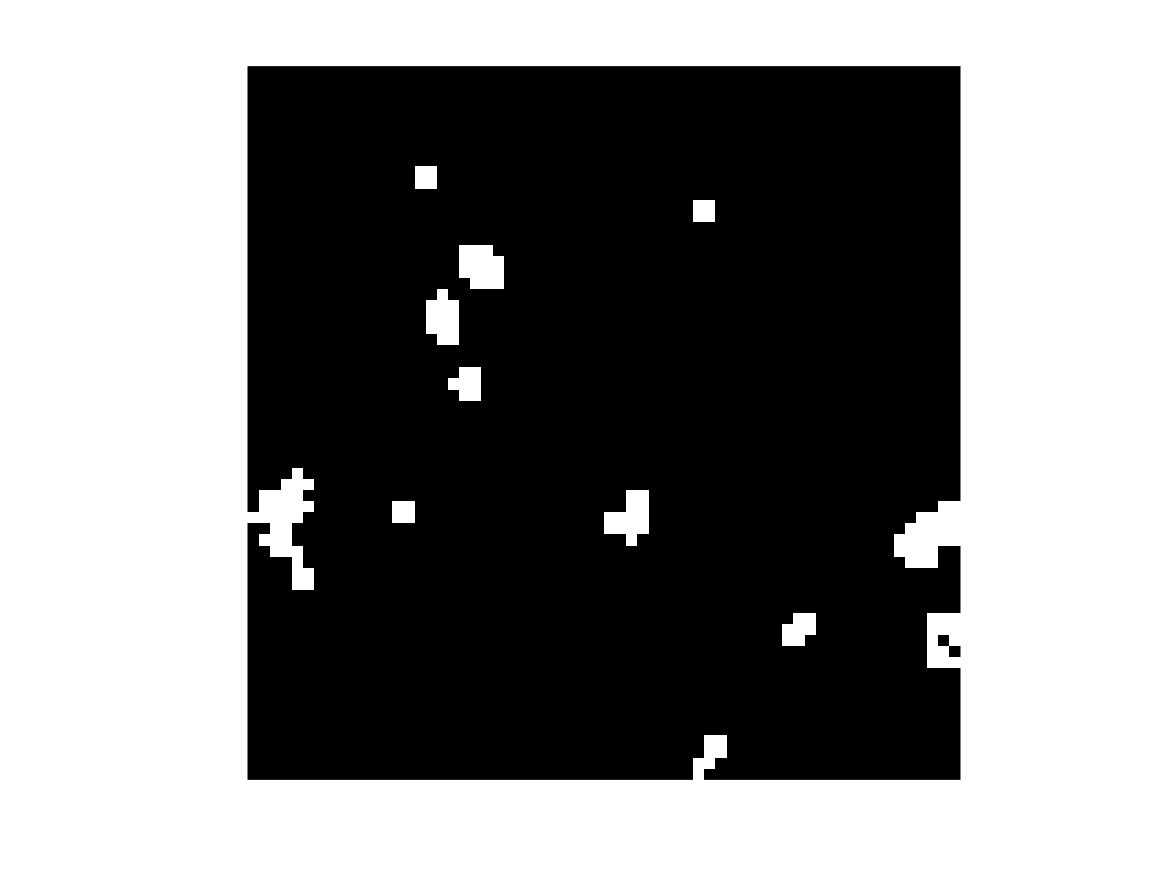
(d)

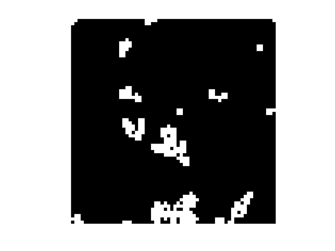
(e)

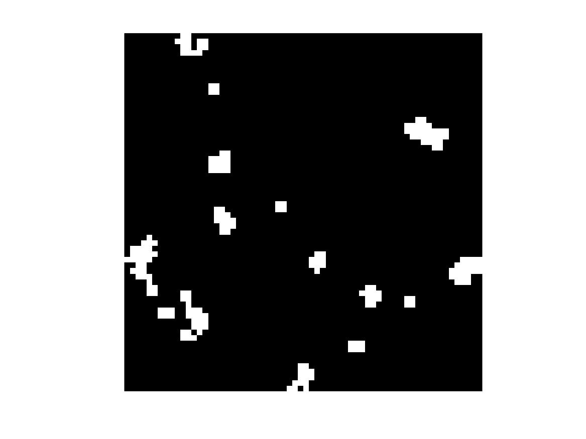
(f)

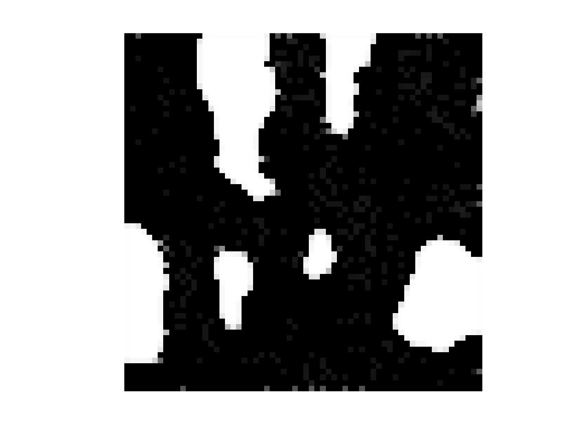
(g)

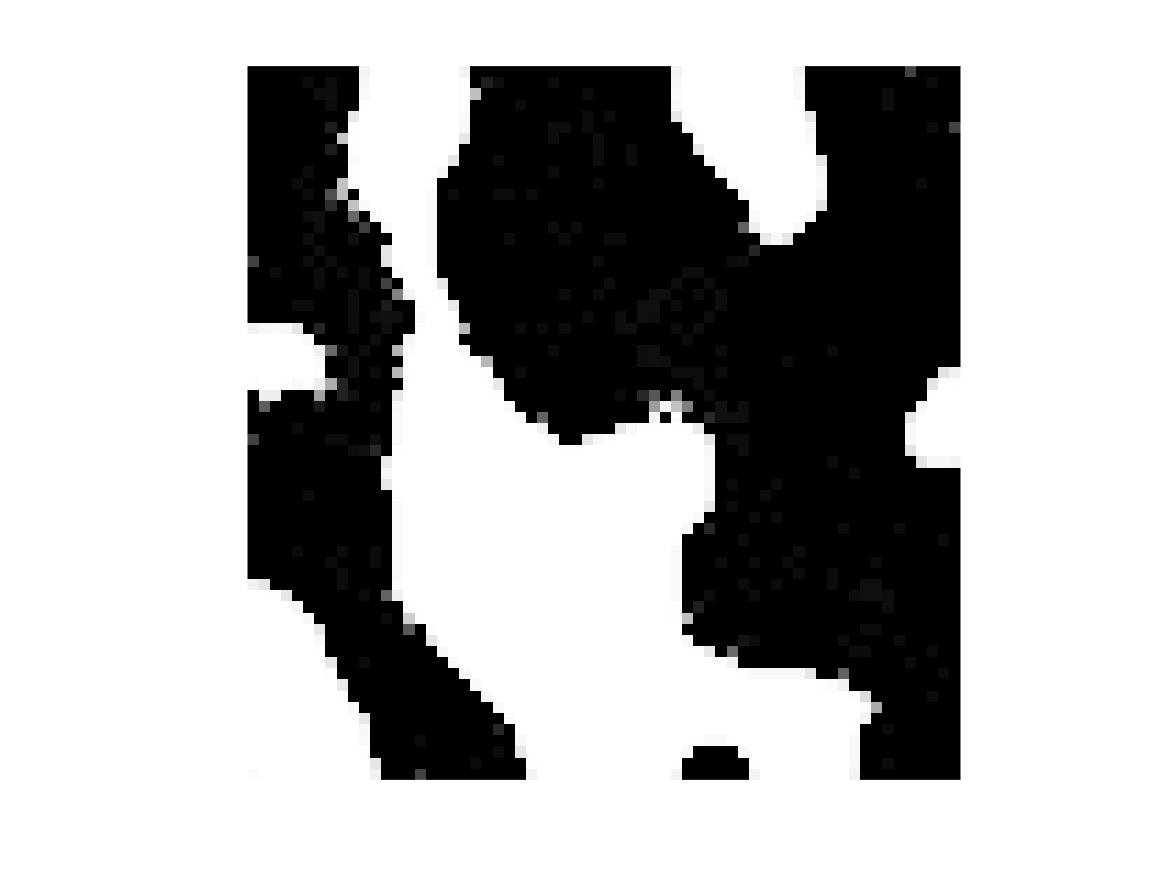
(h)

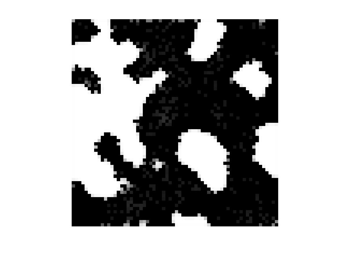
(i)

Figure 3: FiguresLABEL:sub@fig:H1_gt-LABEL:sub@fig:H3_gt show the ground truth binary masks, $H_{1}$, $H_{2}$, $H_{3}$, respectively. Figures LABEL:sub@fig:Hout1Irandom-LABEL:sub@fig:Hout3Irandom show the corresponding final estimates of the three ground truth binary masks based on Model II with coordinate-ascent and $X_{01}$ (results for Model I are similar). Figures LABEL:sub@fig:Qout1random -LABEL:sub@fig:Qout3random the final estimated probability matrices of the three ground truth binary masks based on Model I with variational Bayes and $X_{01}$.

4.1 Synthetic data from Model I

Here, we generate synthetic datasets with different numbers of labels and individuals, setting $K=2,5,10$, and $M=10,20,40$, resulting in 9 combinations. Figure 1 shows results by applying Model I (the true model), and Model II (our proposed model) to the synthetic data. Both these models are fit using coordinate-ascent. We also fit Model II using our proposed variational Bayes algorithm. In the figure, we report misclassification rates, viz. the proportion of labels in the true $X$ incorrectly labeled under the estimated $X$. We see that our model with variational Bayes outperforms other competitors, even under model-misspecification. Using variational Bayes offers a significant improvement in performance over coordinate-ascent, with almost no additional computational overhead.

To better understand the role variational Bayes plays, and the source of the improved performance, figures 3-4 present the results for the experiment with $K=10,M=40$ by implementing Model I with coordinate-ascent, Model II with coordinate-ascent and Model II with variational Bayes. In the interest of space, we show results for subjects 1, 2 and 3 (whose subject maps $Y_{1}$, $Y_{2}$ and $Y_{3}$ are shown in figure 3). Figure 3 shows the true and estimated binary masks for these three subjects for Model I, as well as Model II with variational Bayes. We see that the latter accurately recovers the truth, to which the latter bears little resemblance. Figure 4 shows how sensitivity to initialization is an important factor at play. It compares the true group-representative map $X$ to the estimated ones for the three schemes for two different initializations, random and greedy. In the latter, if a voxel is on for any of the subject maps, the corresponding voxel in the group-representative map is set to one. We see that Model II with variational Bayes is relatively insensitive to initialization, accurately recovering the true map in both cases. In this example (though not always), the other methods do well for greedy initialization but poorly for random.

(a)

Figure 4: LABEL:sub@fig:Ground_truth_group-representative_map_X the true group-representative map $X$. The leftmost column in the two rows below show two different initializations, random and greedy. The remaining columns show corresponding estimates of the group-representative map produced by (from left to right) Model I with coordinate-ascent, Model II with coordinate-ascent, and Model II with variational Bayes.

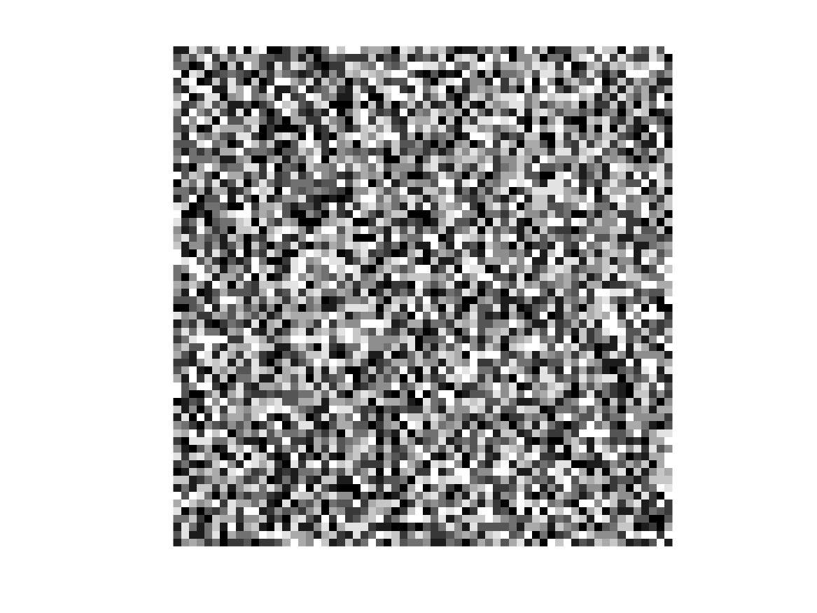
(a)

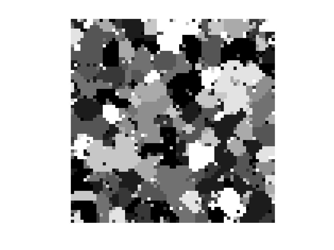
(b)

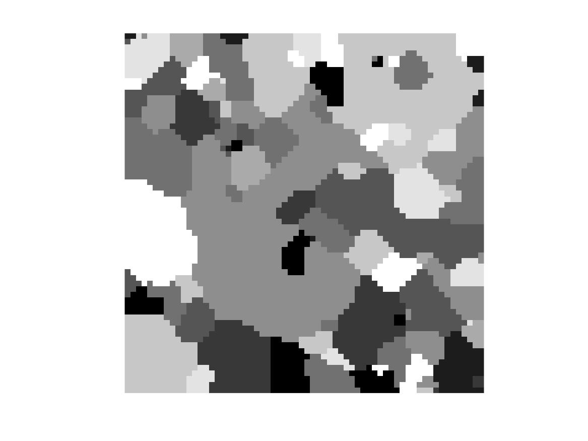
(c)

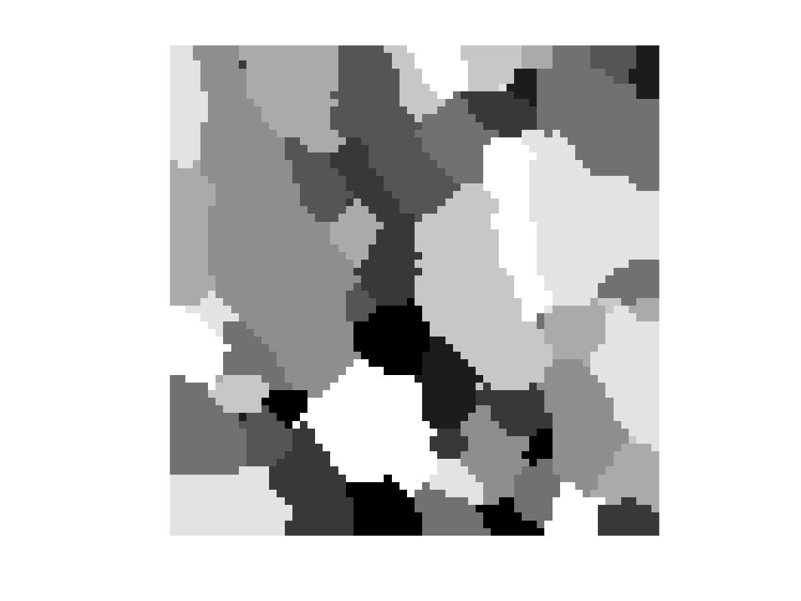
(d)

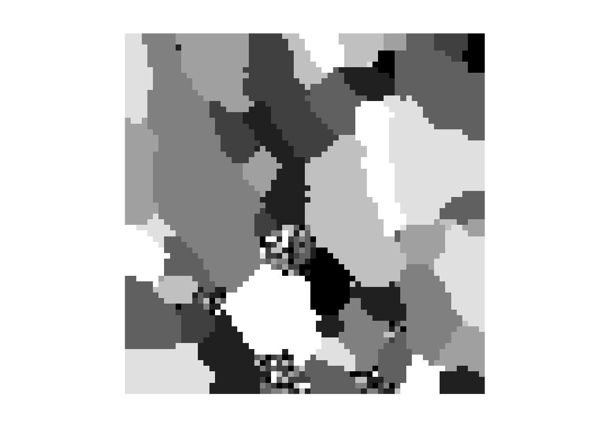
(e)

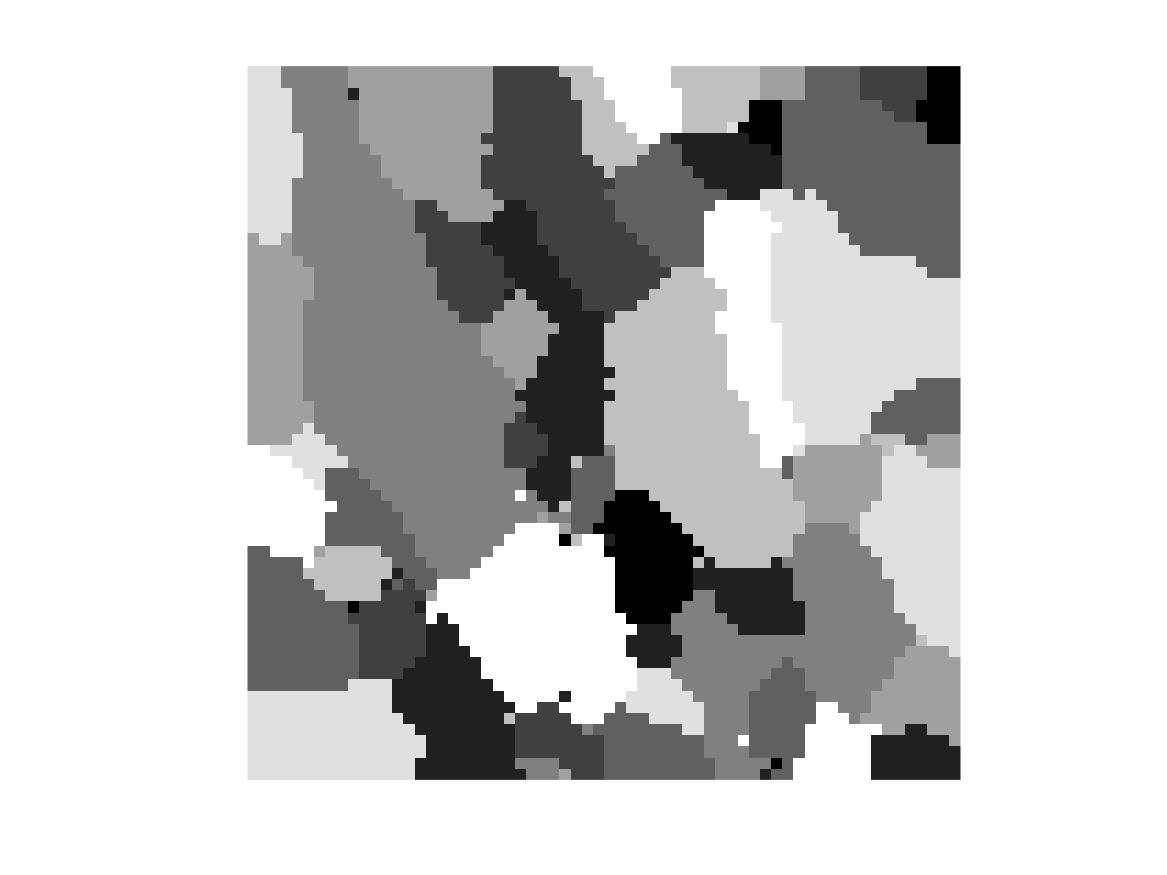
(f)

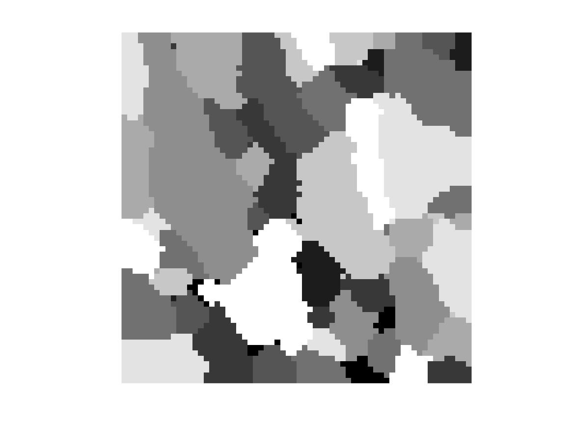
(g)

(h)

4.2 Synthetic data from Model II

In this experiment, we repeat the evaluation from the previous section, now using data with measurement noise $Z$ (see Table 1). In generating this noise, we set the noise probability $\epsilon=0.01$. Figure 5 shows a quantitative comparison of the three schemes, plotting misclassification rates of Model I with coordinate-ascent, Model II with coordinate-ascent and Model II with variational Bayes. Once again, we consider two different initializations (random and greedy) of the group-representative map $X$. This problem is harder than the earlier one, and unsurprisingly, Model I performs worst. However once again for Model II, using variational Bayes results in a markedly improved performance over coordinate-ascent, showing that even with the addition of measurement noise, coupling between $X$ and the $H_{i}$’s is sufficient to warrant a non-trivial algorithm.

In figures 7-8, we present a qualitative analysis of the effect of initialization, repeating the steps from the corresponding plots in the previous section. As before, we set $K=10$ and $M=40$. Figure 7 shows three of the images presented to the algorithms, and figures 7 and 8 show results for $H$ and $X$ respectively. Again, we see improved performance for variational Bayes in terms of its ability to avoid local optima that trap coordinate-ascent.

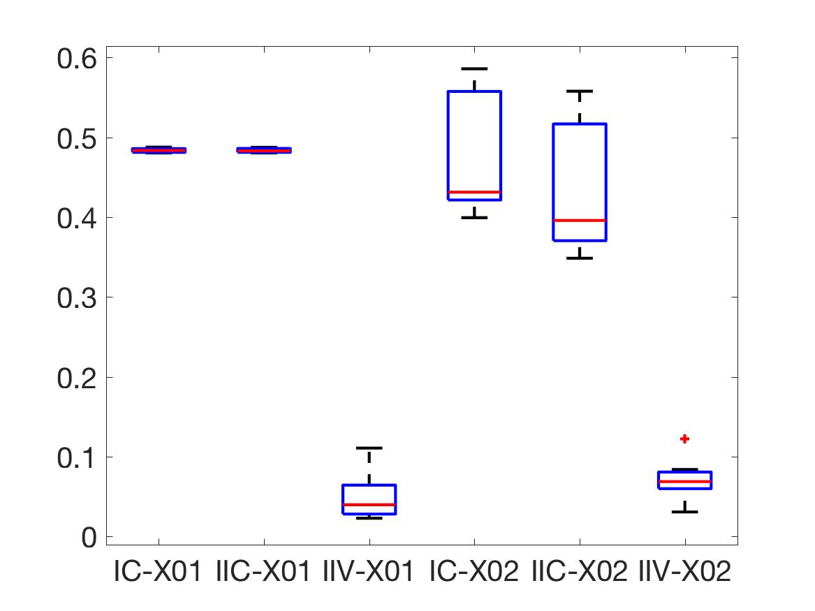
(i)

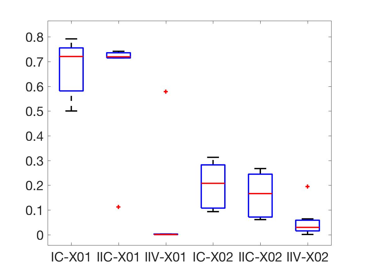
(j)

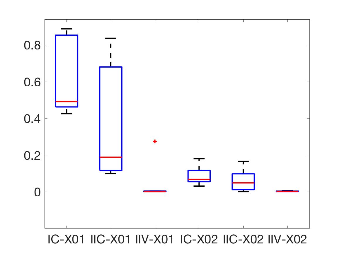
(k)

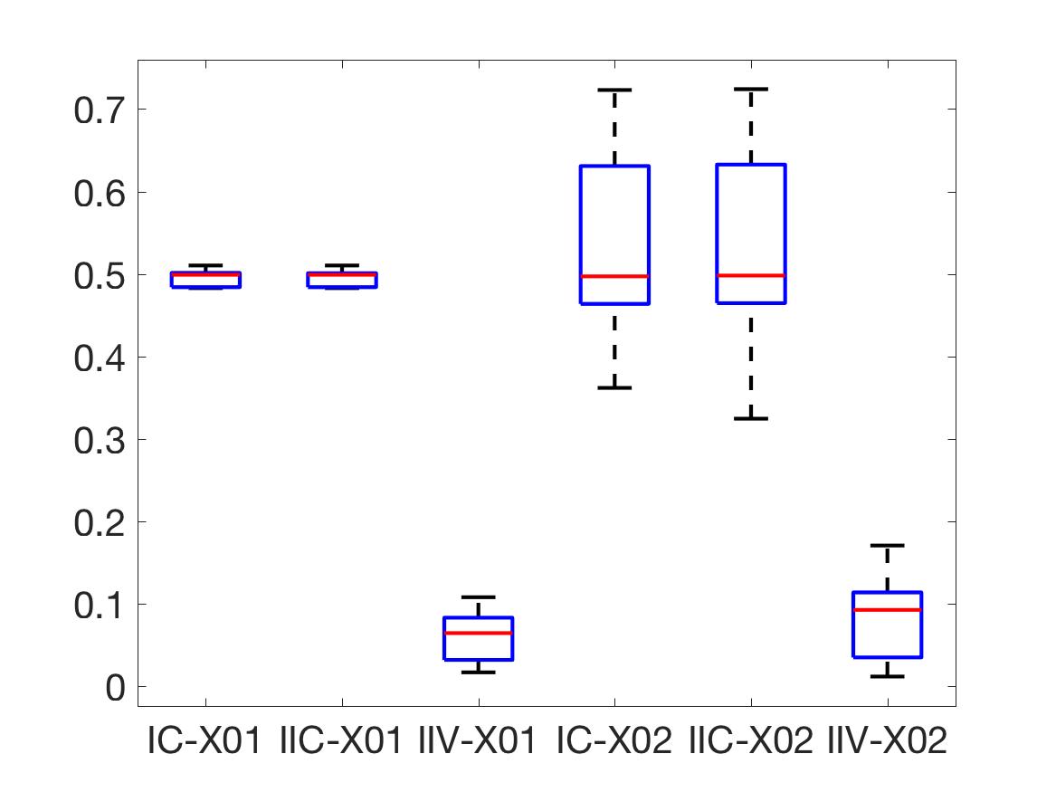
(l)

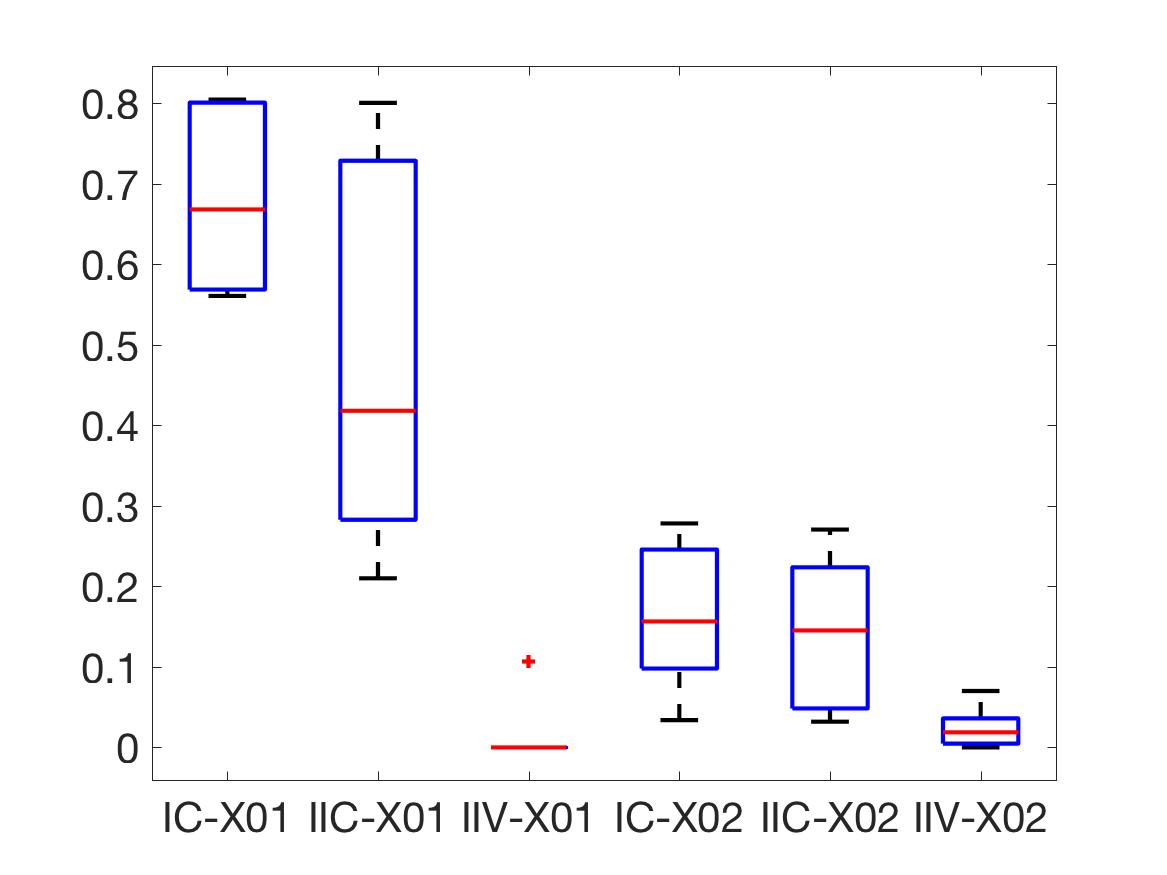
(m)

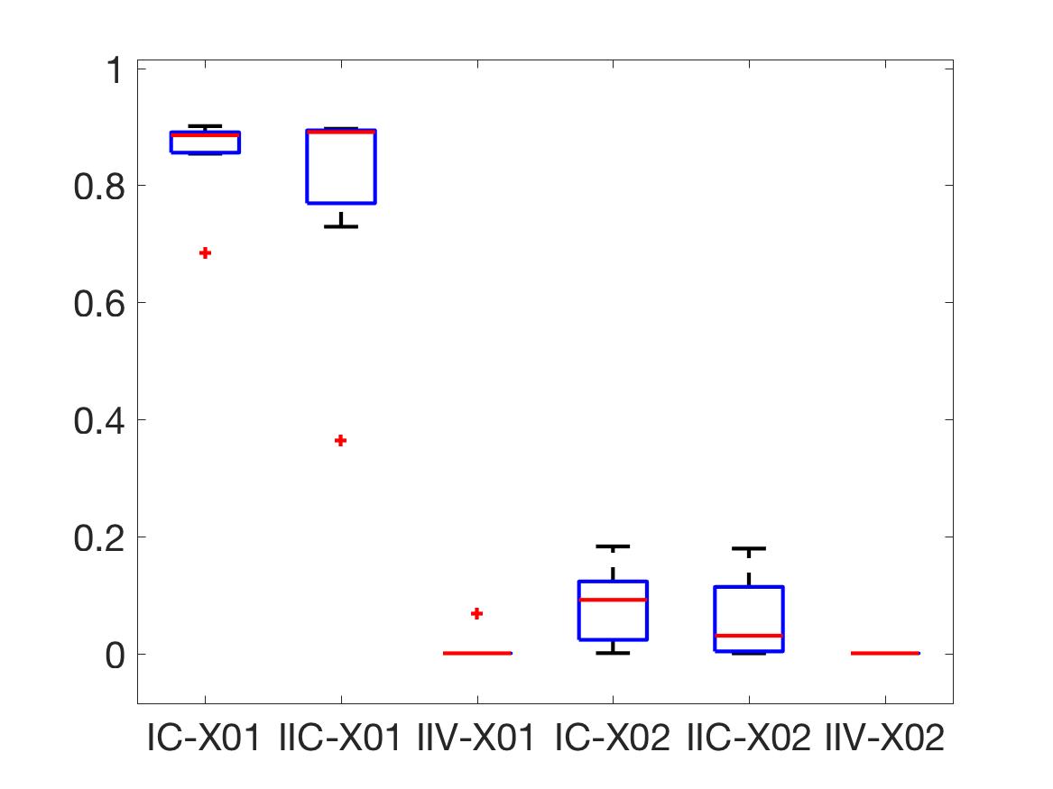
(n)

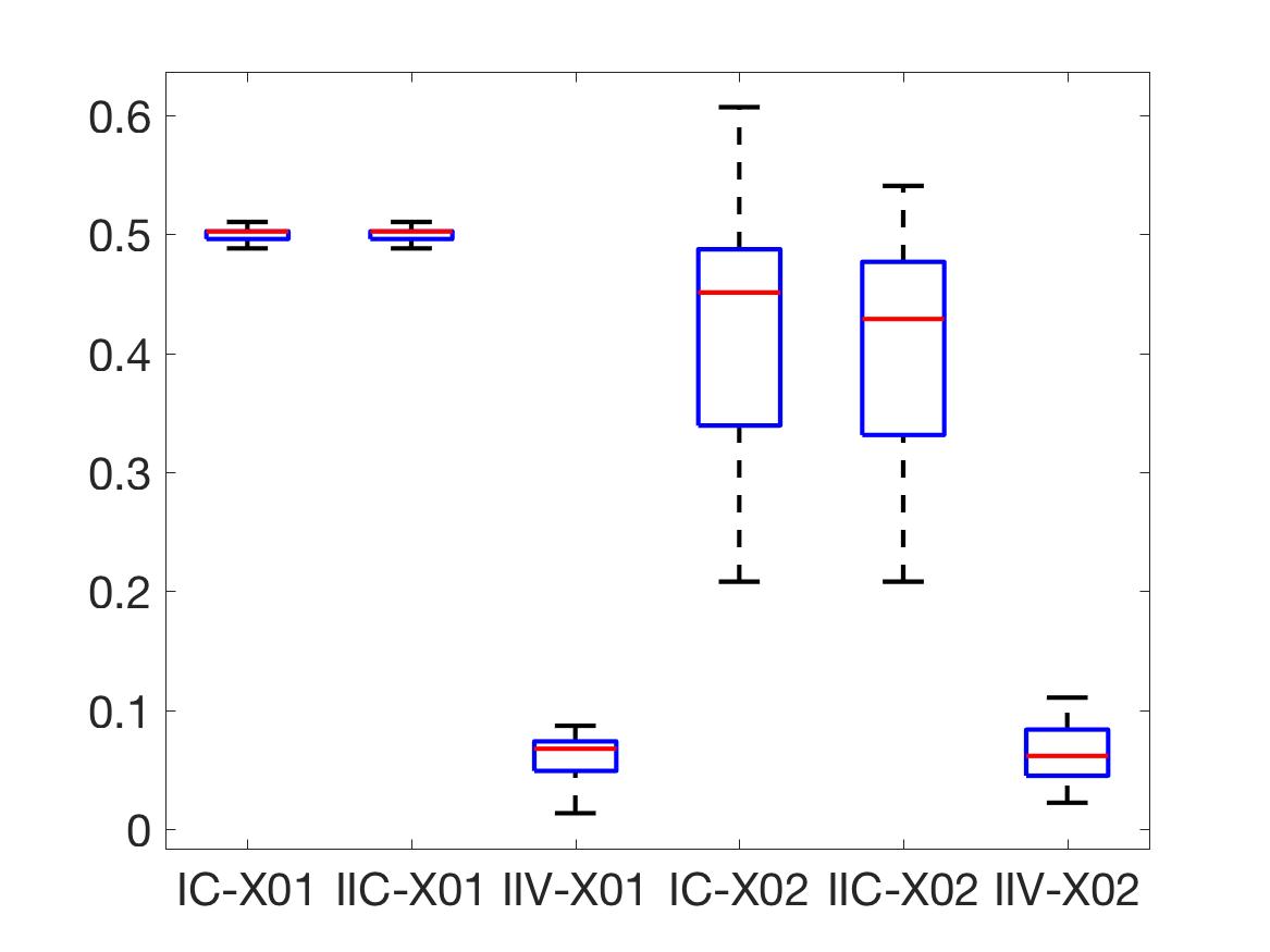
(o)

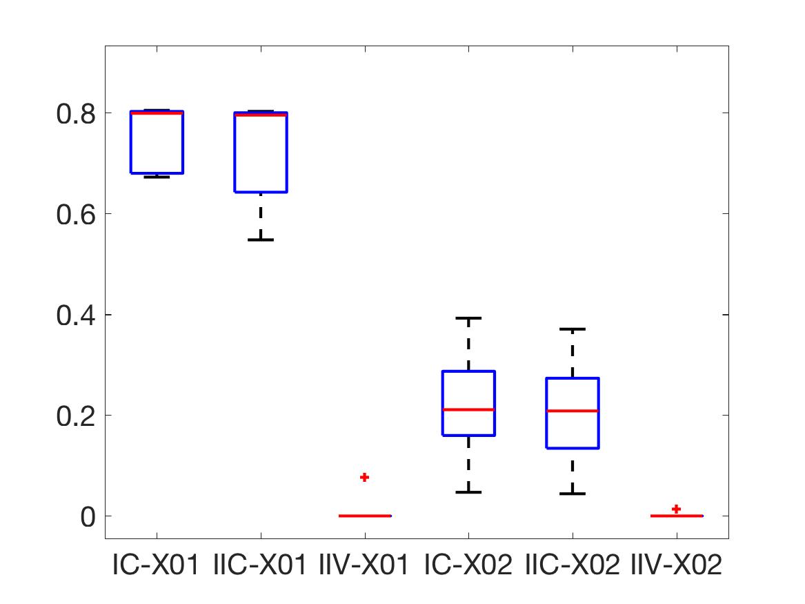
(p)

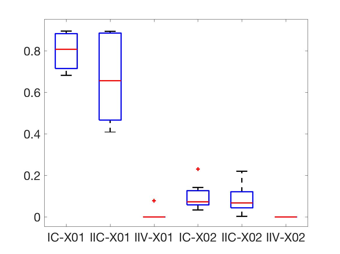
(q)

Figure 5: Results for datasets generated from forward model Model II. Columns correspond to different settings of $K$ (2, 5 and 10 respectively). Rows correspond to different settings of $M$ (10, 20 and 40 respectively). Boxplots within each subplot represent misclassification rates for 10 repeats for (from left to right): Model I with coordinate ascent ($IC$), Model II with coordinate ascent ($IIC$), Model II with variational Bayes ($IIV$). These are repeated twice, with random initializations ($X_{01})$, and with a greedy initialization that contains all the nonzero components from the $M$ images ($X_{02}$).

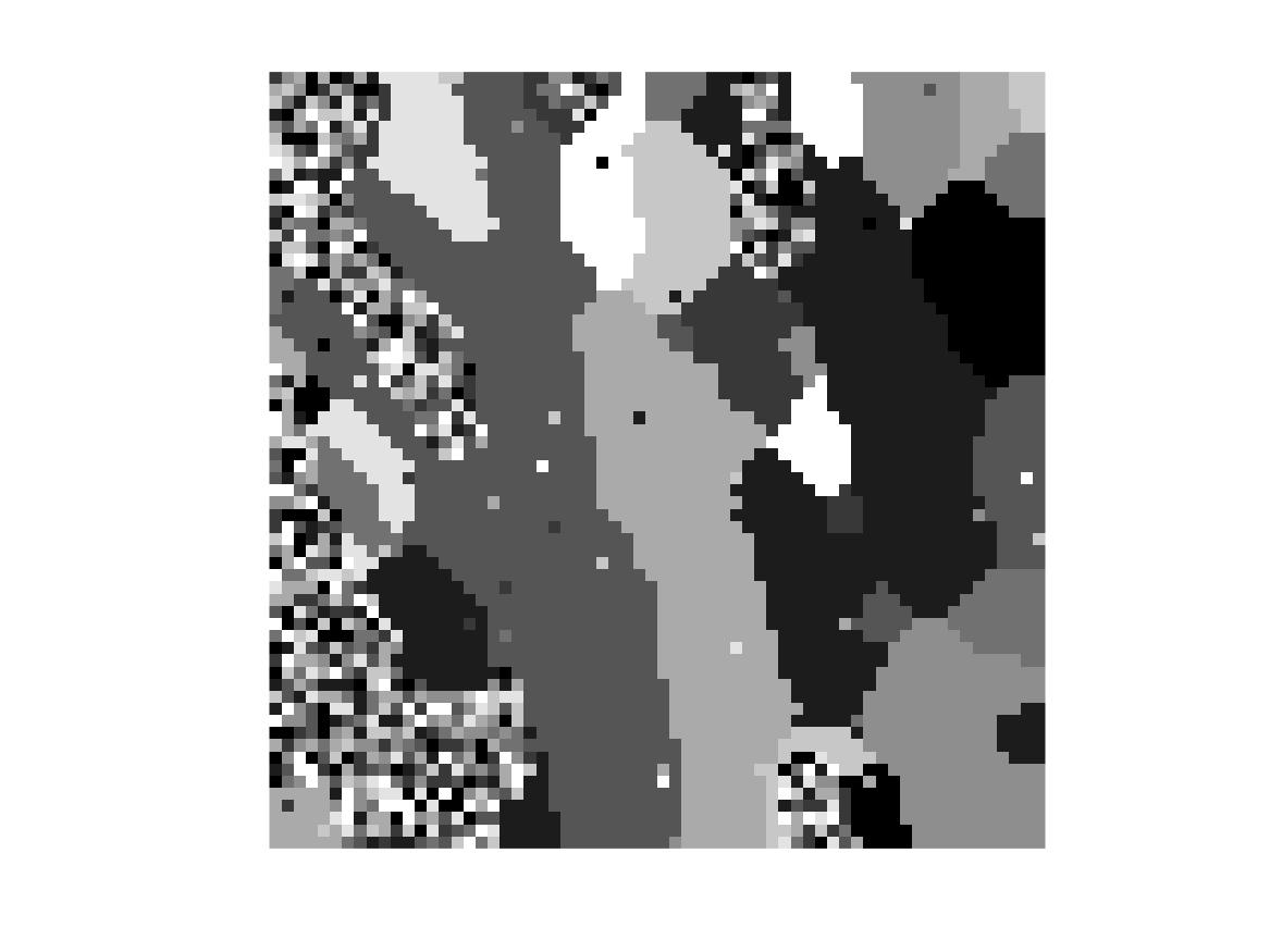
(a)

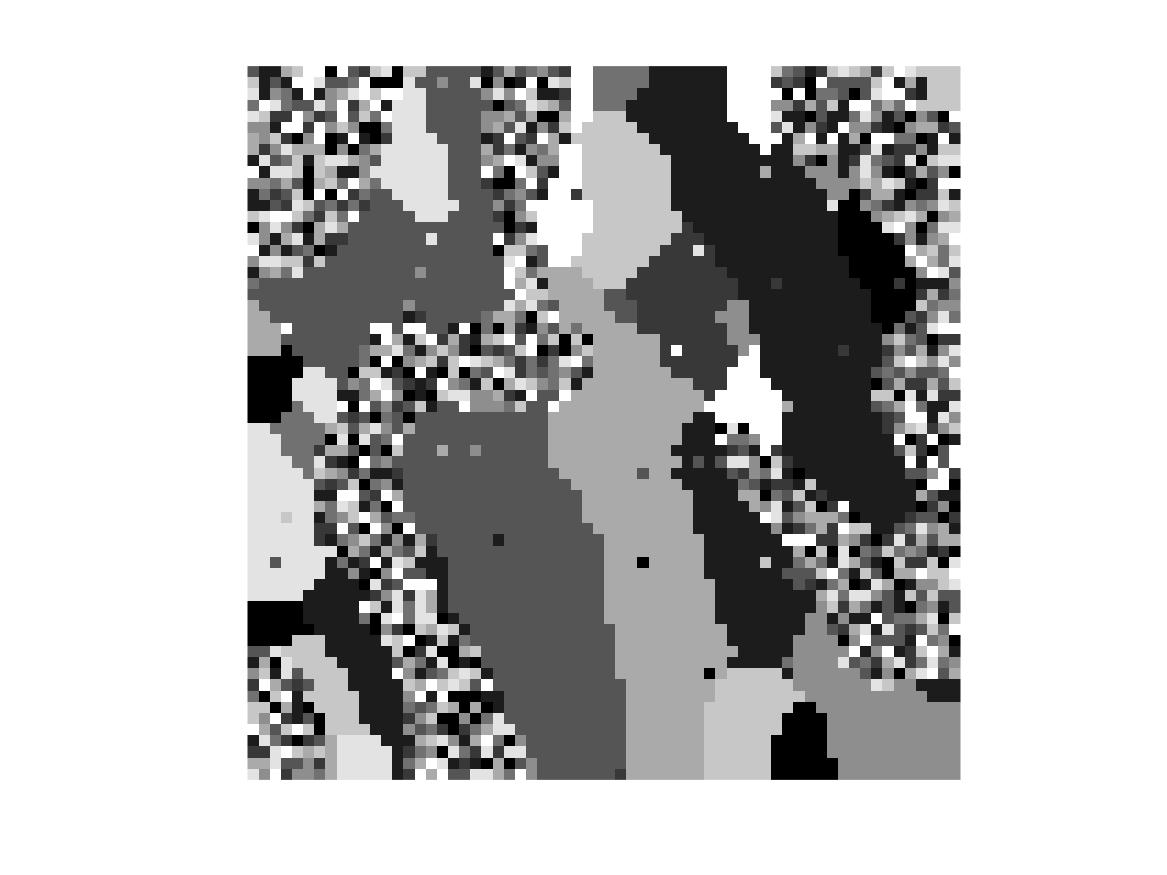
(b)

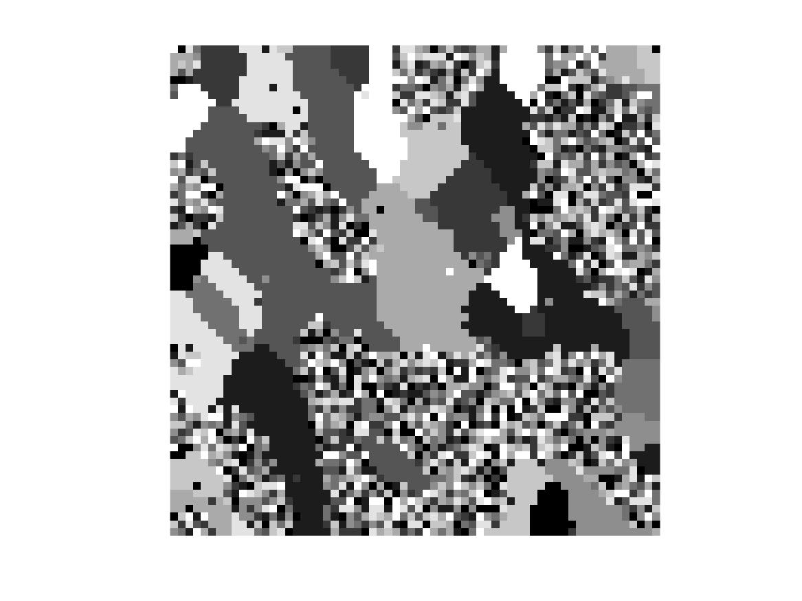
(c)

Figure 6: Figures LABEL:sub@fig:Y1 -LABEL:sub@fig:Y3: Individual subject maps, $Y_{1}$, $Y_{2}$, $Y_{3}$, respectively.

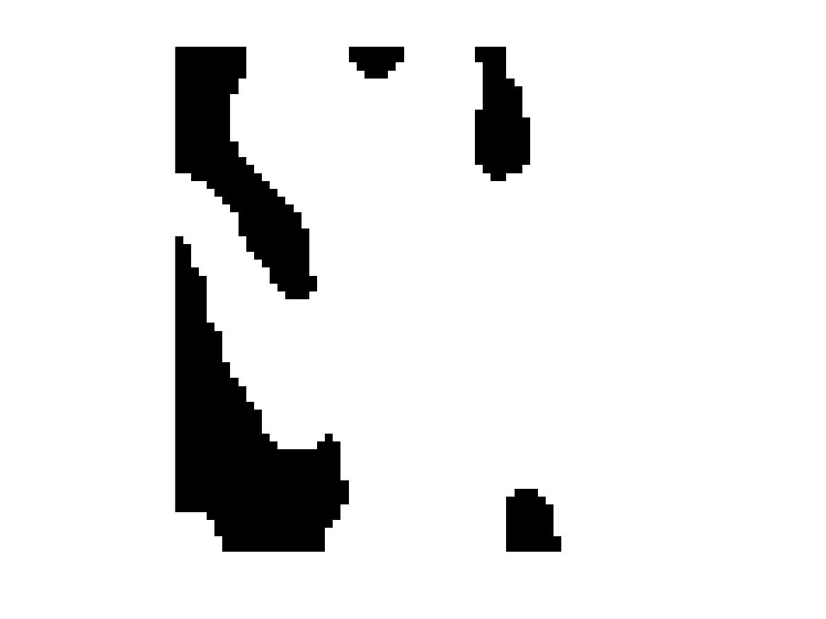
(a)

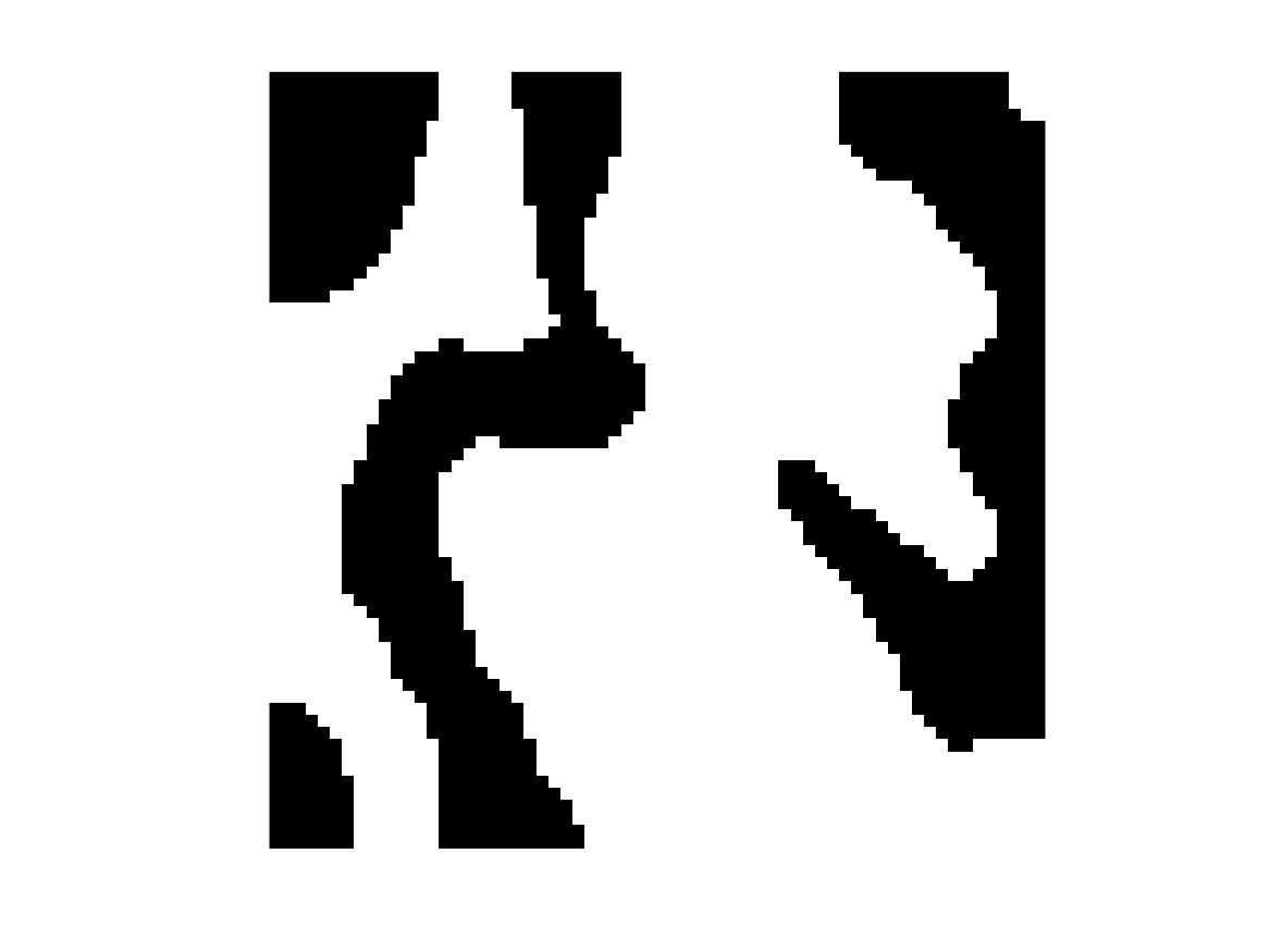
(b)

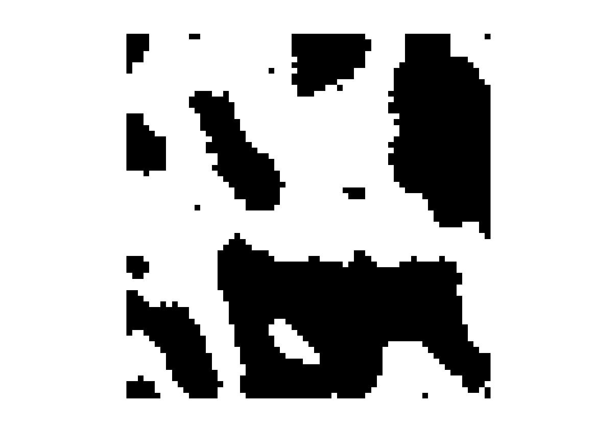
(c)

(d)

(e)

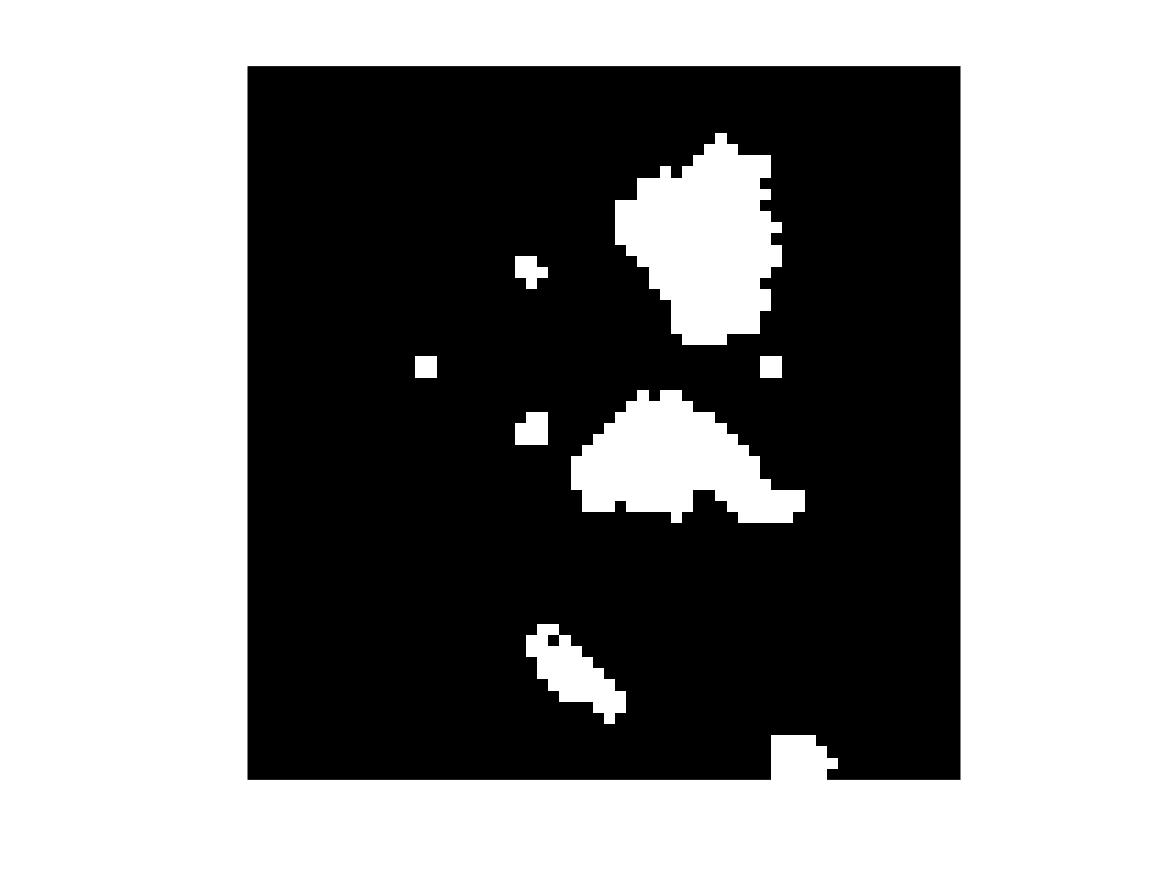
(f)

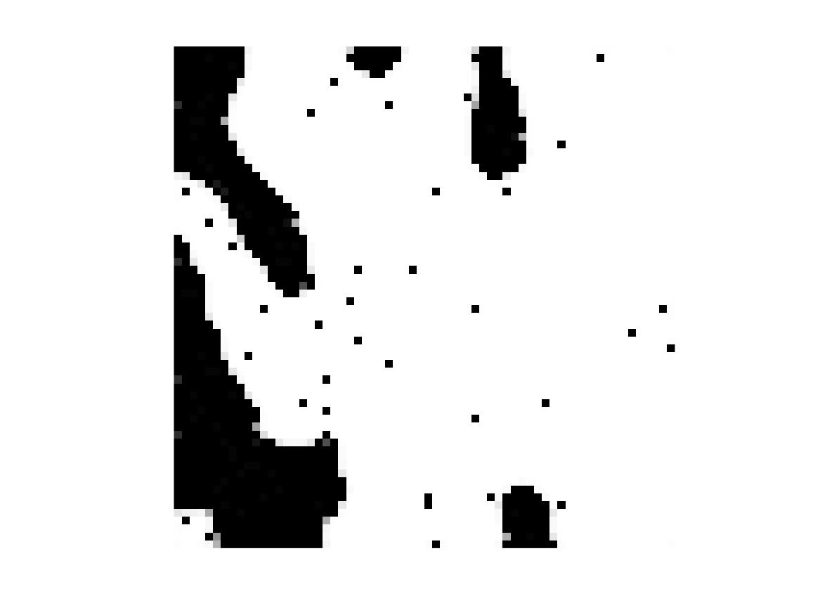
(g)

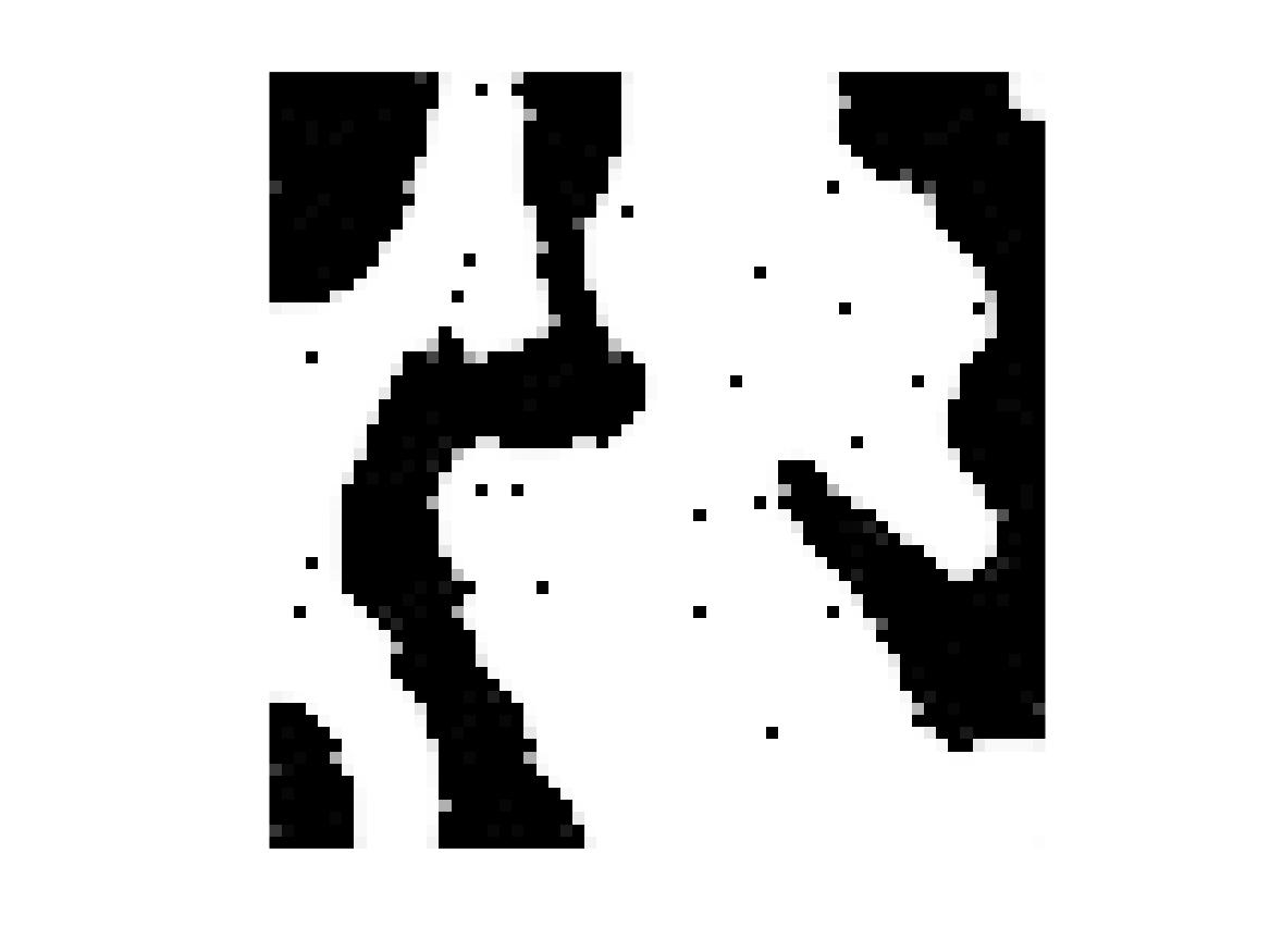
(h)

(i)

Figure 7: Figures LABEL:sub@fig:H1_gt -LABEL:sub@fig:H3_gt: the ground truth binary masks, $H_{1}$, $H_{2}$, $H_{3}$, respectively. Figures LABEL:sub@fig:Hout1IIrandom -LABEL:sub@fig:Hout3IIrandom the final estimates of the three ground truth binary masks based on Model II with coordinate ascent and $X_{01}$, $\hat{H}_{II11}$, $\hat{H}_{II21}$, $\hat{H}_{II31}$, respectively. Figures LABEL:sub@fig:Qout1random -LABEL:sub@fig:Qout3random the final estimated probability matrices of the three ground truth binary masks based on Model II with variational Bayes and $X_{01}$, $\hat{q}_{11}$, $\hat{q}_{21}$, $\hat{q}_{31}$, respectively.

(a)

Figure 8: LABEL:sub@fig:Ground_truth_group-representative_map_X the true group-representative map $X$. The leftmost column in the two rows below show two different initializations. The remaining columns show corresponding estimates of the group-representative map produced by (from left to right) Model I with coordinate ascent, Model II with coordinate ascent, and Model II with variational Bayes.

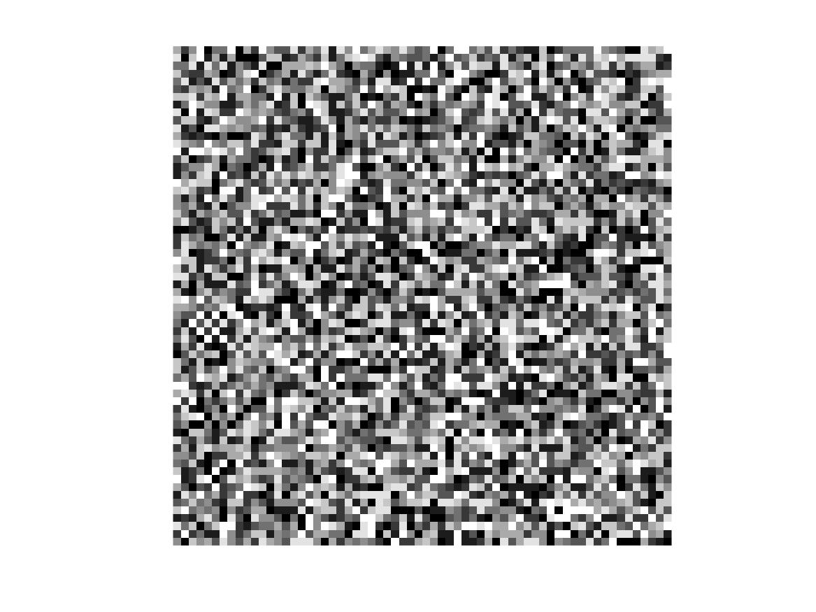
(a)

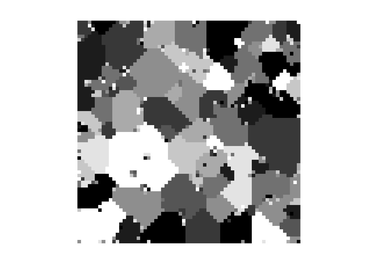
(b)

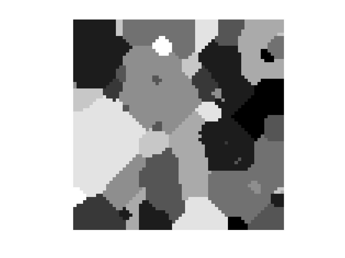
(c)

(d)

(e)

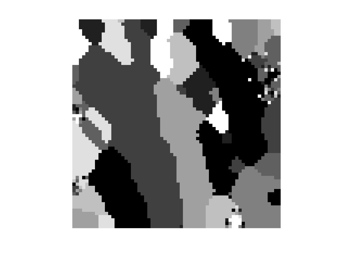
(f)

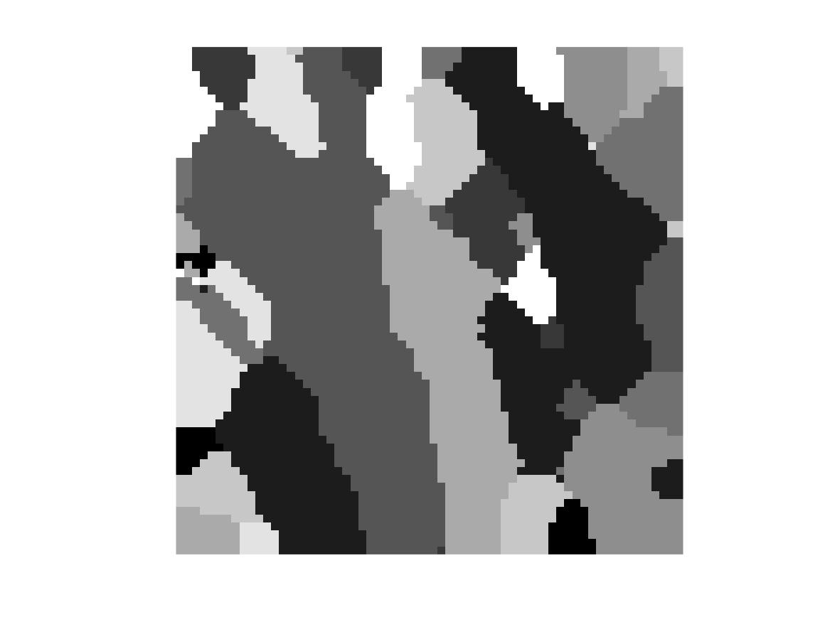
(g)

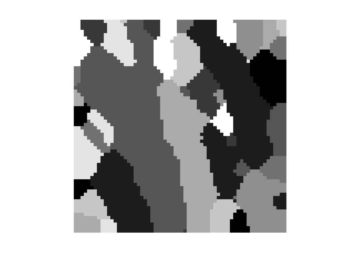
(h)

4.3 Simulated fMRI datasets

Next we test our method on simulated fMRI data generated using the SimTB toolbox for MATLAB™. SimTB facilitates the flexible generation of fMRI datasets under a model of spatio-temporal separability (Erhardt et al., 2012). Note that this generative model is not the forward model we have proposed, and to which our algorithms correspond. In keeping with the sample sizes of previous fMRI-based connectivity studies (Allen et al., 2012), we simulate $M$=30 subjects. The synthesized scans have a repetition time of $3$s/sample, with slices of size $64\times 64$ at $T$=150 time points. To maintain a reasonable computation time, we set the number of components at 30. Of these components, not all are uniformly present in all the subjects. We instead consider a subset of 17 components of interest, for each of which there is a 90% probability of occurrence in every subject. In addition, we assign to each of the remaining components, a 30% probability of occurrence. To model the spatial variability in the regions of activity under each component across the subjects, we incorporate independent normal translation, rotation, and spread. Activation centers are translated vertically and horizontally with a standard deviation of 0.3 voxels, rotated by a deviation of 1 degree, and their spatial extent (compression or expansion) is determined following the normal distribution $N(1,0.3)$. See Appendix-C for more details.

We apply the pre-processing from section 2 to this data to generate individual subject maps to input to the variational Bayes algorithm. We use this algorithm with random initialization to estimate $X_{0}$, the group-representative map. Figure 9 below plots the evolution of the estimate of $X$ over iterations of the variational Bayes algorithm until convergence, at which point, the underlying $X$ is correctly identified. In figure 10 we plot the estimated subject maps for three subjects, while figure 11 plots the evolution of the variational posterior $q_{1}(H_{1})$ of the first subject. All these estimates are clearly reasonable, indicating our modeling and computational assumptions are appropriate for fMRI images according to the standardized SimTB toolbox.

(i)

(j)

(k)

(l)

Figure 9: Estimates of the group map $X$ at iterations 1, 30, 60, 80.

(a)

(b)

(c)

Figure 10: Estimated subject maps $Y_{1}$, $Y_{2}$, and $Y_{3}$ for individuals $1,2$ and $3$.

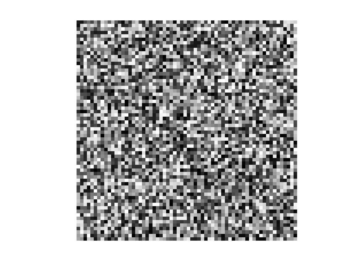
(a)

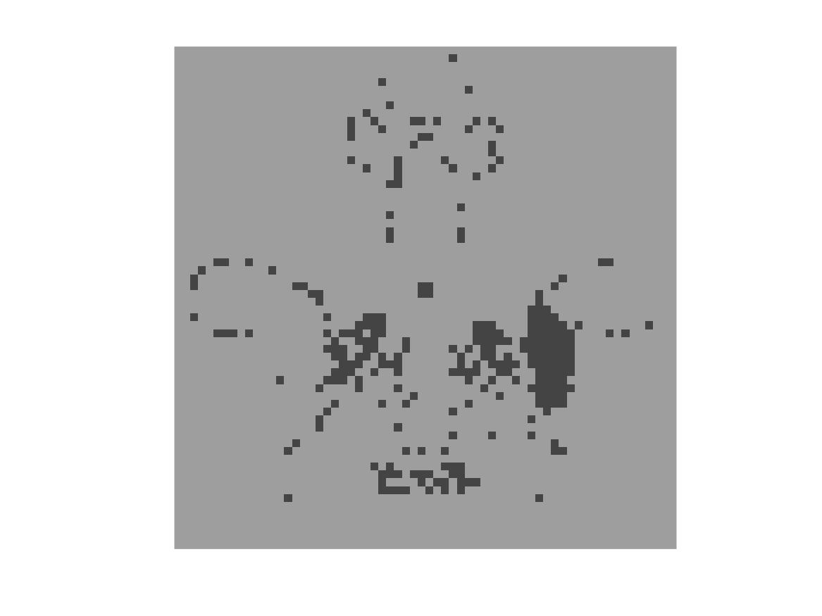
(b)

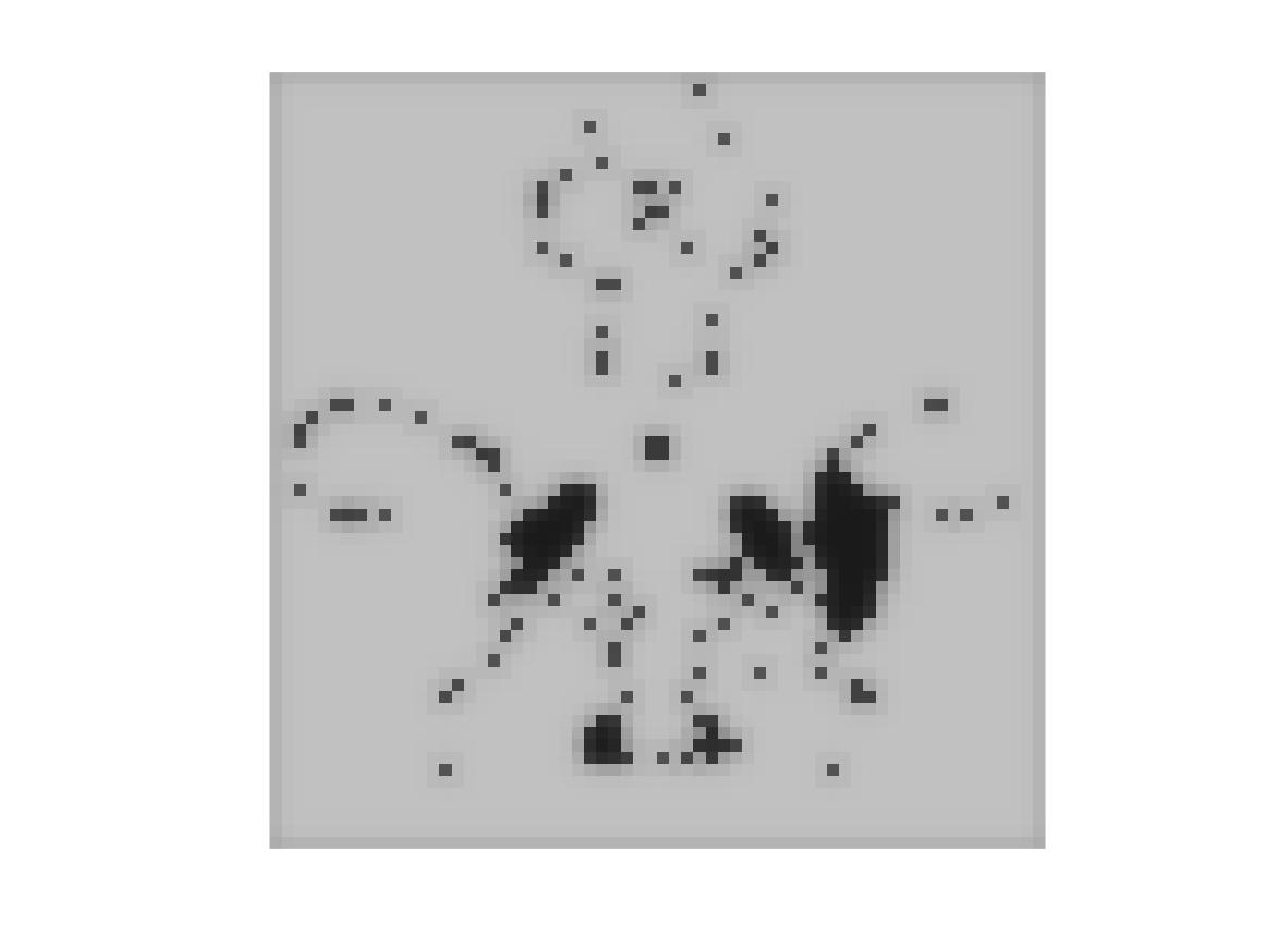
(c)

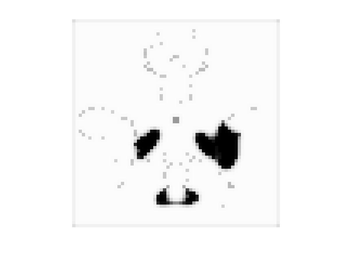
(d)

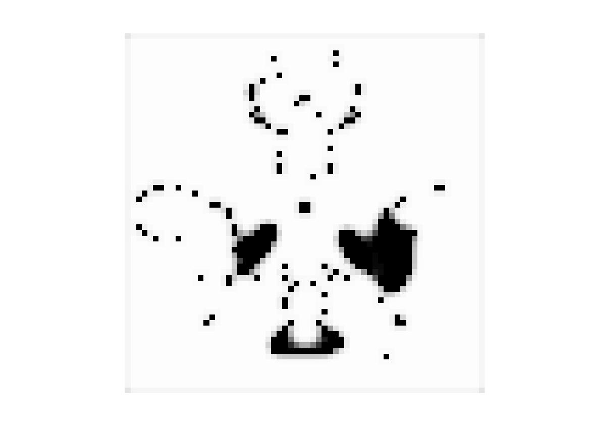
(e)

Figure 11: Estimates of the variational posterior $q_{1}$ for the mask $H_{1}$ of subject $1$ at iterations 1, 30, 60, 80, 100

Next, we use the simulated fMRI dataset to compare the robustness of the different algorithms to initialization. The leftmost column of figure 12 shows two different initializations, random (top) and greedy (bottom). From left to right, we plot the corresponding estimated group-representative maps for Model I and Model II  with coordinate-ascent, and Model II with variational Bayes respectively. Clearly, the last is the only one that a) is robust to the initialization, and b) that recovers a solution close to the ground truth. We reiterate again that this not for data generated according to any of the models.

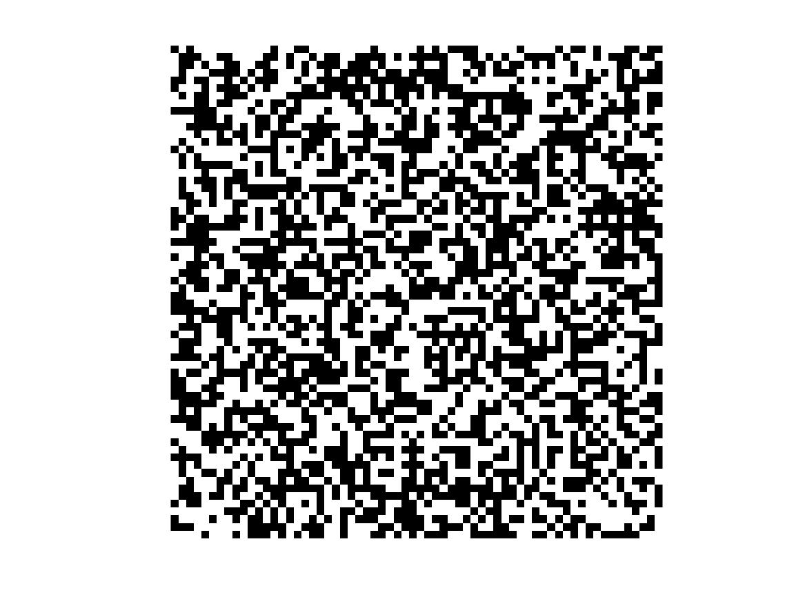
(a)

(b)

(c)

(d)

(e)

(f)

(g)

(h)

Figure 12: The leftmost column shows two different initializations (random and greedy). The remaining columns show corresponding estimates of the group-representative map produced by (from left to right) Model I with coordinate-ascent, Model II with coordinate-ascent, and Model II with variational Bayes.

5 Discussion and Conclusions

We propose a novel approach to estimate group-representative functional connectivity maps from multi-subject fMRI data. Our overall contribution is a framework consisting of two steps, a pre-processing step and a MAP-MRF model with an associated variational Bayes algorithm. Our preprocessing step overcome limitations of standard averaging and concatenation-based ICA schemes, and unlike other methods, does not require pre-registration, or the imposition of a common set of associated temporal signals. Our MAP-MRF framework involves a novel forward model that describes the generation of individual subject maps from an underlying group-representative map, as well as a novel variational . The solution to the resulting inverse problem of estimating the group-representative map is then obtained using the MAP-MRF framework.

To capture the complexity of real data, future work should explore more sophisticated prior and generative models, for instance, defining distinct inverse temperature parameters for different clique types (vertical, horizontal, diagonal). There are also opportunities for improving the generative model through modification of the noise distribution, so as to better capture the inter-subject variations.

Appendix A Data pre-processing

We represent the fMRI data of each subject $i=1,\ldots,M$ with a $T\times V$ matrix $D^{(i)}$, where $T$ is the number of time points, and $V$ the number of voxels. The $t$^th row of such a matrix contains all voxels imaged at time $t$, and the $v$^th column contains the time course of the corresponding voxel.

A.1 Outlier exclusion and dimension reduction

We first use the RV coefficient (Robert and Escoufier, 1976) to exclude individual scans showing significant disparity from the rest of the group, due to factors such as undetected scanning problems and anatomical deviations (Esposito et al., 2005). The RV coefficient for subjects $i$ and $j$ is:

$$RV(D^{(i)},D^{(j)})=Tr(Z_{i}Z_{j})/\sqrt{(Tr(Z_{i}^{2})Tr(Z_{j}^{2}))},$$ (7)

where $Tr(\cdot)$ is the matrix trace and $Z_{i}$ is the covariance matrix of subject $i$. Following Smilde et al. (2009), we calculate the $Z_{i}$’s as $Z_{i}=D_{*}^{(i)}{D_{*}^{(i)}}^{T}$, where subscript $*$ indicates zero-correction along the diagonal of $D^{(i)}$. A distance matrix is then populated using the pairwise RV coefficients and outliers are excluded from the following analysis.

Next, we reduce the number of time points in the selected data matrices $D^{(i)}$ by performing PCA. We elect to achieve maximum dimensionality reduction following a preset CPV rule of 95% for all subjects (Valle et al., 1999), and the $D^{(i)}_{T\times V}$ is reduced to $D^{(i)}_{t_{i}\times V}$ for subject $i$. The reduced data matrices are then whitened to have unit variance.

A.2 Spatial ICA

Next, we use spatial ICA to decompose the fMRI data of each subject into a set of statistically independent spatial maps and associated time courses (Calhoun et al., 2003). Assuming $P$ independent components, this decomposition is given by $D^{(i)}=A_{i}B_{i}$, where the $P\times V$ matrix $B_{i}$ denotes the spatial maps of the $P$ independent components and the $t_{i}\times P$ matrix $A_{i}$ denotes the time course of the mixing proportions.

To perform the above decomposition, we follow Calhoun et al. (2001b) and iteratively improve an initial estimate of the de-mixing matrix $W_{i}$ (the inverse of the $A_{i}$ matrix) by maximizing the independence of the source components $\hat{B}_{i}=W_{i}D^{(i)}$. For this, we utilize FastICA Toolbox 2.1 (Hyvärinen and Oja, 1998) for MATLAB™, which is chosen for its fast and robust iterative fixed-point implementation of ICA (Hyvärinen and Oja, 1997). Since the decomposition depends on the choice of the initial estimate, we run the FastICA algorithm multiple times with random initialization.

A.3 Component Clustering

The resulting components are clustered across runs using the ICASSO toolbox (Himberg and Hyvärinen, 2003), and their centrotypes are chosen as final estimates of the unknown independent components. For this clustering, we measure spatial similarity of the ICA components, as well as similarity of their corresponding time courses. For the former, we use the IMED measure (Wang et al., 2005): as shown in Nakhmani and Tannenbaum (2013), this takes into account both disagreement in the image intensity as well as pixel distance on the image lattice, and is comparatively insensitive to minor image misalignments. The IMED between two vectorized images $X$ and $Y$, normalized by their maximum intensities, is given by $R_{s}(X,Y)=(X-Y)^{T}G(X-Y)$, where $G=[g_{ij}]_{N\times N}$ is a symmetric, positive-definite weight matrix, and $g_{ij}=1/2\pi\sigma^{2}\exp\{-(i-j)^{2}/2\sigma^{2}\}$ for pixel coordinates $i=(i_{1},i_{2})$ and $j=(j_{1},j_{2})$. We normalize the IMED by dividing by the size of the image.

To measure similarity of component time courses (which can have different durations), we use the DTW distance of (Li et al., 2010), which stretches or compresses sequences locally to obtain the best possible alignment of any pair of sequences. Specifically, for two time courses $X:=[x_{1},x_{2},\ldots,x_{n}]$ and $Y:=[y_{1},y_{2},\ldots,y_{m}]$ of lengths $n$ and $m$ respectively, we define matrix $M$ to be their point-to-point Euclidean distance matrix, in which element $M_{i,j}$ is the distance $d(x_{i},y_{j})$ between $x_{i}$ and $y_{j}$. The alignment of $X$ and $Y$ may then be represented by a warping path $W=<w_{1},w_{2},\ldots,w_{K}>$, with $\max(m,n)$ ${\leq}$ $K<m+n-1$. The total cost along such a path $W$ is given by $C_{W}(X,Y)=\sum_{k=1}^{K}d_{k}$, where $d_{k}=d(x_{i},y_{j})$ and $k=1,2,\ldots,K$. The DTW distance then corresponds to the lowest-cost warping path between $X$ and $Y$, namely $R_{t}(X,Y)=\min_{W}C_{W}(X,Y)$, where $W$ is a candidate warping path.

Having calculated spatial and temporal dissimilarities between components, the overall inter-component distance for each pair of subjects is then computed as the average of the two. Components are clustered based on these distances using the Average Link method of hierarchical clustering (Murtagh, 1983). These spatial patterns are then rescaled to z-scores and thresholded using FDR-corrected p-values, to highlight the voxels that are active under each of the components.

Appendix B Additional results of Synthetic Data

These are presented in Table 2.

Dataset	M	K	Model I with coordinate ascent and $X_{01}$	Model II with coordinate ascent and $X_{01}$	Model II with variational Bayes and $X_{01}$	Model I with coordinate ascent and $X_{02}$	Model II with coordinate ascent and $X_{02}$	Model II with variational Bayes and $X_{02}$
1	10	2	0.4788	0.4813	0.0287	0.4510	0.3988	0.0348
2	10	5	0.6478	0.5261	0.0229	0.2735	0.1936	0.1174
3	10	10	0.7179	0.6556	0.0103	0.1355	0.0771	0.0092
4	20	2	0.4981	0.4979	0.0266	0.5005	0.4870	0.1090
5	20	5	0.7297	0.6298	0	0.2010	0.1445	0.0126
6	20	10	0.7550	0.6535	0	0.0653	0.0487	0.0017
7	40	2	0.5001	0.5001	0.0144	0.4537	0.4493	0.0939
8	40	5	0.7506	0.7300	0.0065	0.2698	0.2572	0
9	40	10	0.8477	0.6953	0.0071	0.0986	0.0903	0
1	10	2	0.4837	0.4837	0.0512	0.4822	0.4388	0.0717
2	10	5	0.6794	0.6389	0.0834	0.1952	0.1571	0.0522
3	10	10	0.6325	0.3466	0.0398	0.0854	0.0596	0.0018
4	20	2	0.4947	0.4947	0.0613	0.5332	0.5290	0.0829
5	20	5	0.6827	0.4747	0.0152	0.1652	0.1391	0.0236
6	20	10	0.8517	0.7936	0.0096	0.0803	0.0608	0
7	40	2	0.4997	0.4997	0.0599	0.4254	0.4022	0.0646
8	40	5	0.7493	0.7259	0.0108	0.2192	0.2034	0.0018
9	40	10	0.8023	0.6809	0.0111	0.0978	0.0856	0

Table 2: The average misclassification rates of 7 datasets generated from forward model Model I (top) and Model II (bottom). $M$ corresponds to different number of subjects and $K$ corresponds to different number of labels. $X_{01}$ is a random initialization, and $X_{02}$ is a greedy initialization that contains all the nonzero components from $Y_{1},Y_{2},\ldots,Y_{M}$, whose nonzero label at a given voxel s is the most frequent label among $Y_{1}(s),Y_{2}(s),\ldots,Y_{M}(s)$.

Appendix C Generation of the simulated fMRI dataset

We use the SimTB toolbox for MATLAB™ to generate the simulated fMRI dataset (Erhardt et al., 2012). As with (Allen et al., 2012), we simulate $M$=30 subjects in this experiment, with a repetition time $TR=3$s/sample, with slices of size $64\times 64$ at $T$=150 time points. We set the number of components at $C$ = 30. Of these components, not all are uniformly present in all the subjects. We instead consider a subset of 17 components of interest, for each of which there is a 90% probability of occurrence in every subject. In addition, we assign to each of the remaining components, a 30% probability of occurrence. To model the spatial variability in the regions of activity under each component across the subjects, we incorporate independent normal translation, rotation, and spread. Activation centers are translated vertically and horizontally with a standard deviation of 0.3 voxels, rotated by a deviation of 1 degree, and their spatial extent (compression or expansion) is determined following the normal distribution $N(1,0.3)$.

Following (Allen et al., 2012), we set the baseline component activation amplitude at 800 and draw the peak-to-peak percentage signal change from a Gaussian distribution with mean 3 and standard deviation 0.3. By default, the SimTB toolbox defines four different tissue types representing white matter, gray matter, sinus signal dropout, and cerebrospinal fluid (CSF). We set the corresponding tissue modifiers at 0.8 for white matter, 1.2 for CSF, 0.3 for the sinus signal, and 1.15 for frontal white matter, relative to the global mean intensity of 1, to approximate the statistical moments of real data, as reported in (Erhardt et al., 2012). To generate component time courses, we select the spike model for CSF, and obtain the remaining component time courses through convolution with the haemodynamic response function (HRF). Following the event-related experimental design, we set the amplitudes for component time courses to be consistent across subjects. Additionally, we simulate head motion through independent random translation and rotation, following $N(0,1)$. This distribution assumes random head motion between imaging instants, with a central position being more likely than the extremes (Erhardt et al., 2012). Finally, we add Rician noise to the generated data to simulate typical CNR levels, i.e., uniformly distributed from 0.65 to 2 (Plis et al., 2014).

To generate individual subject maps, we whiten each subject’s synthetic fMRI data matrix and reduce dimensionality, retaining 95% variance. We then examine the resulting data for irregularity using the RV coefficient, which is computed between subjects as a measure of mutual “distance”. Next, we compute the average distance of each subject’s data matrix from the rest. Those over one standard deviations away from the average distance are considered outliers and excluded from the group-estimation framework. Of the 30 subjects in our experiment, we identify eight as atypical, which are then omitted from further analysis. These subjects are observed to have high noise levels, head motion, or spatial translation of regions of activation.

Next, we decompose the synthetic data for each subject into a set of spatially independent components and associated time courses through ICA, over 20 runs with random initialization using the ICASSO toolbox (Himberg and Hyvärinen, 2003). We identify the centrotypes of the clusters of components generated over the 20 runs, which form the final estimates of the independent spatial components. We then apply average-link clustering to retain those components that are present consistently across the group of subjects. In our experiment, we observe 17 consistent components. We obtain the individual subject maps through back-projection of these consistent components. Finally, we rescale the component maps to z-scores and determine the active regions by thresholding with an FDR-corrected p-value of 0.05.

After observing that some components of the individual subjects are of the same shape but different colors, we decide to assign 1 to all previous nonzero labels as the group-representative map is characteristic of the subjects in our experiment, and summarizes their shared patterns of functional connectivity.

References

- Allen et al. (2012) Allen, E. A., Erhardt, E. B., Wei, Y., Eichele, T., Calhoun, V. D., 2012. Capturing inter-subject variability with group independent component analysis of fMRI data: A simulation study. Neuroimage 59 (4), 4141–4159.
- Ashkin and Teller (1943) Ashkin, J., Teller, E., 1943. Statistics of two-dimensional lattices with four components. Physical Review 64 (5-6), 178–184.
- Au Duong et al. (2005) Au Duong, M. V., Audoin, B., Boulanouar, K., Ibarrola, D., Malikova, I., Confort-Gouny, S., Celsis, P., Pelletier, J., Cozzone, P. J., Ranjeva, J.-P., 2005. Altered functional connectivity related to white matter changes inside the working memory network at the very early stage of MS. Journal of Cerebral Blood Flow & Metabolism 25 (10), 1245–1253.
- Baddeley and Turner (2000) Baddeley, A., Turner, R., 2000. Practical maximum pseudolikelihood for spatial point patterns. Australian and New Zealand Journal of Statistics 42, 283–322.
- Calhoun et al. (2003) Calhoun, V. D., Adali, T., Hansen, L. K., Larsen, J., Pekar, J. J., 2003. ICA of functional MRI data: An overview. In: Proc. of the International Workshop on Independent Component Analysis and Blind Signal Separation, April 2003, Nara, Japan. pp. 281–288.
- Calhoun et al. (2001a) Calhoun, V. D., Adali, T., Pearlson, G., Pekar, J. J., 2001a. A method for making group inferences from functional MRI data using independent component analysis. Human Brain Mapping 14 (3), 140–151.
- Calhoun et al. (2001b) Calhoun, V. D., Adali, T., Pearlson, G. D., Pekar, J. J., 2001b. Spatial and temporal independent component analysis of functional MRI data containing a pair of task-related waveforms. Human Brain Mapping 13 (1), 43–53.
- Cole et al. (2010) Cole, D. M., Smith, S. M., Beckmann, C. F., 2010. Advances and pitfalls in the analysis and interpretation of resting-state fMRI data. Frontiers in Systems Neuroscience 4, 8.
-
Cover and Thomas (2006)
Cover, T., Thomas, J., 2006. Elements of Information Theory. A
Wiley-Interscience publication. Wiley.
URL https://books.google.com/books?id=EuhBluW31hsC - Dempster et al. (1977) Dempster, A. P., Laird, N. M., Rubin, D. B., 1977. Maximum likelihood from incomplete data via the em algorithm. Journal of the Royal Statistical Society, Series B 39 (1), 1–38.
-
Elson and Rozanov (2012)
Elson, C., Rozanov, Y., 2012. Markov Random Fields. Springer New York.
URL https://books.google.com/books?id=wGUECAAAQBAJ - Erhardt et al. (2012) Erhardt, E. B., Allen, E. A., Wei, Y., Eichele, T., Calhoun, V. D., 2012. SimTB, A simulation toolbox for fMRI data under a model of spatiotemporal separability. Neuroimage 59 (4), 4160–4167.
- Erhardt et al. (2011) Erhardt, E. B., Rachakonda, S., Bedrick, E. J., Allen, E. A., Adali, T., Calhoun, V. D., 2011. Comparison of multi-subject ICA methods for analysis of fMRI data. Human Brain Mapping 32 (12), 2075–2095.
- Esposito et al. (2005) Esposito, F., Scarabino, T., Hyvarinen, A., Himberg, J., Formisano, E., Comani, S., Tedeschi, G., Goebel, R., Seifritz, E., Di Salle, F., 2005. Independent component analysis of fMRI group studies by self-organizing clustering. Neuroimage 25 (1), 193–205.
- Ford et al. (2003) Ford, J., Farid, H., Makedon, F., Flashman, L. A., McAllister, T. W., Megalooikonomou, V., Saykin, A. J., 2003. Patient classification of fMRI activation maps. In: Medical Image Computing and Computer-Assisted Intervention – MICCAI 2003. Vol. 2879. Springer, New York, pp. 58–65.
- Fox and Greicius (2010) Fox, M. D., Greicius, M., 2010. Clinical applications of resting state functional connectivity. Frontiers in Systems Neuroscience 4.
- Greicius et al. (2004) Greicius, M. D., Srivastava, G., Reiss, A. L., Menon, V., 2004. Default-mode network activity distinguishes Alzheimer’s disease from healthy aging: Evidence from functional MRI. Proceedings of the National Academy of Sciences of the United States of America 101 (13), 4637–4642.
- Himberg and Hyvärinen (2003) Himberg, J., Hyvärinen, A., 2003. ICASSO: Software for investigating the reliability of ICA estimates by clustering and visualization. In: Proceedings of the 13th Workshop on Neural Networks for Signal Processing, NNSP’03. pp. 259–268.
- Huettel et al. (2004) Huettel, S., Song, A. W., McCarthy, G., 2004. Functional Magnetic Resonance Imaging. 2nd Edition. Vol. 1. Sinauer Associates, Sunderland, MA.
- Hyvärinen et al. (2004) Hyvärinen, A., Karhunen, J., Oja, E., 2004. Independent Component Analysis. Vol. 46. John Wiley & Sons, Hoboken, NJ.
- Hyvärinen and Oja (1997) Hyvärinen, A., Oja, E., 1997. A fast fixed-point algorithm for independent component analysis. Neural Computation 9 (7), 1483–1492.
- Hyvärinen and Oja (1998) Hyvärinen, A., Oja, E., 1998. The FastICA MATLAB package. Http://research.ics.aalto.fi/ica/fastica/.
- Li et al. (2010) Li, Y., Chen, H., Wu, Z., 2010. Dynamic time warping distance method for similarity test of multipoint ground motion field. Mathematical Problems in Engineering (Article ID 749517), 1–12.
- Matthews (2003) Matthews, P. M., 2003. An introduction to fMRI of the brain. Wiley.
- Mckeown et al. (1998) Mckeown, M., Makeig, S., Brown, G., Jung, T.-P., Kindermann, S., Bell, A., Sejnowski, T., 1998. Analysis of fMRI data by blind separation into independent spatial components. Human Brain Mapping 6 (3), 160–188.
- Moores et al. (2015) Moores, M. T., Pettitt, A. N., Mengersen, K., 2015. Scalable Bayesian inference for the inverse temperature of a hidden Potts model. arXiv preprint arXiv:1503.08066.
- Murtagh (1983) Murtagh, F., 1983. A survey of recent advances in hierarchical clustering algorithms. The Computer Journal 26 (4), 354–359.
- Nakhmani and Tannenbaum (2013) Nakhmani, A., Tannenbaum, A., 2013. A new distance measure based on generalized image Normalized Cross-Correlation for robust video tracking and image recognition. Pattern Recognition Letters 34 (3), 315–321.
- Plis et al. (2014) Plis, S., Hjelm, D., Salakhutdinov, R., Allen, E., Bockholt, H., Long, J., Johnson, H., Paulsen, J., Turner, J., Calhoun, V., 2014. Deep learning for neuroimaging: A validation study. Frontiers in Neuroscience 8, 229.
- Robert and Escoufier (1976) Robert, P., Escoufier, Y., 1976. A unifying tool for linear multivariate statistical methods: The RV-coefficient. Journal of the Royal Statistical Society. Series C (Applied Statistics) 25 (3), 257–265.
- Schmithorst and Holland (2004) Schmithorst, V. J., Holland, S. K., 2004. Comparison of three methods for generating group statistical inferences from independent component analysis of functional magnetic resonance imaging data. Journal of Magnetic Resonance Imaging 19 (3), 365–368.
- Smilde et al. (2009) Smilde, A. K., Kiers, H. A., Bijlsma, S., Rubingh, C. M., Van Erk, M. J., 2009. Matrix correlations for high-dimensional data: the modified RV-coefficient. Bioinformatics 25 (3), 401–405.
- Valle et al. (1999) Valle, S., Li, W., Qin, S. J., 1999. Selection of the number of principal components: The variance of the reconstruction error criterion with a comparison to other methods. Industrial & Engineering Chemistry Research 38 (11), 4389–4401.
- Wainwright and Jordan (2003) Wainwright, M. J., Jordan, M. I., 2003. Graphical models, exponential families, and variational inference. Tech. Rep. 649, Department of Statistics, UC Berkeley.
- Wang et al. (2005) Wang, L., Zhang, Y., Feng, J., 2005. On the Euclidean distance of images. IEEE Trans. on Pattern Anal. and Mach. Intelligence 27 (8), 1334–1339.
- Xu et al. (2013) Xu, C.-P., Zhang, S.-W., Fang, T., Ma, M., Qian, C., Chen, H., Zhu, H.-W., Li, Y.-J., Liu, Z., 2013. Altered functional connectivity within and between brain modules in absence epilepsy: A resting-state functional magnetic resonance imaging study. BioMed Research International (Article ID 734893), 1–12.
- Xu et al. (2011) Xu, M., Chen, H., Varshney, P. K., 2011. An image fusion approach based on Markov random fields. IEEE Transactions on Geoscience and Remote Sensing 49 (12), 5116–5127.
- Yeo and Ou (2004) Yeo, B. T., Ou, W., 2004. Clustering fMRI time series, http://people.csail.mit.edu/ythomas/unpublished/6867fMRI.pdf.