Correlated Tunneling Dynamics of an Ultracold Fermi-Fermi
Mixture Confined in a Double-Well

Abstract

We unravel the correlated tunneling dynamics of a mass imbalanced few-body fermi-fermi mixture upon quenching the tilt of a double-well. The non-equilibrium dynamics of both species changes from Rabi-oscillations close to the non-interacting limit to a delayed tunneling dynamics for moderate interspecies repulsions. Considering strong interspecies interactions the lighter species experiences quantum self-trapping due to the heavier species which acts as an effective material barrier, while performing almost perfect Rabi-oscillations. The degree of entanglement, inherent in the system, is analyzed and found to be significant both at moderate and strong repulsions. To relate our findings with possible experimental realizations we simulate in-situ single-shot measurements and discuss how a sampling of such images dictates the observed dynamics. Finally, the dependence of the tunneling behavior on the mass ratio, the particle number in each species and the height of the barrier of the double-well is showcased.

I Introduction

Degenerate quantum gases in external traps offer an extraordinary level of control that enables the investigation of a multitude of many-body quantum phenomena Bloch et al. (2008). A variety of parameters can nowadays be tuned experimentally, e.g. the particle number Serwane et al. (2011); Zürn et al. (2012); Wenz et al. (2013), the interaction strength via Feshbach resonances Inouye et al. (1998); Chin et al. (2010) and the dimensionality of the confinement Greiner et al. (2002). Beyond the realization of ultracold single component bosonic Spielman et al. (2007); Fölling et al. (2007); Trotzky et al. (2008) or fermionic ensembles Zwierlein et al. (2004); Partridge et al. (2006a); Shin et al. (2006); Inguscio et al. (2007); Liao et al. (2011) also the preparation of Bose-Bose Catani et al. (2008); Thalhammer et al. (2008); Petrov (2015), Fermi-Fermi (FF) Wille et al. (2008); Köhl et al. (2005); Hadzibabic et al. (2002) or Bose-Fermi mixtures Stan et al. (2004); Ospelkaus et al. (2006); Ahufinger et al. (2005) have been achieved. Multicomponent fermionic systems consisting of different isotopes such as $\prescript{40}{}{K}$ Wu et al. (2012); Wille et al. (2008), $\prescript{6}{}{Li}$ Wille et al. (2008); Moerdijk et al. (1995), $\prescript{84}{}{Rb}$ Crane et al. (2000) or $\prescript{87}{}{Sr}$ Takamoto et al. (2006) have attracted considerable attention. They reveal intriguing features including superfluidity Chen et al. (2005); Chin et al. (2006), quantum magnetism Sowiński (2018); Hung (2011); Yannouleas et al. (2016); Koutentakis et al. (2018), insulating phases Lisandrini et al. (2017); Nataf et al. (2016); Zhou et al. (2016), phase separation processes Shin et al. (2006); Partridge et al. (2006b); Shin et al. (2008) and polaronic quasiparticles Massignan et al. (2014); Scazza et al. (2017); Schmidt et al. (2018); Mistakidis et al. .

Regarding the non-equilibrium quantum dynamics, atoms trapped in a double-well potential constitute a prototype system to study the correlated tunneling dynamics in a controllable manner. For bosons such a system represents the analog of the well-known superconducting Josephson junction Albiez et al. (2005); Zöllner et al. (2008a); Dounas-Frazer et al. (2007); Salgueiro et al. (2007). The bosonic Josephson junction exhibits various experimentally observed Albiez et al. (2005) intriguing phenomena, such as Josephson oscillations, $\pi$ modes, macroscopic quantum self-trapping Bloch (2005); Smerzi et al. (1997); Raghavan et al. (1999); Milburn et al. (1997); Sakmann et al. (2014, 2010); Sakmann (2011) and correlated pair tunneling Chatterjee et al. (2010); Zöllner et al. (2008b, a, 2006a, 2006b); Ishmukhamedov and Ishmukhamedov (2018). An extension is provided by multicomponent bosonic setups trapped in a double-well evincing for instance coherent quantum tunneling and self-trapping Kuang and Ouyang (2000), collapse and revival of population dynamics Sun and Pindzola (2009); Naddeo and Citro (2010), symmetry breaking and restoring scenarios Satija et al. (2009) and counterflow superfluidity Hu et al. (2011). Turning to the fermionic tunneling properties, the spin-polarized fermionic gas in a double-well has also been intensively studied mainly in three-dimensions unveiling coherent Josephson dynamics of two superfluid samples Valtolina et al. (2015); Spuntarelli et al. (2007), temperature dependent deformations of the density profile Salasnich et al. (2010) and incoherent single-particle oscillations Macri and Trombettoni (2013). However, the tunneling dynamics of multicomponent fermionic systems has received much less attention Sowiński et al. (2016); Tylutki et al. (2017); Harshman (2017); Paraoanu et al. (2002); Burchianti et al. (2018). This includes the investigation of the dynamical properties of few atom FF mixtures confined in a double-well potential in relation to the few-body eigenspectrum Sowiński et al. (2016), the necessity of the renormalization of the tunneling frequency in few Fermi polaron systems Tylutki et al. (2017) and the observation of Josephson oscillations in three-dimensional setups Paraoanu et al. (2002); Burchianti et al. (2018). Besides the above-mentioned studies a systematic study of the FF mixture tunneling dynamics in a one-dimensional double-well covering the weak to strong interspecies correlation regimes has not been reported. In this setup, it would be particularly interesting to examine how the interspecies correlations modify the tunneling properties of the mixture i.e. the Josephson-like oscillations, quantum self-trapping or a more complex motion. Since the fermions of each species are spin-polarized the question of induced intraspecies correlations occurs. Another intriguing prospect is to analyze the interplay between the two fermionic clouds during the evolution and to examine whether one species can act as an effective material barrier for the other one, a result that is already known for bosons Pflanzer et al. (2009, 2010). To track the non-equilibrium dynamics of the FF mixture we utilize the Multi-Layer Multi-Configurational Time-Dependent Hartree Method for Atomic Mixtures (ML-MCTDHX) Krönke et al. (2013), being a variational method that enables us to capture all the important particle correlations.

Motivated by the recent few fermion experiments Serwane et al. (2011); Zürn et al. (2012); Wenz et al. (2013) we investigate the correlated tunneling dynamics of a FF mixture upon quenching an initially tilted double-well to a symmetric one, thus favoring the tunneling of both components to the other well once the relative energy offset vanishes. Inspecting the single- and two-particle probabilities for the fermions of each species to reside in a certain well we unveil the occurrence of three distinct dynamical tunneling regimes with respect to the interspecies repulsion. In particular, close to the non-interacting limit both components perform almost perfect Rabi-oscillations Sowiński et al. (2016) with the heavier species exhibiting either single- or two-particle tunneling and the lighter one three-particle transport. At intermediate interactions the tunneling behavior of both species is significantly altered. The dynamics of the heavier component is characterized by a higher-order quantum superposition while the lighter species undergoes single-particle tunneling. For strong interactions the lighter species experiences quantum self-trapping due to the heavier species which acts as a material barrier Pflanzer et al. (2009, 2010). The heavier component exhibits almost perfect Rabi-oscillations performing either three-particle or pair tunneling. The degree of both inter- and intraspecies correlations is found to be overall significant especially for intermediate interactions. To provide possible experimental evidences of the observed dynamics we simulate in-situ single-shot measurements and showcase that utilizing a sampling of such images the fermionic tunneling behavior can be retrieved. Finally, the dependence of the tunneling dynamics on the mass ratio of the two components, the particle number and the height of the barrier of the double-well is discussed providing ways to further control it.

This work is structured as follows. In Section II we introduce our setup and many-body treatment as well as the relevant observables. Our results on the FF tunneling dynamics in a double-well are presented in Section III. Section IV provides the simulation of in-situ single-shot images. In Section V we discuss the robustness of the tunneling behavior for different system parameters. We provide a summary of our findings and an outlook in Sec. VI. In Appendix A, the influence of the quench strength on the tunneling dynamics is briefly discussed. Finally, in Appendix B we provide details on the numerical implementation of the single-shot procedure, while in Appendix C we address the convergence of our many-body simulations.

II Theoretical Framework

II.1 Setup

We consider a FF mixture consisting of $N_{A}$ and $N_{B}$ spin polarized fermions and mass ratio $M_{B}=6M_{A}$ for the species $A$ and $B$ respectively. This mass-imbalanced system can be experimentally realized by considering e.g. a mixture of isotopes of $\prescript{40}{19}{K}$ and $\prescript{6}{3}{Li}$ Wille et al. (2008). The mixture is confined in an one-dimensional tilted double-well external potential Kierig et al. (2008); Cheinet et al. (2008) which is comprised by a harmonic oscillator possessing a frequency $\omega$ and a centered Gaussian with height $V_{0}$ and width $w$ as well as a linear tilt with tilt parameter $d$. Since the two species correspond to different atomic elements they possess distinct polarizations. This means that, experimentally using optical trapping Grimm et al. (2000); Cetina et al. (2016), they experience different double-well potentials. For convenience here we choose the frequencies of the imposed oscillators to be the same for both species and therefore the two fermionic components experience different double-wells due to their different masses, see Fig. 1 (a) and the discussion below. The corresponding many-body Hamiltonian reads

$$\mathcal{H} =\sum\limits_{\sigma=A,B}\sum\limits_{i=1}^{N_{\sigma}}\left[-\frac{\hbar^{2}}{2M_{\sigma}}\left(\frac{d}{dx_{i}^{\sigma}}\right)^{2}+\frac{1}{2}M_{\sigma}\omega_{\sigma}^{2}(x_{i}^{\sigma})^{2}\right.$$

$$+\left.\frac{V_{0}}{w\sqrt{2\pi}}e^{-\frac{(x_{i}^{\sigma})^{2}}{2w^{2}}}+d\cdot x_{i}^{\sigma}\right]$$

$$+\sum\limits_{i=1}^{N_{A}}\sum\limits_{j=1}^{N_{B}}g_{AB}\delta(x_{i}^{A}-x_{j}^{B}).$$ (1)

Operating in the ultracold regime $s$-wave scattering is the dominant interaction process and therefore the interspecies interactions can be adequately modeled by contact interactions that scale with the effective one-dimensional coupling strength $g_{AB}$ for the distinct fermionic species. Note here that since $s$-wave scattering is forbidden for spin-polarized fermions due to the antisymmetry of the fermionic wavefunction Pethick and Smith (2002); Lewenstein et al. (2012), the fermions of the same species are considered to be non-interacting and thus only interspecies interactions are involved. The effective interspecies one-dimensional coupling strength Olshanii (1998) is given by ${g_{AB}}=\frac{{2{\hbar^{2}}{a^{s}_{AB}}}}{{\mu a_{\bot}^{2}}}{\left({1-{\left|{\zeta(1/2)}\right|{a^{s}_{AB}}}/{{\sqrt{2}{a_{\bot}}}}}\right)^{-1}}$, where $\zeta$ is the Riemann zeta function and $\mu=\frac{M_{A}M_{B}}{M_{A}+M_{B}}$ denotes the corresponding reduced mass. The transversal length scale is ${a_{\bot}}=\sqrt{\hbar/{\mu{\omega_{\bot}}}}$, where ${{\omega_{\bot}}}$ is the frequency of the transversal confinement, and ${a^{s}_{AB}}$ refers to the three-dimensional $s$-wave scattering length between the two species. Experimentally $g_{AB}$ is tunable either by ${a^{s}_{AB}}$ via Feshbach resonances Köhler et al. (2006); Chin et al. (2010) or by ${{\omega_{\bot}}}$ and the resulting confinement-induced resonances Olshanii (1998); Kim et al. (2006).

In the following we shall rescale our Hamiltonian in units of $\hbar\omega_{\perp}$. Then, the corresponding length, time, and interaction strength scales are given in units of $\sqrt{\frac{\hbar}{M_{A}\omega_{\perp}}}$, $\omega_{\perp}^{-1}$ and $\sqrt{\frac{\hbar^{3}\omega_{\perp}}{M_{A}}}$ respectively. Accordingly, the amplitude of the Gaussian barrier $V_{0}$, its width $w$, the tilt parameter $d$ and the frequency of the harmonic oscillator $\omega$ are expressed in terms of $\sqrt{\frac{\hbar^{3}\omega_{\perp}}{M_{A}}}$, $\sqrt{\frac{\hbar}{M_{A}\omega_{\perp}}}$, $\sqrt{M_{A}\omega_{\perp}^{3}\hbar^{3}}$ and $\omega_{\perp}$. Finally, in order to limit the spatial extension of our system we impose hard-wall boundary conditions at $x_{\pm}=\pm 40$.

Our system is initially prepared in the many-body ground state of the tilted double-well with a complete population imbalance, namely all fermions of both species reside in their corresponding left well ($-40<x<0$), see also Fig. 1 (a). Note that throughout this work, unless it is stated otherwise, we use $V_{0}=1$ and $w=0.1$ thus having two doublets below the maximum of the barrier. The left well is, of course, significantly energetically favorable due to the presence of the linear external tilt $dx$ for $d$ sufficiently large. As an illustration Fig. 2 shows the ground state population of the left well of each species [see also Eq. (4)] for varying tilt magnitude $d$ for the cases $N_{\sigma}=5$ ($N_{A}=N_{B}$) when $g_{AB}=0.1$ and for $N_{\sigma}=3$ with $g_{AB}=0.1$ and $g_{AB}=4.0$. We observe that the population imbalance depends on both $N_{\sigma}$ and $g_{AB}$. However, for $d=0.2$ each species is fully localized in its left well independently of the interspecies interaction and the particle number. This independence of $g_{AB}$ is caused by the fact that for $d=0.2$ the distinct fermionic clouds are non-overlaping, see also Fig. 1 (a). To ensure that both species reside initially in their left well we therefore use $d=0.2$. To induce the dynamics in the symmetric double-well we quench at $t=0$ the asymmetry to $d=0$ and let the system evolve in time. Quenching the tilt to zero favors the tunneling of both components to the right well as the corresponding energy offset between the two distinct wells vanishes, see also Fig. 1 (b). It is worth mentioning that the case of different harmonic oscillator frequencies for each species does not yield fundamentally different tunneling phenomena but rather results in distinct tunneling frequencies of the two species and renders the tunneling regions to be presented below wider with respect to the corresponding interspecies interaction. We have checked this for the experimentally relevant Cetina et al. (2016) values $\omega_{B}=0.6\omega_{A}$ and $M_{B}=(40/7)M_{A}$ (results not shown here for brevity). Note that the tunneling dynamics can also be induced for a final asymmetry, i.e. finite values of $d$, where the left well is energetically favorable (see Appendix A).

II.2 Many-Body Wavefunction Ansatz

To examine the quench induced tunneling dynamics of the FF mixture within the double-well we resort to ML-MCTDHX Krönke et al. (2013). Within this approach, the many-body wavefunction is expanded with respect to a time-dependent and variationally optimized basis, allowing us to take into account both the inter and the intraspecies correlations. To incorporate inter and intraspecies correlations $M$ distinct species functions, $\Psi^{\sigma}_{k}(\vec{x}^{\sigma};t)$ with $\vec{x}^{\sigma}=\left(x^{\sigma}_{1},\dots,x^{\sigma}_{N_{\sigma}}\right)$ being the spatial $\sigma=A,B$ species coordinates, for each component consisting of $N_{\sigma}$ fermions are firstly introduced. It holds that $M\leq\min(\dim(\mathcal{H}^{A}),\dim(\mathcal{H}^{B}))$ with $\mathcal{H}^{\sigma}$ being the Hilbert space of the $\sigma$-species. Accordingly, the many-body wavefunction $\Psi_{MB}$ is expressed as a truncated Schmidt decomposition Horodecki et al. (2009) of rank $M$

$$\Psi_{MB}(\vec{x}^{A},\vec{x}^{B};t)=\sum_{k=1}^{M}\sqrt{\lambda_{k}(t)}~{}\Psi^{A}_{k}(\vec{x}^{A};t)\Psi^{B}_{k}(\vec{x}^{B};t).$$ (2)

The Schmidt coefficients $\lambda_{k}(t)$ in decreasing order are referred to as the natural species populations of the $k$-th species function $\Psi^{\sigma}_{k}$ of the $\sigma$-species and provide a measure of the system’s entanglement (see also Sec. II.3). Indeed, the system is termed entangled Roncaglia et al. (2014) or interspecies correlated when at least two distinct $\lambda_{k}(t)$ are nonzero, thus preventing the total many-body state [Eq. (2)] to be a direct product of two states.

Moreover in order to include interparticle correlations each of the species functions $\Psi^{\sigma}_{k}(\vec{x}^{\sigma};t)$ is expanded using the determinants of $m^{\sigma}$ distinct time-dependent fermionic single-particle functions (SPFs), $\varphi_{1},\dots,\varphi_{m_{\sigma}}$, namely

$$\begin{split}&\Psi_{k}^{\sigma}(\vec{x}^{\sigma};t)=\sum_{\begin{subarray}{c}n_{1},\dots,n_{m_{\sigma}}\\ \sum n_{i}=N\end{subarray}}C_{k,(n_{1},\dots,n_{m_{\sigma}})}(t)\times\\ &\sum_{i=1}^{N_{\sigma}!}{\rm sign}(\mathcal{P}_{i})\mathcal{P}_{i}\left[\prod_{j=1}^{n_{1}}\varphi_{1}(x_{j};t)\cdots\prod_{j=1}^{n_{m_{\sigma}}}\varphi_{m_{\sigma}}(x_{j};t)\right].\end{split}$$ (3)

In the latter expression, $\mathcal{P}$ denotes the permutation operator exchanging the particle configuration within the SPFs and $\rm{sign}(\mathcal{P}_{i})$ refers to the sign of the corresponding permutation. Also, $C_{k,(n_{1},\dots,n_{m_{\sigma}})}(t)$ are the time-dependent expansion coefficients of a particular determinant and $n_{i}(t)$ is the occupation number of the SPF $\varphi_{i}(\vec{x};t)$. In the following, we shall define that each fermionic species possesses intraspecies correlations if more than $N_{\sigma}$ SPFs are substantially occupied, otherwise the state of a species reduces to the Hartree-Fock ansatz Pethick and Smith (2002); Giorgini et al. (2008); Pitaevskii and Stringari (2016). Following e.g. the Dirac-Frenkel variational principle Frenkel et al. (1932); Dirac (1930) for the many-body ansatz [see Eqs. (2), (3)] yields the ML-MCTDHX equations of motion Krönke et al. (2013) for a binary fermionic mixture. These consist of $M^{2}$ linear differential equations of motion for the coefficients $\lambda_{i}(t)$, which are coupled to a set of $M$[${m_{A}}\choose{N_{A}}$+${m_{B}}\choose{N_{B}}$] non-linear integro-differential equations for the species functions and $m^{A}+m^{B}$ integro-differential equations for the SPFs. Finally, let us mention that ML-MCTDHX is able to operate within different approximation orders, e.g. it reduces to the Hartree-Fock equation for $M=1$ and $m^{\sigma}=N_{\sigma}$.

II.3 Observables of Interest

In this section we briefly introduce the main observables that will be subsequently employed for the interpretation of the tunneling dynamics.

On the one-body level the tunneling dynamics can be examined by inspecting the population imbalance between the left and right wells during the time evolution. To this end, we measure the expectation value of the one-body density Zöllner et al. (2008b) e.g. in the left well

$$\braket{\rho^{(1)}_{\sigma}(t)}_{L}=\int_{x<0}dx\,\rho^{(1)}_{\sigma}(x,t).$$ (4)

Here, $\rho^{(1)}_{\sigma}(x;t)=\langle\Psi_{MB}(t)|\hat{\Psi}^{\sigma\dagger}(x)\hat{\Psi}^{\sigma}(x)|\Psi_{MB}(t)\rangle$ denotes the $\sigma$-species one-body density, which is normalized to the corresponding particle number $N_{\sigma}$. $\Psi^{\sigma\dagger}(x)$ [$\Psi^{\sigma}(x)$] is the fermionic field operator that creates (annihilates) a $\sigma$-species fermion at position $x$. As it is evident from Eq. (4), $\braket{\rho^{(1)}_{\sigma}(t)}_{L}$ essentially measures how many $\sigma$-species particles reside in the left well and it is normalized to the corresponding number of $N_{\sigma}$ particles such that $\braket{\rho^{(1)}_{\sigma}(t)}_{L}=N_{\sigma}-\braket{\rho^{(1)}_{\sigma}(t)}_{R}$ holds.

To unveil the two-body correlation mechanisms that are responsible for the observed tunneling dynamics we employ the pair probability $p^{(2)}_{\sigma\sigma^{\prime}}$ Zöllner et al. (2008b); Chatterjee et al. (2013) in the course of the evolution. It is based on the diagonal two-body reduced density matrix $\rho^{(2)}_{\sigma\sigma^{\prime}}(x_{1},x_{2};t)=\bra{\Psi_{MB}(t)}\Psi^{\sigma\dagger}(x_{1})\Psi^{\sigma^{\prime}\dagger}(x_{2})\Psi^{\sigma}(x_{1})\\ \Psi^{\sigma^{\prime}}(x_{2})\ket{\Psi_{MB}(t)}$ which refers to the probability of measuring two fermions of the same ($\sigma=\sigma^{\prime}$) or different species ($\sigma\neq\sigma^{\prime}$) located at positions $x_{1}$, $x_{2}$ at time $t$ respectively Mistakidis et al. (2018). In our case $p^{(2)}_{\sigma\sigma^{\prime}}$ provides the probability to find two fermions of the same or different species within the same well and it is given by

$$p^{(2)}_{\sigma\sigma^{\prime}} =\frac{1}{Z}\langle\Theta(x_{1})\Theta(x_{2})+\Theta(-x_{1})\Theta(-x_{2})\rangle$$

$$=\frac{1}{Z}\int_{x_{1}\cdot x_{2}\geq 0}dx_{1}dx_{2}\,\rho^{(2)}_{\sigma\sigma^{\prime}}(x_{1},x_{2};t).$$ (5)

The normalization used corresponds to $Z=N_{\sigma}N_{\sigma^{\prime}}$ for $\sigma\neq\sigma^{\prime}$ and $Z={N_{\sigma}(N_{\sigma}-1)}/{2}$ for $\sigma=\sigma^{\prime}$. Alternatively, $p^{(2)}_{\sigma\sigma^{\prime}}$ can be seen as a measure for the number of pairs that can be found in both wells and it is normalized to unity.

To expose the degree of both inter- and intraspecies correlations during the time-evolution for increasing interspecies repulsions we measure the entanglement and the fragmentation of the FF mixture Koutentakis et al. (2018); Cao et al. (2017); Fasshauer and Lode (2016). In this way, also the corresponding departure from a Hartree-Fock state can be deduced. To quantify the presence of interspecies correlations or entanglement we calculate the eigenvalues $\lambda_{k}$ of the species reduced density matrix $\rho^{N_{\sigma}}(\vec{x}^{\sigma},\vec{x}^{\prime\sigma};t)=\int d^{N_{\sigma^{\prime}}}x^{\sigma^{\prime}}\Psi^{*}_{MB}(\vec{x}^{\sigma},\vec{x}^{\sigma^{\prime}};t)\Psi_{MB}(\vec{x}^{\prime\sigma},\vec{x}^{\sigma^{\prime}};t)$, where $\vec{x}^{\sigma}=(x^{\sigma}_{1},\cdots,x^{\sigma}_{N_{\sigma-1}})$, and $\sigma\neq\sigma^{\prime}$ [see also Eq. (2)]. It is known that when multiple eigenvalues of $\rho^{N_{\sigma}}$ are macroscopically large the system is referred to as species entangled or interspecies correlated, otherwise it is said to be non-entangled. A well-known measure to quantify the degree of the system’s entanglement is the Von-Neumann entropy Yu et al. (2009); Catani et al. (2009), $S$, which is based on the natural populations $\lambda_{i}(t)$ of the species functions [see Eq. (2)]

$$S(t)=-\sum\limits_{i=1}^{M}\lambda_{i}(t)\ln[\lambda_{i}(t)].$$ (6)

Indeed within the Hartree-Fock, non-entangled, limit $S(t)=0$ since $\lambda_{1}(t)=1$ while for a beyond Hartree-Fock state where more than a single $\lambda_{i}$ is nonzero $S(t)\neq 0$.

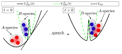
Figure 1: Schematic representation of the quench protocol consisting of (a) an initially tilted double-well with $V_{tilt}=dx>0$ to (b) a symmetric one with $V_{tilt}=d=0$. The quench leads to the tunneling dynamics of the two fermionic species being initially localized in the left well of their corresponding double-well. In the sketch the double-wells $V_{DW}^{A}$, $V_{DW}^{B}$ for each species are shown as well as the initial tilt $V_{tilt}$ (see legend).

To reveal the fragmented nature of each species we rely on the eigenvalues of the one-body reduced density matrix of the $\sigma$-species $\rho^{(1)}_{\sigma}(x,x^{\prime};t)=\bra{\Psi_{MB}(t)}\Psi^{\sigma\dagger}(x^{\prime})\Psi^{\sigma}(x)\ket{\Psi_{MB}(t)}$ Streltsov et al. (2008). The eigenfunctions of $\rho^{(1)}_{{\sigma}}(x,x^{\prime})$, are the so-called $\sigma$-species natural orbitals, $\phi^{\sigma}_{i}(x;t)$, which we consider to be normalized here to their corresponding eigenvalues $n^{\sigma}_{i}(t)=\int dx~{}\left|\phi^{\sigma}_{i}(x;t)\right|^{2}$. It can be shown that when $\Psi_{MB}(\vec{x}^{A},\vec{x}^{B};t)\to\Psi_{HF}(\vec{x}^{A},\vec{x}^{B};t)$ the corresponding natural populations obey $\sum_{i}^{N^{\sigma}}n_{i}^{\sigma}(t)=N_{\sigma}$, $n_{i>N_{\sigma}}^{\sigma}(t)=0$ and the corresponding Hartree-Fock wavefunction is retrieved. Therefore, if more than $N_{\sigma}$ natural orbitals are occupied, the system is said to be fragmented and the corresponding degree of fragmentation can be quantified via

$$F_{\sigma}(t)=N_{\sigma}-\sum\limits_{i=1}^{N_{\sigma}}n_{i}^{\sigma}(t).$$ (7)

This quantity serves as a theoretical measure for the occupation of the $m^{\sigma}-N_{\sigma}$ least occupied natural orbitals and thus for the deviation from a Hartree-Fock state when $F_{\sigma}>0$.

III Quench Induced Tunneling Dynamics

We consider a mass imbalanced repulsively interacting, $g_{AB}$, FF mixture consisting of $N_{A}=N_{B}=3$ fermions with $M_{A}=1$ and $M_{B}=6$. The system is initially prepared in the ground state of the tilted double-well described in Eq. (1) with tilt parameter $d=0.2$, frequency $\omega=0.1$, barrier height $V_{0}=1$ and width $w=1$. For these values and since $M_{B}>M_{A}$ the heavier B-species experiences a much more localized double-well around $x=0$ when compared to the double-well of the lighter A-species. Moreover due to the tilt, each species is found to be fully localized in its respective double-well, see Fig. 1 (a) for a schematic respresentation. Then the distinct fermionic clouds are non-overlaping for $t=0$, since $d=0.2$ see Fig. 2, and therefore phase separated at $x<0$. Concluding, this non-overlaping behavior between the two initial fermionic clouds is caused by their mass imbalance Shin et al. (2006, 2008) and renders the ground state to be essentially independent of $g_{AB}$, see Fig. 2. To examine the tunneling dynamics of the mass imbalanced FF mixture we perform a quench of the initially titled double-well with $d=0.2$ to a symmetric one i.e. $d=0$, see for instance Fig. 1 (b), keeping fixed all other parameters for a specific $g_{AB}$ and covering the regime from weak to strong interactions namely $g_{AB}\in[0,5]$.

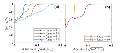
Figure 2: Ground state population, $\braket{\rho^{(1)}_{\sigma}}_{L}/N_{\sigma}$ [see also Eq. (4)], of the left well for each species for varying tilt $d$. Different particle numbers $N_{\sigma}$ and interspecies repulsions $g_{AB}$ are shown (see legend).

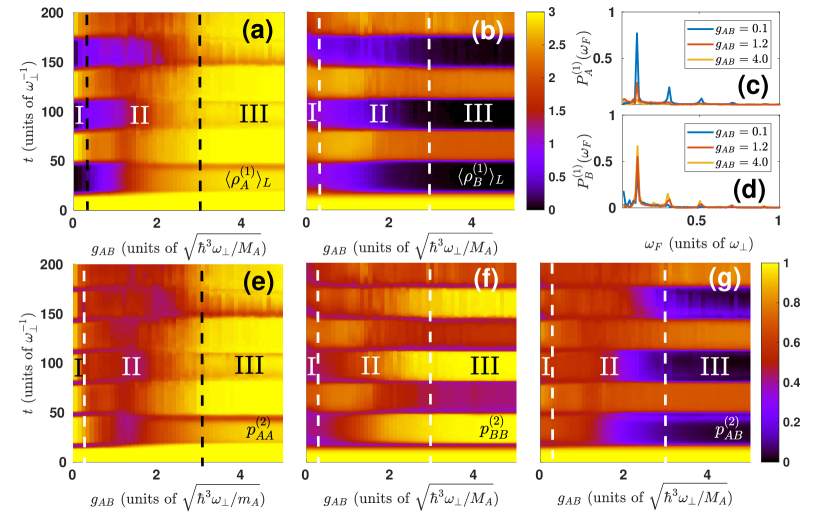
Figure 3: Time evolution of the expectation value of the one-body density in the left well, $\braket{\rho^{(1)}_{\sigma}(t)}_{L}$, of the (a) $\sigma=A$ and (b) $\sigma=B$ species for increasing interspecies repulsion $g_{AB}$. Fourier spectrum of (c) $\braket{\rho^{(1)}_{A}(t)}_{L}$ and (d) $\braket{\rho^{(1)}_{B}(t)}_{L}$ for different interspecies repulsions (see legends). Evolution of the two-body intraspecies probability, $p^{(2)}_{\sigma\sigma}(t)$, to find two fermions of the (e) $\sigma=A$ and (f) $\sigma=B$ species to reside in the same (either left or right) well for varying $g_{AB}$. (g) Interspecies two-body probability, $p^{(2)}_{AB}(t)$, for one fermion of each species to be within the same well for varying $g_{AB}$. In all cases the system consists of $N_{A}=N_{B}=3$ fermions initially confined in a tilted double-well with $d=0.2$ and we follow the tunneling dynamics after a quench to a symmetric double-well i.e. $d=0$.

III.1 One- and Two-Body Tunneling Probabilities

To monitor the overall tunneling dynamics on the one-body level for different values of $g_{AB}$ we rely on the expectation value of the single-particle density within the left well $\braket{\rho^{(1)}_{\sigma}(t)}_{L}$ [see also Eq. (4)] for each species. $\braket{\rho^{(1)}_{\sigma}(t)}_{L}$ essentially provides the percentage of the $\sigma$-species fermions within the left well or alternatively speaking the population imbalance between the two-sides of the double-well and offers therefore an adequate measure for the tunneling dynamics on the one-body level. Our primary aim is to investigate whether distinct tunneling regions for the fermions can be observed for a varying interspecies repulsion Sowiński et al. (2016). To conclude upon a certain tunneling regime we study $\braket{\rho^{(1)}_{\sigma}(t)}_{L}$ as well as its spectrum, $P^{(1)}_{\sigma}(\omega)=\operatorname{Re}\{\frac{1}{\pi}\int dt\braket{\rho^{(1)}_{\sigma}(t)}_{L}e^{i\omega t}\}$, in order to infer about the corresponding participating mode frequencies. Figures 3 (a) and (b) show $\braket{\rho^{(1)}_{A}(t)}_{L}$ and $\braket{\rho^{(1)}_{B}(t)}_{L}$ respectively for increasing $g_{AB}$. Inspecting $\braket{\rho^{(1)}_{\sigma}(t)}_{L}$ with respect to $g_{AB}$ we observe that the tunneling behavior of each species can be divided into three different regions denoted as I, II and III in Figs. 3 (a) and (b). Region I refers to weak interactions, namely $0<g_{AB}<0.2$, and the species $A$ ($B$) undergo a three (two)-mode tunneling motion, see also Figs. 3 (c), (d), where almost all fermions of each species oscillate back and forth between their left- and right wells Sowiński et al. (2016); Cao et al. (2017). Notice that $\braket{\rho^{(1)}_{\sigma}(t)}_{L}$ takes values between 0 and 3, see also Table 1. For increasing repulsion, $0.2<g_{AB}<3$, we enter region II where the tunneling process is modified with respect to region I, especially for the $A$-species. In particular the tunneling oscillations of the $A$- and $B$-species are characterized by one and two distinct frequencies respectively, see Figs. 3 (c) and (d). Regarding the tunneling behavior of the fermions this region can also be seen as a transition region between the weak and strong interaction regimes. For even stronger interactions $3<g_{AB}<5$, we realize region III where the $A$-species remains mainly in the left well, while the $B$-species still exhibits a strong amplitude two-frequency [see Figs. 3 (c), (d)] tunneling dynamics. As we shall argue below this latter interplay between the two species is caused by the fact that in this strongly interacting regime the heavier $B$-species acts as a material barrier for the lighter $A$-species, thus supressing the tunneling of the latter (see also Sec. III.3). Note also that for the $A$-species this region III is reminiscent to the few-body analogue of quantum self-trapping exhibited for strongly interacting bosons trapped in a double-well Chatterjee et al. (2010); Zöllner et al. (2008b, a, 2006a, 2006b). We actually observe a small amplitude tunneling for times $t>800$ (not shown here), while the observed tunneling amplitude of the $B$-species is even higher than in region I.

To gain deeper insights into the tunneling motion within and between the species and in order to reveal the underlying correlation mechanisms we invoke the pair probability $p_{\sigma\sigma\prime}^{(2)}(t)$ [Eq. (5)]. This quantity together with $\braket{\rho^{(1)}_{\sigma}(t)}_{L}$ enables us to identify the dominant particle configurations $\ket{N_{L},N_{R}}_{\sigma}$ occuring in the course of the dynamics. Here, $N_{L}$ ($N_{R}$) refers to the number of $\sigma$-species fermions in the left (right) well. We remark that due to the Pauli exclusion principle Giorgini et al. (2008); Pitaevskii and Stringari (2016) different fermions of the same species that reside in the same well populate energetically consecutive single-particle bands e.g. for $\ket{2,1}_{A}\equiv\ket{1^{0}\otimes 1^{1},1^{0}}$ where the upper index refers to the band number. The same holds for more than two fermions of different species that are in the same well. Referring to a certain time instant $t=t_{1}$ when e.g. $p_{AA}^{(2)}(t_{1})\approx 2/3$ and $2<\braket{\rho^{(1)}_{A}(t_{1})}_{L}<3$ the dominant $A$-species configuration corresponds to the superposition $\ket{2,1}_{A}+\ket{3,0}_{A}$. In the limiting case of $p_{AA}^{(2)}(t_{1})\approx 1$ and $\braket{\rho^{(1)}_{A}(t_{1})}_{L}\approx 3$ the $\ket{3,0}_{A}$ state is mainly contributing. It is also worth stressing at this point that in order to systematically conclude upon certain number state configurations one needs to rely on a projection of the numerically obtained many-body wavefunction to a multiband Wannier number state basis as it has been demonstrated in Mistakidis and Schmelcher (2017); Mistakidis et al. (2014, 2015a, 2015b); Koutentakis et al. (2017) e.g. for the single component bosonic case. However, such a numerical analysis in our FF mixture case is computationally challenging, since we need to take into account a large sample of number states in order to form a complete basis. Below we discuss the behavior of $p_{\sigma\sigma\prime}^{(2)}(t)$ within each of the above-mentioned tunneling regions I, II and III.

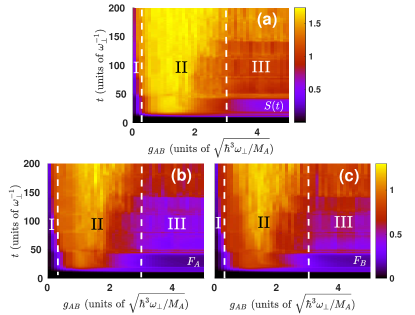
Figure 4: Time evolution of (a) the Von-Neumann entropy, $S(t)$, and the degree of fragmentation $F_{\sigma}(t)$ of the (b) $\sigma=A$ and (c) $\sigma=B$ species for increasing interspecies repulsion $g_{AB}$. The system consists of $N_{A}=N_{B}=3$ fermions prepared in a tilted double-well with $d=0.2$ which is subsequently quenched to a symmetric double-well i.e. $d=0$.

Region I	Region II	Region III
$0<g_{AB}<0.2$	$0.2<g_{AB}<3.0$	$3.0<g_{AB}<5.0$
$0<\braket{\rho^{(1)}_{A}}_{L}<3$	$0.9<\braket{\rho^{(1)}_{A}}_{L}<2.7$	$2.9<\braket{\rho^{(1)}_{A}}_{L}<3.0$
$1.0<\braket{\rho^{(1)}_{B}}_{L}<2.5$	$0.1<\braket{\rho^{(1)}_{B}}_{L}<2.7$	$0<\braket{\rho^{(1)}_{b}}_{L}<2.1$
$1.0<p^{(2)}_{AA}(t)<1.0$	$0.7<p^{(2)}_{AA}(t)<0.8$	$0.9<p^{(2)}_{AA}(t)<1.0$
$0.4<p^{(2)}_{BB}(t)<0.7$	$0.5<p^{(2)}_{BB}(t)<0.9$	$0.4<p^{(2)}_{BB}(t)<1.0$
$0.6<p^{(2)}_{AB}(t)<0.8$	$0.2<p^{(2)}_{AB}(t)<0.7$	$0<p^{(2)}_{AB}(t)<0.7$
$0<S(t)<0.8$	$0<S(t)<1.7$	$0<S(t)<1.4$
$0<F_{A}(t)<0.2$	$0<F_{A}(t)<1.1$	$0<F_{A}(t)<0.7$
$0<F_{B}(t)<0.2$	$0<F_{B}(t)<1.2$	$0<F_{B}(t)<0.8$

Table 1: Summary of the different tunneling regions of the FF mixture with respect to the interspecies interaction strength $g_{AB}$ and the corresponding range of the one- and two-body tunneling probabilities [$\braket{\rho^{(1)}_{\sigma}(t)}_{L}$, $p^{(2)}_{\sigma\sigma^{\prime}}(t)$], the Von-Neuman entropy $S(t)$ and the degree of fragmentantion $F_{\sigma}(t)$ for each species.

Regarding the $A$-species we observe that for both weak (region I) and strong interspecies interactions (region III) all three fermions reside in the same well since $p_{AA}^{(2)}(t)\approx 1$, see Fig. 3 (c) and also Table 1. The origin of the latter mechanism, in each region, can be better understood in combination with the corresponding behavior of $\braket{\rho^{(1)}_{A}(t)}_{L}$ [Fig. 3 (a)]. In particular, within the weak interaction regime (region I) all three particles perform a simultaneous tunneling from the left to the right-hand well and vice versa, since $\braket{\rho^{(1)}_{A}(t)}_{L}$ oscillates between 0 and 3. Then, the system predominantly oscillates between the configurations $\ket{3,0}_{A}$ and $\ket{0,3}_{A}$. However, for strong interactions (region III) the $A$-species fermions remain trapped in the left well as $2.9<\braket{\rho^{(1)}_{A}(t)}_{L}<3$ and the main contribution stems from the number state $\ket{3,0}_{A}$. In sharp contrast, within the intermediate interaction regime (region II) we observe that $0.7<p^{(2)}_{AA}(t)<0.8$ while $0.9<\braket{\rho^{(1)}_{A}(t)}_{L}<2.7$. As a consequence, at least one fermion tunnels from the left to the right well or better it is delocalized over both wells, see also Sec. III.3. This indicates that the states $\ket{2,1}_{A}$ and $\ket{1,2}_{A}$ dominantly contribute.

Next, we turn our attention to the dynamics of the $B$-species and show $p^{(2)}_{BB}(t)$ for varying $g_{AB}$ in Fig. 3 (d). As it can be seen $p^{(2)}_{BB}(t)$ differs significantly from $p^{(2)}_{AA}(t)$, see also Table 1. In region I, it oscillates between $p^{(2)}_{BB}\approx 1/3$ and $p^{(2)}_{BB}\approx 2/3$ while $1.0<\braket{\rho^{(1)}_{B}(t)}_{L}<2.5$ [Fig. 3 (b)]. Thus, the $B$-species cloud mainly tunnels between the $\ket{1,2}_{B}$ state (e.g. at $t\approx 30$) and the superposition $\ket{2,1}_{B}+\ket{3,0}_{B}$ (e.g. at $t\approx 60$) resulting in two and single particle tunneling respectively. In region II, $p^{(2)}_{BB}(t)$ exhibits small amplitude fluctuations around the value 0.7, while $0.1<\braket{\rho^{(1)}_{B}(t)}_{L}<2.7$. In this way, a unique assignment of number states is not possible since the $B$-species shows mainly a delocalized behavior over both wells. For completeness we should mention that the dynamics in region II is described by a higher-order superposition involving all available number states i.e. $\ket{3,0}_{B}$, $\ket{2,1}_{B}$, $\ket{0,3}_{B}$, $\ket{1,2}_{B}$. Entering region III, we can observe that the motion of the $B$-species alternates during the time evolution. Indeed, at the initial stages of the dynamics ($10<t<50$) all three $B$-species fermions tunnel to the right-hand well, see in particular that $p^{(2)}_{BB}(10<t<50)\approx 1$ and $\braket{\rho^{(1)}_{B}(10<t<50)}_{L}\approx 0$. For later time instants the cloud predominantly oscillates between $\ket{2,1}_{B}$ (e.g. $p^{(2)}_{BB}(t\approx 60)\approx 0.4$ and $\braket{\rho^{(1)}_{B}(t\approx 60)}_{L}\approx 2$) and $\ket{0,3}_{B}$ (e.g. $p^{(2)}_{BB}(t\approx 100)\approx 1$ and $\braket{\rho^{(1)}_{B}(t\approx 100)}_{L}\approx 0$). In this way we can infer that the fermions in this regime of interactions tunnel as pairs Chen et al. (2011); Meinert (2014); Mistakidis and Schmelcher (2017); Mistakidis et al. (2014).

To understand further the correlated dynamics within the different tunneling regions we additionally analyze the interspecies pair probability $p^{(2)}_{AB}(t)$ presented in Fig. 3 (e) and Table 1. Indeed within the region I $p^{(2)}_{AB}(t)$ undergoes small amplitude oscillations, see e.g. $p^{(2)}_{AB}(t\approx 30)\approx 2/3$ and $p^{(2)}_{AB}(t\approx 60)\approx 0.85$. The latter indicate that here the most significant number state configurations of the system correspond to the $\ket{0,3}_{A}\otimes\ket{1,2}_{B}$ and $\ket{3,0}_{A}\otimes\ket{2,1}_{B}+\ket{3,0}_{A}\otimes\ket{3,0}_{B}$ respectively. Turning to region II, $0.2<p^{(2)}_{AB}(t)<0.7$ and therefore a clear assignment in terms of number states can not be unavoided. However this suggests, as it has already been observed in $p^{(2)}_{AA}(t)$ and $p^{(2)}_{BB}(t)$, the participation of a multitude of number states and as a result the occurrence of a multimode dynamics. Is is also worth stressing again that this interaction regime II exhibits a strongly alternating behavior with respect to $g_{AB}$ , e.g. see $\braket{\rho^{(1)}_{\sigma}(t)}_{L}$, $p^{(2)}_{\sigma\sigma^{\prime}}(t)$ for $0.2<g_{AB}<1.7$ and $1.7<g_{AB}<3.0$ in Fig. 3. Moreover, as we shall argue below the dynamics in this region is characterized by an enhanced degree of both entanglement and fragmentation, see Sec. III.2. Finally, for strong interactions (region III) $p^{(2)}_{AB}(t)$ shows a much more pronounced oscillatory pattern when compared to regions I and II. Since here the $A$-species is fully trapped in the left well this behavior of $p^{(2)}_{AB}(t)$ is attributed to the motion of the $B$-species which perform pair tunneling, i.e. $\ket{2,1}_{B}\leftrightarrow\ket{0,3}_{B}$.

III.2 Entanglement and Fragmentation

To expose the many-body nature of the dynamics of the FF mixture we next measure the degree of entanglement (or interspecies correlations) and the fragmentation (or intraspecies correlations) of the underlying many-body state. These features can be quantified by employing $S(t)$ and $F_{\sigma}(t)$ respectively for varying $g_{AB}$, see Fig. 4 and Table 1. We remind here that when $S(t)=0$ the system is called non-entangled, while $S(t)\neq 0$ signifies the presence of entanglement or interspecies correlations. Accordingly, for $F_{\sigma}(t)>0$ the $\sigma$-species is termed intraspecies correlated (see also Sec. II.3). Most importantly, since the fermions of each species are spin-polarized, i.e. non-interacting, the occurrence of intraspecies correlations during the evolution is induced by the interspecies correlations. Recall also that in the initial (ground) state of the system the distinct fermionic clouds that reside in the left well, see Fig. 1 (a), are non-overlaping and therefore fully phase separated due to their mass imbalance Shin et al. (2006, 2008). Due to this non-overlaping behavior no inter- and intraspecies correlations occur for arbitrary $g_{AB}$. As it can be easily seen in Figs. 4 (a), (b), (c) for weak interactions (region I) there is only a small amount of inter- and intraspecies correlations since both $S(t)$ and $F_{\sigma}(t)$ are suppressed. Strikingly enough, for intermediate interactions (region II) $S(t)$ as well as $F_{\sigma}(t)$ increase during the evolution and tend to saturate to a certain finite value, signifying that the many-body state is strongly entangled and fragmented. Inspecting region III we observe again that both $S(t)$ and $F_{\sigma}(t)$ increase in the course of time but in a slower manner as compared to region II. Also they acquire moderate magnitudes with respect to region II. Interestingly enough within this strongly interacting regime III, $F_{B}(t)$ (heavier species) increases more rapidly during the evolution when compared to $F_{A}(t)$ (lighter species).

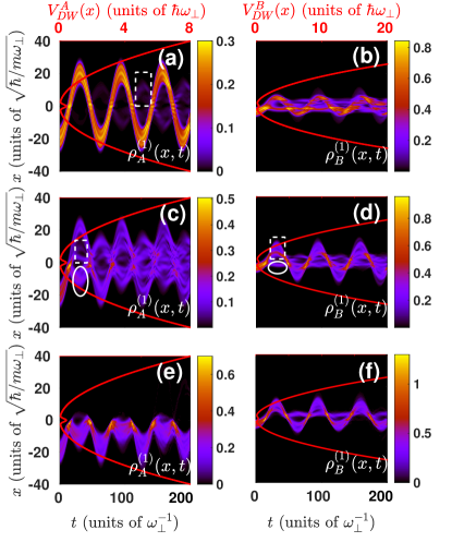
Figure 5: Evolution of the single-particle density for the $A$ (left column) and the $B$-species (right column) of a FF mixture consisting of $N_{A}=N_{B}=3$ fermions after a quench of the tilt parameter from $d=0.2$ to $d=0$. The interspecies interaction corresponds to (a), (b) $g_{AB}=0.1$, (c), (d) $g_{AB}=1.2$ and (e), (f) $g_{AB}=4$ respectively. The dashed rectangles and solid ellipses indicate the fermionic fragments that tunnel and are reflected back respectively due to the barrier or a collision with the other species. The double-well that each species experiences, $V_{DW}^{\sigma}$, is also shown on top of the density evolution.

III.3 Single-Particle Density Evolution

To visualize the tunneling motion in the different interaction regimes identified above, we finally invoke the evolution of the single-particle density, $\rho^{(1)}_{\sigma}(t)$, for each of the species see Fig. 5. Due to its larger mass the $B$-species resides near the barrier, while the lighter $A$-species is in comparison shifted to the left. Within the region I, see Figs. 5 (a) and (b), the $A$-species cloud oscillates as a whole back and forth resulting in a three-body tunneling process. Only for large evolution times, $t>100$, a small fraction of the $A$-species gets reflected from the barrier, see the dashed rectangle in Fig. 5 (a). For the $B$-species a substantial reflection already occurs during the first tunneling process and a corresponding fraction remains trapped in the left well. Consequently a delocalization of $\rho^{(1)}_{B}(t)$ takes place. At intermediate interspecies interactions (region II) both species (and especially the lighter $A$-species) are reflected from both the barrier as well as from the other species, see Figs. 5 (c), (d). In particular, during the initial stages of the dynamics ($0<t<25$) both the $A$- and the $B$-species travel towards the barrier where they split into two fragments from which one tunnels through the barrier to the right well [see the dashed rectangles in Figs. 5 (c), (d)] and the other one is reflected back to the left well [see the solid ellipses in Figs. 5 (c), (d)]. Then, the transmitted fragments of the $A$- and the $B$-species collide in the right well [see e.g. the dashed rectangle in Fig. 5 (c)]. As a result a further split into two new fragments takes place. One of these fragments travels back to the barrier and the other one continues towards the outer part of the right well. The effect of this collisional dynamics is, of course, much more pronounced for the $A$-species since it is the lighter one Krönke et al. (2013) and it is manifested by the delocalization of both species over the wells. This delocalization becomes even more apparent for large evolution times, $t>100$, and it is a consequence of the fact that the distinct species suffer multiple collisions with one another, rendering the one-body density blurred. Recall also that the dynamics in this regime of interactions is strongly entangled and fragmented, see Fig. 4. Let us also comment at this point that within the Hartree-Fock approximation the above-mentioned delocalization of both species during the evolution becomes suppressed (not shown here for brevity) since it is essentially caused by the contribution of the higher-lying orbitals. Turning to the strongly interacting regime (region III), we observe that the heavier $B$-species acts as a hard-wall or material barrier for the lighter $A$-species Pflanzer et al. (2009, 2010), as shown in Figs. 5 (e), (f). In this way, the $A$-species remains fully trapped within the left well during the evolution, while the $B$-species still performs a tunneling motion. The only effect of the collision between the two species that is imprinted in the density of the $B$-species is a splitting of its density into two parts, one of which undergoes tunneling between the two wells and the other remains trapped in the right well where it performs tiny amplitude oscillations.

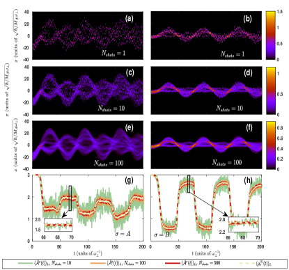
Figure 6: Averaged images over (a), (b) $N_{shots}=1$, (c), (d) $N_{shots}=10$, (e), (f) $N_{shots}=100$. (g), (h) Evolution of $\braket{\rho^{(1)}_{\sigma}(t)}_{L}$ and the probabilities, $\braket{\bar{\mathcal{A}}^{\sigma}(t)}$, obtained by averaging several single-shot images (see legend). The insets illustrate $\braket{\bar{\mathcal{A}}^{\sigma}(t)}$ in certain time intervals. In all cases the system consists of $N_{A}=N_{B}=3$ fermions with $M_{B}/M_{A}=6$ and $g_{AB}=1.2$, while the dynamics is induced by performing a quench of the initially tilted double-well ($d=0.2$) to a symmetric one with $d=0$. Left panels indicate the $A$-species and right panels refer to the $B$-species.

IV Single-Shot Simulations

To provide possible experimental evidence for the many-body tunneling dynamics of the FF mixture we simulate in-situ single-shot absorption measurements Sakmann and Kasevich (2016); Mistakidis et al. (2018); Lode and Bruder (2017). This type of measurements probe the spatial configuration of the atoms which can be inferred by the many-body probability distribution. Such experimental images refer to a convolution of the spatial particle configuration with a point spread function which essentially dictates the corresponding experimental resolution. For our calculations, to be presented below, we use a point spread function of Gaussian shape possessing a width $w_{PSF}=1\ll l\approx 3.2$, where $l=\sqrt{1/\omega}$ denotes the corresponding harmonic oscillator length. It is also important to note here that in few-body experiments Zürn et al. (2012); Wenz et al. (2013) besides the in-situ imaging of the cloud another technique to probe the state of the system and get rid of unavoidable noise sources that might destroy the experimental signal is fluorescence imaging Serwane et al. (2011); Koutentakis et al. (2018). However, the simulation of this technique which has been proven important for few-body experiments lies beyond our current scope. Here we aim at demonstrating how in-situ imaging can be used to adequately monitor the above-described few-body FF mixture dynamics.

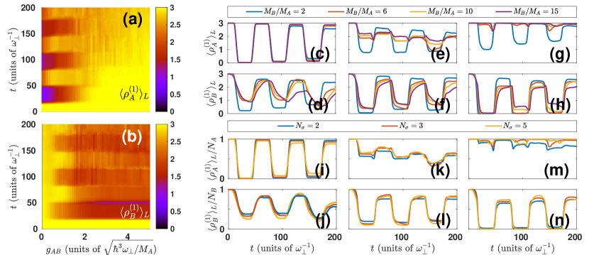
Figure 7: Evolution of $\braket{\rho^{(1)}_{\sigma}(t)}_{L}$, of the (a) $\sigma=A$ and (b) $\sigma=B$ species with mass ratio $M_{B}/M_{A}=6$ residing in a double-well with barrier height $V_{0}=4$, for increasing interspecies repulsion $g_{AB}$. (c)-(h) $\braket{\rho^{(1)}_{\sigma}(t)}_{L}$ for different mass ratios (see legend) and interspecies repulsion (c), (d) $g_{AB}=0.1$, (e), (f) $g_{AB}=1.5$ and (g), (h) $g_{AB}=4.0$. (a)-(h) The system consists of $N_{A}=N_{B}=3$ fermions. (i)-(n) $\braket{\rho^{(1)}_{\sigma}(t)}_{L}/N_{\sigma}$ for varying number of fermions (see legend) with $M_{B}/M_{A}=6$ and interspecies repulsion (i), (j) $g_{AB}=0.1$, (k), (l) $g_{AB}=1.5$ and (m), (n) $g_{AB}=4.0$. The corresponding barrier height of the double-well in (c)-(n) is $V_{0}=1$. In all cases the FF mixture is initially confined in a tilted double-well with $d=0.2$ and the dynamics is induced by quenching to a symmetric double-well i.e. $d=0$.

Relying on the system’s many-body wavefunction obtained within ML-MCTDHX we simulate in-situ single shot images for both species $A$, $\mathcal{A}^{A}(\tilde{x};t)$, and species $B$, $\mathcal{A}^{B}(\tilde{x^{\prime}}|\mathcal{A}^{A}(\tilde{x});t_{im})$, at each instant $t$ of the evolution when we consecutively image first the $A$ and then the $B$ species. For details regarding the simulation process of this experimental technique we refer to Appendix B. Below we focus on the FF dynamics, possessing $g_{AB}=1.2$ (region II), within the double-well upon quenching the tilt parameter from $d=0.2$ to $d=0$. Note that a similar procedure has been followed also for other values of $g_{AB}$ (not shown here). Figures 6 ($a$), ($b$) show the first simulated in-situ single-shot images for both species during the evolution, namely $\mathcal{A}^{A}(\tilde{x};t)$, and $\mathcal{A}^{B}(\tilde{x^{\prime}}|\mathcal{A}^{A}(\tilde{x});t)$ respectively. It can be deduced that the two species exhibit a tunneling behavior, resembling this way the overall tendency observed in the one-body density [see also Figs. 5 (c), (d)]. However, it is important to mention that a direct correspondence between the one-body density and one single-shot image is not possible due to the small particle number of the considered FF mixture, $N_{A}=N_{B}=3$. Another source of the inability to explicitly observe the one-body density within a single-shot image is the presence of multiple orbitals in the system. Indeed, the many-body state builds upon a superposition of multiple orbitals [see Eqs. (2) and (3)] and therefore imaging an atom alters the many-body state of the other atoms and hence their one-body density. For a more elaborated discussion on this topic see Mistakidis et al. (2018); Katsimiga et al. (2017a, 2018). To retrieve the one-body density of the system we next rely on an average of several single-shot images for each species, namely $\bar{\mathcal{A}}^{A}(\tilde{x};t)=1/N_{shots}\sum_{k=1}^{N_{shots}}\mathcal{A}_{k}^{A}(\tilde{x};t)$ and $\bar{\mathcal{A}}^{B}(\tilde{x}^{{}^{\prime}}|\mathcal{A}^{A}(\tilde{x});t)=1/N_{shots}\sum_{k=1}^{N_{shots}}\mathcal{A}_{k}^{B}(\tilde{x}^{{}^{\prime}}|\mathcal{A}^{A}(\tilde{x});t)$ respectively. In particular, Figs. 6 (c)-(f) illustrate $\bar{\mathcal{A}}^{A}(\tilde{x};t)$ and $\bar{\mathcal{A}}^{B}(\tilde{x}^{{}^{\prime}}|\mathcal{A}^{A}(\tilde{x});t)$ for different number of samplings i.e. $N_{shots}$. Evidently, a comparison of this averaging process for an increasing number of shots and the actual one-body density obtained within ML-MCTDHX [see Figs. 5 (c), (d)] reveals that they are almost identical. Namely as the number of shots, $N_{shots}$, becomes larger then $\bar{\mathcal{A}}^{A}(\tilde{x};t)$ and $\bar{\mathcal{A}}^{B}(\tilde{x}^{{}^{\prime}}|\mathcal{A}^{A}(\tilde{x});t)$ tend gradually to $\rho^{(1)}_{A}(t)$ and $\rho^{(1)}_{B}(t)$ respectively. To further support our above-mentioned arguments we finally contrast the one-body tunneling probabilities $\braket{\rho^{(1)}_{A}(t)}_{L}$ and $\braket{\rho^{(1)}_{B}(t)}_{L}$ at $g_{AB}=1.2$ with the corresponfing simulated and experimentally to be observed probabilities i.e. $\braket{\bar{\mathcal{A}}^{A}(t)}=\int_{\tilde{x}<0}d\tilde{x}\bar{\mathcal{A}}^{A}(\tilde{x};t)$ and $\braket{\bar{\mathcal{A}}^{B}(t)}=\int_{\tilde{x}^{{}^{\prime}}<0}d\tilde{x}^{{}^{\prime}}\bar{\mathcal{A}}^{B}(\tilde{x}^{{}^{\prime}}|\mathcal{A}^{A}(\tilde{x});t)$ [see Figs. 6 (g), (h)]. As it can be readily seen, a larger number of $N_{shots}$, see in particular the insets in Figs. 6 (g), (h), (here $N_{shots}>100$) reproduces almost perfectly both $\braket{\rho^{(1)}_{A}(t)}_{L}$ and $\braket{\rho^{(1)}_{B}(t)}_{L}$, capturing this way the tunneling process.

V Further Characteristics of the Tunneling Dynamics

Having discussed in detail the properties of the tunneling dynamics of the FF mixture in the double-well, we finally showcase how the overall dynamics depends on certain system parameters. To this end, we first study the effect of the barrier height $V_{0}$ on the quench induced tunneling dynamics. As a reference system we consider the double-well with $V_{0}=1$ that has already been discussed above, while as an indicator for the tunneling dynamics we employ $\braket{\rho^{(1)}_{\sigma}(t)}_{L}$. Figures 7 (a), (b) present $\braket{\rho^{(1)}_{A}(t)}_{L}$ and $\braket{\rho^{(1)}_{B}(t)}_{L}$ respectively for the case $V_{0}=4$ for varying interspecies repulsion $g_{AB}$. We observe that the tunneling dynamics of both species, and especially the $B$-species, is strongly influenced by the barrier height and in particular it is overall suppressed Mistakidis et al. (2015a); Sowiński et al. (2016); Fasshauer and Lode (2016), compare Figs. 3 (a), (b) and Figs. 7 (a), (b). Regarding the $A$-species the three above-identified tunneling regions are shifted to weaker interactions and in particular region I becomes negligible in size and exists only very close to the non-interacting limit [hardly visible in Fig. 7 (a)]. Therefore, an increasing barrier height shows a similar effect on the $A$-species as a stronger interaction strength where the $B$-species acts as a material barrier Pflanzer et al. (2009, 2010), see for instance Fig. 5 (e). For the heavier $B$-species the barrier height has the most prominent effect as the tunneling dynamics is significantly suppressed for every value of $g_{AB}$ when compared to the $V_{0}=1$ case where tunneling oscillations occur independently of the interaction strength. Here the tunneling takes place for $g_{AB}>1$ and it exhibits a small amplitude.

As a next step, we examine the influence of the mass ratio on the tunneling behavior of the FF mixture by inspecting again $\braket{\rho^{(1)}_{\sigma}(t)}_{L}$ within the different interaction regimes. Since a mass ratio $M_{B}/M_{A}>15$ leads to a ground state where both species are not fully trapped in the left well for an initial tilt magnitude $d=0.2$, we investigate below only imbalances that satisfy $M_{B}/M_{A}\in[2,15]$. In particular we show $\braket{\rho^{(1)}_{\sigma}(t)}_{L}$ in each of the regions I, II and III for $M_{B}/M_{A}\in\{2,6,10,15\}$, see Figs. 7 (c)-(h). Referring to weak interactions, see Figs. 7 (c), (d), we observe that an increasing mass ratio mainly affects the heavier $B$-species. Indeed, the amplitude of $\braket{\rho^{(1)}_{B}(t)}_{L}$ is reduced for a larger $M_{B}$, accompanied by an overall damping in the course of time. In contrast $\braket{\rho^{(1)}_{A}(t)}_{L}$ is essentially independent of the increasing $M_{B}$ with the only noticeable difference being a slight lowering of the damping amplitude of the $\braket{\rho^{(1)}_{A}(t)}_{L}$ oscillation for sufficiently large evolution times. Turning to intermediate interactions (region II) we deduce that the oscillation amplitude of $\braket{\rho^{(1)}_{\sigma}(t)}_{L}$ decreases during evolution while its damping increases for both species for increasing mass ratios, see Figs. 7 (e), (f). This damping behavior is much stronger for the lighter $A$-species as it be seen by comparing Figs. 7 (e) and (f). Interestingly enough, an irregular behavior of $\braket{\rho^{(1)}_{B}(t)}_{L}$ takes place at the turning points of the tunneling motion with a tendency to a sawtooth waveform. For strong interspecies interactions (region III) the tunneling dynamics of the $A$-species vanishes for larger $M_{B}$. However, the $B$-species exhibits prominent tunneling oscillations which show a damping behavior for increasing $M_{B}$. Indeed, according to our observations for strong $g_{AB}$ in the case of $M_{B}/M_{A}=6$ [Figs. 5 (e), (f)] the heavier $B$-species acts as an effective material barrier Pflanzer et al. (2009, 2010) for the lighter $A$-species and its collision with the $B$-species pushes the latter to the right well, enforcing its tunneling motion.

To shed light on the particle number dependence of the tunneling motion, we finally utilize the normalized expectation value $\langle\rho_{\sigma}^{(1)}(t)\rangle_{L}/N_{\sigma}$ for a varying particle number $N_{\sigma}\in\{2,3,5\}$ within the different interaction regimes, see Figs. 7 (i)-(n). Overall, we observe that for all three interaction regimes (I, II, III) an increasing particle number results in a stronger damping of $\langle\rho_{\sigma}^{(1)}(t)\rangle_{L}/N_{\sigma}$ for the lighter $A$-species, while the corresponding damping of the heavier $B$-species is washed out. All the other one-body tunneling features, e.g. the frequency and the amplitude of the $\langle\rho_{\sigma}^{(1)}(t)\rangle_{L}/N_{\sigma}$ oscillation, remain essentially insensitive. An inspection of the two-body tunneling characteristics unveils more pronounced differences since for larger particle numbers more modes are triggered which are imprinted e.g. in the $p^{(2)}_{\sigma\sigma^{\prime}}$ evolution (results not shown here).

VI Conclusions

We have investigated the tunneling dynamics of a FF mixture with spin polarized components confined in a double-well. The fermionic mixture is initially prepared within the left well of a tilted double-well and the tunneling dynamics is induced by removing the tilt and let the system evolve in a symmetric double-well. We particularly examined the impact of the interspecies interactions on the tunneling behavior of each species and unveiled the significant role of intra- and interspecies correlations. The emergent dynamics has been characterized on both the one- and two-body level by invoking the single- and two-particle probabilities for the fermions of each species to reside e.g. in the left-hand well in the course of the dynamics.

For very weak interactions close to the non-interacting limit both species perform almost perfect Rabi-oscillations. The heavier species exhibit small deviations from the perfect Rabi scenario since they either show single or two-particle tunneling i.e. during the evolution not all three particles tunnel together. Increasing the interspecies repulsion the tunneling dynamics is suppressed for both species. The lighter species undergoes single-particle tunneling, while for the heavier one a more complex dynamics takes place which is characterized by a higher-order quantum superposition further indicating the presence of strong correlations in the system. Turning to strong interactions we observe that the lighter species experiences a quantum self-trapping due to the heavier species which acts as a material barrier. In particular, the collision between the two species causes a splitting of the density of the heavier component into two parts. The first part performs tunneling between the two wells and the other one remains trapped in the right well exhibiting small amplitude oscillations. As a consequence, this heavier component undergoes almost perfect Rabi-oscillations being characterized either by three-particle or pair tunneling at different instants of the evolution. The degree of both inter- and intraspecies correlations for all interaction regimes has been exposed and found to be overall significant especially for intermediate interactions. To relate our findings with possible experimental realizations we simulate in-situ single-shot measurements and showcase how an increasing sampling of such images can be used to adequately reproduce the observed fermionic tunneling dynamics.

The dependence of the observed tunneling behavior on the mass ratio of the two components, the particle number and the height of the barrier of the double-well has been discussed. It is shown that the mass imbalance between the components possesses a strong influence on the tunneling dynamics depending on the interspecies interaction strength. Namely, for weaker interactions the tunneling amplitude of the heavier species becomes smaller for an increasing mass ratio, while the tunneling features of the lighter species remain essentially unaffected. Increasing the repulsion a decrease of the tunneling amplitude for both species occurs during evolution. For strong interactions the heavier species acts as a material barrier for the lighter one thus suppressing the tunneling motion of the latter. On the other hand, for fixed interspecies repulsion and larger particle numbers a damping of the tunneling oscillations takes place especially for the lighter species. Finally, we show that for a higher barrier the tunneling dynamics of both species, and in particular of the heavier one, is overall suppressed since an increasing barrier disfavors the tunneling process.

There is a multitude of interesting directions worth pursuing in future studies. A straightforward one would be to examine the tunneling dynamics of a dipolar FF mixture, under the quench protocol considered herein, and investigate how the long-range character of the interactions alters the emergent tunneling behavior including the inherent entanglement generation. Another interesting prospect is to unravel the collisional dynamics of two fermi components which are initially well separated, e.g. due to the presence of a high barrier and then are left to collide by removing this intermediate barrier in a sense of the counterflow experiment. Inspecting the many-body character of the spontaneously generated non-linear excitations such as dark solitons Scott et al. (2011) or domain-wall structures Katsimiga et al. (2017a, 2018) between the two species is a challenging future task. Finally, the generalization of our current findings utilizing time-dependent quench protocols would be desirable in order to design schemes for selective transport between the wells of each component.

Appendix A Tunneling Dynamics Versus Energy Offset

Let us briefly comment on the influence of the quench strength, i.e. the value of the postquench tilt parameter $d$, on the tunneling dynamics of both species of the FF mixture. We consider a FF mixture of $N_{A}=N_{B}=3$ with $M_{B}/M_{A}=6$ and $g_{AB}=0.1$ trapped initially in a tilted double-well with $d=0.2$ and $h=1$. To induce the tunneling dynamics we perform a quench to a smaller value of the tilt $d\in[0,0.2)$, thus rendering the energy offset between the wells smaller and favoring the tunneling motion of both species from the left to the right well.

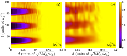
Figure 8: $\braket{\rho^{(1)}_{\sigma}(t)}_{L}$, of the (a) $\sigma=A$ and (b) $\sigma=B$ species for varying postquench tilt parameter $d$. The mixture consists of $N_{A}=N_{B}=3$ fermions repulsively interacting with $g_{AB}=0.1$ and $M_{B}/M_{A}=6$ and being initially trapped in a tilted double-well with $d=0.2$ and $V_{0}=1$. The dynamics is induced by a quench on the tilt parameter $d$.

Figures 8 (a), (b) present $\braket{\rho^{(1)}_{\sigma}(t)}_{L}$ for a varying postquench amplitude of the tilt magnitude $d$. For offsets characterized by $0<d<0.03$ we do not observe any significant influence on the tunneling oscillations of both species. Entering the region $0.03<d<0.09$ significant alterations in $\braket{\rho^{(1)}_{\sigma}(t)}_{L}$ occur in the sense that the oscillation frequency and amplitude decrease for a larger offset. Finally, for $d>0.09$ both species remain in the left well without tunneling throughout the evolution as the energy offset is adequately large and suppresses any possible tunneling process. We remark that we have performed the same investigation for both intermediate and strong interspecies interactions $g_{AB}$, observing a similar behavior of the emerging dynamics within the same postquench intervals of the tilt magnitude $d$ as above (not shown here for brevity).

Appendix B Single-Shots Implementation in Fermi-Fermi Mixtures

To simulate the experimental single-shot procedure we perform a sampling of the many-body probability distribution Sakmann and Kasevich (2016); Katsimiga et al. (2017a, 2018); Mistakidis et al. (2018) being accessible within the ML-MCTDHX framework. We remark that such a theoretical implementation of the experimental process has already been performed for single-species bosons Sakmann and Kasevich (2016); Lode and Bruder (2017); Katsimiga et al. (2017a, 2018) and fermions Koutentakis et al. (2018) as well as for binary bosonic ensembles Mistakidis et al. (2018) but not yet for FF mixtures. As in the two-species bosonic case, the corresponding single-shot procedure for FF mixtures depends strongly on the inter- and intraspecies correlations inherent in the system. Indeed within a many-body treatment the presence of entanglement between the different species is of significant importance regarding the image ordering. This can be understood by inspecting the Schmidt decomposition [see Eq. (2)] and especially the involved Schmidt coefficients $\lambda_{k}$’s. Below let us elaborate on the corresponding process where we image first the $A$ and then the $B$-species, obtaining in this way the images $\mathcal{A}^{A}(\tilde{x})$ and $\mathcal{A}^{B}(\tilde{x^{\prime}}|\mathcal{A}^{A}(\tilde{x}))$. However, we note that the same overall procedure has to be followed in order to image first the $B$ and then the $A$ species, resulting in single-shots images $\mathcal{A}^{B}(\tilde{x})$ and $\mathcal{A}^{A}(\tilde{x^{\prime}}|\mathcal{A}^{B}(\tilde{x}))$ respectively.

To image first the $A$ and then the $B$ species we consecutively annihilate all the $N_{A}$ fermions. Referring to a specific time instant of the imaging process, e.g. $t_{im}$, a random position is drawn that satisfies the constraint $\rho_{N_{A}}^{(1)}(x_{1}^{\prime})>q_{1}$, where $q_{1}$ denotes a random number lying in the interval [$0$, $\max\{{\rho^{(1)}_{N_{A}}(x;t_{im})\}}$]. Next, we project the ($N_{A}+N_{B}$)-body wavefunction onto the ($N_{A}-1+N_{B}$)-body one. The latter is accomplished by the use of the projection operator $\frac{1}{\mathcal{N}}(\hat{\Psi}_{A}(x_{1}^{\prime})\otimes\hat{\mathbb{I}}_{B})$, where $\hat{\Psi}_{A}(x_{1}^{\prime})$ refers to the fermionic field operator that annihilates an $A$ species fermion located at $x_{1}^{\prime}$ and $\mathcal{N}$ is the normalization constant. An important observation, here, is that the above process affects the Schmidt weights, $\lambda_{k}$, and therefore besides that the $B$-species has not already been imaged, both $\rho^{(1)}_{N_{A}-1}(t_{im})$ and $\rho^{(1)}_{N_{B}}(t_{im})$ are altered. To comprehend the latter we rely on the Schmidt decomposition according to which the many-body wavefunction after the first measurement reads

$$\begin{split}&\ket{\tilde{\Psi}_{MB}^{N_{A}-1,N_{B}}(t_{im})}=\\ &\sum_{i}\sqrt{\tilde{\lambda}_{i,N_{A}-1}(t_{im})}\ket{\tilde{\Psi}_{i,N_{A}-1}^{A}(t_{im})}\ket{\Psi_{i}^{B}(t_{im})}.\end{split}$$ (8)

In this expression, $\ket{\tilde{\Psi}_{i,N_{A}-1}^{A}}=\frac{1}{N_{i}}\hat{\Psi}_{A}(x_{1}^{\prime})\ket{\Psi_{i}^{A}}$ denotes the $N_{A}-1$ species wavefunction, $N_{i}=\sqrt{\bra{\Psi_{i}^{A}}\hat{\Psi}_{A}^{\dagger}(x_{1}^{\prime})\hat{\Psi}_{A}(x_{1}^{\prime})\ket{\Psi_{i}^{A}}}$ is the normalization factor and $\tilde{\lambda}_{i,N_{A}-1}=\lambda_{i}N_{i}/\sum_{i}\lambda_{i}N_{i}^{2}$ refer to the Schmidt coefficients of the ($N_{A}-1+N_{B}$)-body wavefunction. Repeating the above steps $N_{A}-1$ times we obtain the following distribution of positions ($x^{\prime}_{1}$, $x^{\prime}_{2}$,…,$x^{\prime}_{N_{A}-1}$) which is then convoluted with a point spread function. This results in the single-shot image $\mathcal{A}^{A}(\tilde{x})=\sum_{i=1}^{N_{A}}e^{-\frac{(\tilde{x}-x^{\prime}_{i})^{2}}{2w_{PSF}^{2}}}$ for the $A$-species, where $\tilde{x}$ are the spatial coordinates within the image and $w_{PSF}$ is the width of the employed point spread function. It is also important to mention at this point that after annihilating all $A$-species fermions the many-body wavefunction reads

$$\begin{split}&\ket{\tilde{\Psi}_{MB}^{0,N_{B}}(t_{im})}=\\ &\ket{0}\otimes\sum_{i}\frac{\sqrt{\tilde{\lambda}_{i,1}(t_{im})}\braket{x}{\Phi_{i,1}^{A}}}{\sum_{j}{\sqrt{\tilde{\lambda}_{j,1}(t_{im})|\braket{x}{\Phi_{j,1}^{A}}|^{2}}}}\ket{\Psi_{i}^{B}(t_{im})},\end{split}$$ (9)

where $\braket{x}{\Phi_{j,1}^{A}}$ refers to the single-particle orbital of the $j$-th mode and the wavefunction of the $B$-species, $\ket{\Psi_{MB}^{N_{B}}(t_{im})}$, corresponds to the second term of the cross product on the right-hand side. Evidently, $\ket{\Psi_{MB}^{N_{B}}(t_{im})}$ obtained after the annihilation of all $N_{A}$ fermions corresponds to a non-entangled $N_{B}$-particle many-body wavefunction and its corresponding single-shot procedure reduces to that of the single-species case Sakmann and Kasevich (2016); Katsimiga et al. (2017a, 2018). The latter has been extensively used in a variety of settings (see e.g. Sakmann and Kasevich (2016); Katsimiga et al. (2017a, 2018)) and therefore it is only briefly outlined below. For a time instant of the imaging $t=t_{im}$ we calculate $\rho^{(1)}_{N_{B}}(x;t_{im})$ from the many-body wavefunction $\ket{\Psi_{N_{B}}}\equiv\ket{\Psi(t_{im})}$. Next, a random position $x^{\prime\prime}_{1}$ is drawn according to the constraint $\rho^{(1)}_{N_{B}}(x^{\prime\prime}_{1};t_{im})>q_{2}$, with $q_{2}$ being a random number within [$0$, $\rho^{(1)}_{N_{B}}(x;t_{im})$]. Then, one particle at position $x^{\prime\prime}_{1}$ is annihilated and the $\rho^{(1)}_{N_{B}-1}(x;t_{im})$ is calculated from $\ket{\Psi_{N_{B}-1}}$. To proceed, a new random position $x^{\prime\prime}_{2}$ is drawn from $\rho^{(1)}_{N_{B}-1}(x;t_{im})$. We repeat this procedure for $N_{B}-1$ steps and obtain the distribution of positions ($x^{\prime\prime}_{1}$, $x^{\prime\prime}_{2}$,…,$x^{\prime\prime}_{N_{B}-1}$) which is then convoluted with a point spread function leading to a single-shot image $\mathcal{A}^{B}(\tilde{x^{\prime}}|\mathcal{A}^{A}(\tilde{x}))$.

Appendix C Remarks on Convergence of the Many-Body Simulations

Let us finally briefly discuss the basic aspects of our numerical method and then showcase the convergence of our results. ML-MCTDHX Krönke et al. (2013) consists of a variational method for solving the time-dependent many-body Schrödinger equation of atomic mixtures with constituents being either of Bose Mistakidis et al. (2018); Katsimiga et al. (2017b) or Fermi Cao et al. (2017); Koutentakis et al. (2018) type. To construct the many-body wavefunction a time-dependent variationally optimized many-body basis is employed, enabling us to take into account the system’s important correlation effects using a computationally feasible basis size. Therefore the system’s relevant subspace of the Hilbert space is spanned at each time instant of the evolution in a more efficient manner when compared to expansions relying on a time-independent basis as the number of basis states can be significantly reduced. Finally, as a result of the multi-layer ansatz for the total wavefunction we are able to capture both the intra- and the interspecies correlations emerging during the non-equilibrium dynamics of a bipartite system.

Figure 9: Evolution of the deviations $\Delta\langle\rho^{(1)}_{\sigma;C,C^{\prime}}(t)\rangle_{L}$ between the $C^{\prime}=9-(9,9)$ and other numerical configurations $C=M-(m^{A},m^{B})$ (see legends) for (a), (c) $g_{AB}=1.2$ and (b), (d): $g_{AB}=4.0$. The particle number of each component is $N_{A}=N_{B}=3$.

Within our approach the used Hilbert space truncation, namely the order of the considered approximation, corresponds to the employed numerical configuration space being denoted by $C=M-(m^{A},m^{B})$. In this notation $M=M^{A}=M^{B}$ and $m^{A}$, $m^{B}$ refer to the number of species and single-particle functions respectively for each of the species. We also note that for our simulations, a primitive basis consisting of a sine discrete variable representation is employed which involves 400 grid points. To infer about the convergence of our many-body simulations we systematically check that upon varying the numerical configuration space $C=M-(m^{A},m^{B})$ the observables of interest remain insensitive. We remark that all many-body calculations discussed in the main text rely on the numerical configuration $C=9-(9,9)$ for $N_{A}=N_{B}=3$ and $C=10-(10;10)$ when $N_{A}=N_{B}=5$. In this way, the available Hilbert space for the simulation includes 8037 (9140) coefficients when $N_{\sigma}=3$ ($N_{\sigma}=5$). This is in sharp contrast to an exact diagonalization procedure which should take into account 10586800 (83219 $10^{10}$) coefficients for the $N_{\sigma}=3$ ($N_{\sigma}=5$) case, rendering these simulations infeasible. To conclude, let us briefly showcase the convergence of our results upon varying the number of species functions and single-particle functions. To perform this investigation we employ the expectation value of the one-body density in the left well, $\langle\rho^{(1)}_{\sigma;C}(t)\rangle_{L}$, and calculate its absolute deviation during the time evolution, for each of the species, between the $C^{\prime}=(9;9;9)$ and other numerical configurations $C=M-(m^{A},m^{B})$

$$\Delta\langle\rho^{(1)}_{\sigma;C,C^{\prime}}(t)\rangle_{L}=\frac{|\langle\rho^{(1)}_{\sigma;C}(t)\rangle_{L}-\langle\rho^{(1)}_{\sigma;C^{\prime}}(t)\rangle_{L}|}{N_{\sigma}},$$ (10)

where $N_{\sigma}$ denotes the particle number of the $\sigma$-species. As it is evident from Eq. (10) $\Delta\langle\rho^{(1)}_{\sigma;C,C^{\prime}}(t)\rangle_{L}$ is normalized to unity. Fig. 9 ($a$) [($b$)] shows $\Delta\langle\rho^{(1)}_{A;C,C^{\prime}}(t)\rangle_{L}$ [$\Delta\langle\rho^{(1)}_{B;C,C^{\prime}}(t)\rangle_{L}$] following a quench of the tilt parameter from $d=0.2$ to $d=0$ for $g_{AB}=1.2$. For reasons of completeness we remark that this value of $g_{AB}$ lies within the region that the tunneling dynamics is characterized by strong inter- and intraspecies correlations, see also Fig. 4. We indeed observe an adequate convergence of both $\Delta\langle\rho^{(1)}_{A;C,C^{\prime}}(t)\rangle_{L}$ and $\Delta\langle\rho^{(1)}_{B;C,C^{\prime}}(t)\rangle_{L}$. In particular, comparing the $C=6-(6,6)$ and $C^{\prime}=9-(9,9)$ approximations, the corresponding relative difference, for both species, is less than $5\%$ throughout the evolution. The same observations can also be made for the case of strong interspecies interactions as illustrated in Figs. 9 (c) and (d) for species $A$ and $B$ respectively. Finally, we remark that a similar analysis has been performed for all other observables used in the main text and found to be adequately converged, i.e. their relative deviations between the $C^{\prime}=9-(9,9)$ and the $C=6-(6,6)$ configurations lie below $6\%$ (not shown here for brevity).

References

- Bloch et al. (2008) I. Bloch, J. Dalibard, and W. Zwerger, Rev. Mod. Phys. 80, 885 (2008).
- Serwane et al. (2011) F. Serwane, G. Zürn, T. Lompe, T. Ottenstein, A. Wenz, and S. Jochim, Science 332, 336 (2011).
- Zürn et al. (2012) G. Zürn, F. Serwane, T. Lompe, A. Wenz, M. G. Ries, J. E. Bohn, and S. Jochim, Phys. Rev. Lett. 108, 075303 (2012).
- Wenz et al. (2013) A. Wenz, G. Zürn, S. Murmann, I. Brouzos, T. Lompe, and S. Jochim, Science 342, 457 (2013).
- Inouye et al. (1998) S. Inouye, M. Andrews, J. Stenger, H.-J. Miesner, D. Stamper-Kurn, and W. Ketterle, Nature 392, 151 (1998).
- Chin et al. (2010) C. Chin, R. Grimm, P. Julienne, and E. Tiesinga, Rev. Mod. Phys. 82, 1225 (2010).
- Greiner et al. (2002) M. Greiner, O. Mandel, T. Esslinger, T. W. Hänsch, and I. Bloch, Nature 415, 39 (2002).
- Spielman et al. (2007) I. B. Spielman, W. D. Phillips, and J. V. Porto, Phys. Rev. Lett. 98, 080404 (2007).
- Fölling et al. (2007) S. Fölling, S. Trotzky, P. Cheinet, M. Feld, R. Saers, A. Widera, T. Müller, and I. Bloch, Nature 448, 1029 (2007).
- Trotzky et al. (2008) S. Trotzky, P. Cheinet, S. Fölling, M. Feld, U. Schnorrberger, A. M. Rey, A. Polkovnikov, E. Demler, M. Lukin, and I. Bloch, Science 319, 295 (2008).
- Zwierlein et al. (2004) M. Zwierlein, C. Stan, C. Schunck, S. Raupach, A. Kerman, and W. Ketterle, Phys. Rev. Lett. 92, 120403 (2004).
- Partridge et al. (2006a) G. Partridge, W. Li, Y. Liao, R. G. Hulet, M. Haque, and H. Stoof, Phys. Rev. Lett. 97, 190407 (2006a).
- Shin et al. (2006) Y. Shin, M. Zwierlein, C. Schunck, A. Schirotzek, and W. Ketterle, Phys. Rev. Lett. 97, 030401 (2006).
- Inguscio et al. (2007) M. Inguscio, W. Ketterle, and C. Salomon, Gas Di Fermi Ultrafreddi, Vol. 164 (IOS Press, 2007).
- Liao et al. (2011) Y. Liao, M. Revelle, T. Paprotta, A. Rittner, W. Li, G. Partridge, and R. Hulet, Phys. Rev. Lett. 107, 145305 (2011).
- Catani et al. (2008) J. Catani, L. De Sarlo, G. Barontini, F. Minardi, and M. Inguscio, Phys. Rev. A 77, 011603 (2008).
- Thalhammer et al. (2008) G. Thalhammer, G. Barontini, L. De Sarlo, J. Catani, F. Minardi, and M. Inguscio, Phys. Rev. Lett. 100, 210402 (2008).
- Petrov (2015) D. Petrov, Phys. Rev. Lett. 115, 155302 (2015).
- Wille et al. (2008) E. Wille, F. Spiegelhalder, G. Kerner, D. Naik, A. Trenkwalder, G. Hendl, F. Schreck, R. Grimm, T. Tiecke, J. Walraven, S. J. J. M. F. Kokkelmans, E. Tiesinga, and P. S. Julienne, Phys. Rev. Lett. 100, 053201 (2008).
- Köhl et al. (2005) M. Köhl, H. Moritz, T. Stöferle, K. Günter, and T. Esslinger, Phys. Rev. Lett. 94, 080403 (2005).
- Hadzibabic et al. (2002) Z. Hadzibabic, C. Stan, K. Dieckmann, S. Gupta, M. Zwierlein, A. Görlitz, and W. Ketterle, Phys. Rev. Lett. 88, 160401 (2002).
- Stan et al. (2004) C. Stan, M. Zwierlein, C. Schunck, S. Raupach, and W. Ketterle, Phys. Rev. Lett. 93, 143001 (2004).
- Ospelkaus et al. (2006) S. Ospelkaus, C. Ospelkaus, L. Humbert, K. Sengstock, and K. Bongs, Phys. Rev. Lett. 97, 120403 (2006).
- Ahufinger et al. (2005) V. Ahufinger, L. Sanchez-Palencia, A. Kantian, A. Sanpera, and M. Lewenstein, Phys. Rev. A 72, 063616 (2005).
- Wu et al. (2012) C.-H. Wu, J. W. Park, P. Ahmadi, S. Will, and M. W. Zwierlein, Phys. Rev. Lett. 109, 085301 (2012).
- Moerdijk et al. (1995) A. Moerdijk, B. Verhaar, and A. Axelsson, Phys. Rev. A 51, 4852 (1995).
- Crane et al. (2000) S. Crane, X. Zhao, W. Taylor, and D. Vieira, Phys. Rev. A 62, 011402 (2000).
- Takamoto et al. (2006) M. Takamoto, F.-L. Hong, R. Higashi, Y. Fujii, M. Imae, and H. Katori, J. Phys. Soc. Jpn. 75, 104302 (2006).
- Chen et al. (2005) Q. Chen, J. Stajic, S. Tan, and K. Levin, Phys. Rep. 412, 1 (2005).
- Chin et al. (2006) J. K. Chin, D. Miller, Y. Liu, C. Stan, W. Setiawan, C. Sanner, K. Xu, and W. Ketterle, Nature 443, 961 (2006).
- Sowiński (2018) T. Sowiński, Condens. Matter 3, 7 (2018).
- Hung (2011) H.-H. Hung, Exotic quantum magnetism and superfluidity in optical lattices, Ph.D. thesis, UC San Diego (2011).
- Yannouleas et al. (2016) C. Yannouleas, B. B. Brandt, and U. Landman, New J. Phys. 18, 073018 (2016).
- Koutentakis et al. (2018) G. M. Koutentakis, S. I. Mistakidis, and P. Schmelcher, arXiv:1804.07199 (2018).
- Lisandrini et al. (2017) F. T. Lisandrini, A. M. Lobos, A. O. Dobry, and C. J. Gazza, Phys. Rev. B 96, 075124 (2017).
- Nataf et al. (2016) P. Nataf, M. Lajkó, A. Wietek, K. Penc, F. Mila, and A. M. Läuchli, Phys. Rev. Lett. 117, 167202 (2016).
- Zhou et al. (2016) Z. Zhou, D. Wang, Z. Y. Meng, Y. Wang, and C. Wu, Phys. Rev. B 93, 245157 (2016).
- Partridge et al. (2006b) G. B. Partridge, W. Li, R. I. Kamar, Y.-a. Liao, and R. G. Hulet, Science 311, 503 (2006b).
- Shin et al. (2008) Y.-i. Shin, C. H. Schunck, A. Schirotzek, and W. Ketterle, Nature 451, 689 (2008).
- Massignan et al. (2014) P. Massignan, M. Zaccanti, and G. M. Bruun, Rep. Prog. Phys. 77, 034401 (2014).
- Scazza et al. (2017) F. Scazza, G. Valtolina, P. Massignan, A. Recati, A. Amico, A. Burchianti, C. Fort, M. Inguscio, M. Zaccanti, and G. Roati, Phys. Rev. Lett. 118, 083602 (2017).
- Schmidt et al. (2018) R. Schmidt, M. Knap, D. A. Ivanov, J.-S. You, M. Cetina, and E. Demler, Rep. Prog. Phys. 81, 024401 (2018).
- (43) S. I. Mistakidis, G. C. Katsimiga, G. M. Koutentakis, and P. Schmelcher, arXiv:1808.00040, year=2018 .
- Albiez et al. (2005) M. Albiez, R. Gati, J. Fölling, S. Hunsmann, M. Cristiani, and M. K. Oberthaler, Phys. Rev. Lett. 95, 010402 (2005).
- Zöllner et al. (2008a) S. Zöllner, H.-D. Meyer, and P. Schmelcher, Phys. Rev. Lett. 100, 040401 (2008a).
- Dounas-Frazer et al. (2007) D. Dounas-Frazer, A. Hermundstad, and L. Carr, Phys. Rev. Lett. 99, 200402 (2007).
- Salgueiro et al. (2007) A. Salgueiro, A. de Toledo Piza, G. Lemos, R. Drumond, M. Nemes, and M. Weidemüller, Eur. Phys. J. D 44, 537 (2007).
- Bloch (2005) I. Bloch, Nature 1, 23 (2005).
- Smerzi et al. (1997) A. Smerzi, S. Fantoni, S. Giovanazzi, and S. Shenoy, Phys. Rev. Lett. 79, 4950 (1997).
- Raghavan et al. (1999) S. Raghavan, A. Smerzi, S. Fantoni, and S. Shenoy, Phys. Rev. A 59, 620 (1999).
- Milburn et al. (1997) G. Milburn, J. Corney, E. M. Wright, and D. Walls, Phys. Rev. A 55, 4318 (1997).
- Sakmann et al. (2014) K. Sakmann, A. I. Streltsov, O. E. Alon, and L. S. Cederbaum, Phys. Rev. A 89, 023602 (2014).
- Sakmann et al. (2010) K. Sakmann, A. I. Streltsov, O. E. Alon, and L. S. Cederbaum, Phys. Rev. A 82, 013620 (2010).
- Sakmann (2011) K. Sakmann, in Many-Body Schrödinger Dynamics of Bose-Einstein Condensates (Springer, 2011) pp. 65–80.
- Chatterjee et al. (2010) B. Chatterjee, I. Brouzos, S. Zöllner, and P. Schmelcher, Phys. Rev. A 82, 043619 (2010).
- Zöllner et al. (2008b) S. Zöllner, H.-D. Meyer, and P. Schmelcher, Phys. Rev. A 78, 013621 (2008b).
- Zöllner et al. (2006a) S. Zöllner, H.-D. Meyer, and P. Schmelcher, Phys. Rev. A 74, 063611 (2006a).
- Zöllner et al. (2006b) S. Zöllner, H.-D. Meyer, and P. Schmelcher, Phys. Rev. A 74, 053612 (2006b).
- Ishmukhamedov and Ishmukhamedov (2018) I. Ishmukhamedov and A. Ishmukhamedov, arXiv:1806.09005 (2018).
- Kuang and Ouyang (2000) L.-M. Kuang and Z.-W. Ouyang, Phys. Rev. A 61, 023604 (2000).
- Sun and Pindzola (2009) B. Sun and M. Pindzola, Phys. Rev. A 80, 033616 (2009).
- Naddeo and Citro (2010) A. Naddeo and R. Citro, J. Phys. B 43, 135302 (2010).
- Satija et al. (2009) I. I. Satija, R. Balakrishnan, P. Naudus, J. Heward, M. Edwards, and C. W. Clark, Phys. Rev. A 79, 033616 (2009).
- Hu et al. (2011) A. Hu, L. Mathey, E. Tiesinga, I. Danshita, C. J. Williams, and C. W. Clark, Phys. Rev. A 84, 041609 (2011).
- Valtolina et al. (2015) G. Valtolina, A. Burchianti, A. Amico, E. Neri, K. Xhani, J. A. Seman, A. Trombettoni, A. Smerzi, M. Zaccanti, M. Inguscio, et al., Science 350, 1505 (2015).
- Spuntarelli et al. (2007) A. Spuntarelli, P. Pieri, and G. Strinati, Phys. Rev. Lett. 99, 040401 (2007).
- Salasnich et al. (2010) L. Salasnich, G. Mazzarella, M. Salerno, and F. Toigo, Phys. Rev. A 81, 023614 (2010).
- Macri and Trombettoni (2013) T. Macri and A. Trombettoni, Laser Phys. 23, 095501 (2013).
- Sowiński et al. (2016) T. Sowiński, M. Gajda, and K. Rzażewski, Europhys. Lett. 113, 56003 (2016).
- Tylutki et al. (2017) M. Tylutki, G. Astrakharchik, and A. Recati, Phys. Rev. A 96, 063603 (2017).
- Harshman (2017) N. Harshman, Phys. Rev. A 95, 053616 (2017).
- Paraoanu et al. (2002) G.-S. Paraoanu, M. Rodriguez, and P. Törmä, Phys. Rev. A 66, 041603 (2002).
- Burchianti et al. (2018) A. Burchianti, F. Scazza, A. Amico, G. Valtolina, J. Seman, C. Fort, M. Zaccanti, M. Inguscio, and G. Roati, Phys. Rev. Lett. 120, 025302 (2018).
- Pflanzer et al. (2009) A. C. Pflanzer, S. Zöllner, and P. Schmelcher, J. Phys. B 42, 231002 (2009).
- Pflanzer et al. (2010) A. C. Pflanzer, S. Zöllner, and P. Schmelcher, Phys. Rev. A 81, 023612 (2010).
- Krönke et al. (2013) S. Krönke, L. Cao, O. Vendrell, and P. Schmelcher, New J. Phys. 15, 063018 (2013).
- Kierig et al. (2008) E. Kierig, U. Schnorrberger, A. Schietinger, J. Tomkovic, and M. Oberthaler, Phys. Rev. Lett. 100, 190405 (2008).
- Cheinet et al. (2008) P. Cheinet, S. Trotzky, M. Feld, U. Schnorrberger, M. Moreno-Cardoner, S. Fölling, and I. Bloch, Phys. Rev. Lett. 101, 090404 (2008).
- Grimm et al. (2000) R. Grimm, M. Weidemüller, and Y. B. Ovchinnikov, in Advances in atomic, molecular, and optical physics, Vol. 42 (Elsevier, 2000) pp. 95–170.
- Cetina et al. (2016) M. Cetina, M. Jag, R. S. Lous, I. Fritsche, J. T. Walraven, R. Grimm, J. Levinsen, M. M. Parish, R. Schmidt, M. Knap, et al., Science 354, 96 (2016).
- Pethick and Smith (2002) C. J. Pethick and H. Smith, Bose-Einstein condensation in dilute gases (Cambridge university press, 2002).
- Lewenstein et al. (2012) M. Lewenstein, A. Sanpera, and V. Ahufinger, Ultracold Atoms in Optical Lattices: Simulating quantum many-body systems (Oxford University Press, 2012).
- Olshanii (1998) M. Olshanii, Phys. Rev. Lett. 81, 938 (1998).
- Köhler et al. (2006) T. Köhler, K. Góral, and P. S. Julienne, Rev. Mod. Phys. 78, 1311 (2006).
- Kim et al. (2006) J. Kim, V. Melezhik, and P. Schmelcher, Phys. Rev. Lett. 97, 193203 (2006).
- Horodecki et al. (2009) R. Horodecki, P. Horodecki, M. Horodecki, and K. Horodecki, Rev. Mod. Phys. 81, 865 (2009).
- Roncaglia et al. (2014) M. Roncaglia, A. Montorsi, and M. Genovese, Phys. Rev. A 90, 062303 (2014).
- Giorgini et al. (2008) S. Giorgini, L. P. Pitaevskii, and S. Stringari, Rev. Mod. Phys. 80, 1215 (2008).
- Pitaevskii and Stringari (2016) L. Pitaevskii and S. Stringari, Bose-Einstein condensation and superfluidity, Vol. 164 (Oxford University Press, 2016).
- Frenkel et al. (1932) J. Frenkel, J. I. Frenkel, J. I. Frenkel, R. Physicist, J. I. Frenkel, and R. Physicien, Wave Mechanics: Elementary Theory (Clarendon Press Oxford, 1932).
- Dirac (1930) P. A. Dirac, in Mathematical Proceedings of the Cambridge Philosophical Society, Vol. 26 (Cambridge University Press, 1930) pp. 376–385.
- Chatterjee et al. (2013) B. Chatterjee, I. Brouzos, L. Cao, and P. Schmelcher, J. Phys. B 46, 085304 (2013).
- Mistakidis et al. (2018) S. I. Mistakidis, G. C. Katsimiga, P. Kevrekidis, and P. Schmelcher, New J. Phys. 20, 043052 (2018).
- Cao et al. (2017) L. Cao, S. I. Mistakidis, X. Deng, and P. Schmelcher, Chem. Phys. 482, 303 (2017).
- Fasshauer and Lode (2016) E. Fasshauer and A. U. Lode, Phys. Rev. A 93, 033635 (2016).
- Yu et al. (2009) Z. Yu, G. M. Bruun, and G. Baym, Phys. Rev. A 80, 023615 (2009).
- Catani et al. (2009) J. Catani, G. Barontini, G. Lamporesi, F. Rabatti, G. Thalhammer, F. Minardi, S. Stringari, and M. Inguscio, Phys. Rev. Lett. 103, 140401 (2009).
- Streltsov et al. (2008) A. I. Streltsov, O. E. Alon, and L. S. Cederbaum, Phys. Rev. Lett. 100, 130401 (2008).
- Mistakidis and Schmelcher (2017) S. I. Mistakidis and P. Schmelcher, Phys. Rev. A 95, 013625 (2017).
- Mistakidis et al. (2014) S. I. Mistakidis, L. Cao, and P. Schmelcher, J. Phys. B 47, 225303 (2014).
- Mistakidis et al. (2015a) S. I. Mistakidis, L. Cao, and P. Schmelcher, Phys. Rev. A 91, 033611 (2015a).
- Mistakidis et al. (2015b) S. I. Mistakidis, T. Wulf, A. Negretti, and P. Schmelcher, J. Phys. B: At. Mol. and Opt. Phys. 48, 244004 (2015b).
- Koutentakis et al. (2017) G. M. Koutentakis, S. I. Mistakidis, and P. Schmelcher, Phys. Rev. A 95, 013617 (2017).
- Chen et al. (2011) Y.-A. Chen, S. Nascimbene, M. Aidelsburger, M. Atala, S. Trotzky, and I. Bloch, Phys. Rev. Lett. 107, 210405 (2011).
- Meinert (2014) F. Meinert, Science 344, 1259 (2014).
- Sakmann and Kasevich (2016) K. Sakmann and M. Kasevich, Nature 12, 451 (2016).
- Lode and Bruder (2017) A. U. Lode and C. Bruder, Phys. Rev. Lett. 118, 013603 (2017).
- Katsimiga et al. (2017a) G. C. Katsimiga, S. I. Mistakidis, G. M. Koutentakis, P. Kevrekidis, and P. Schmelcher, New J. Phys. 19, 123012 (2017a).
- Katsimiga et al. (2018) G. C. Katsimiga, S. I. Mistakidis, G. M. Koutentakis, P. Kevrekidis, and P. Schmelcher, arXiv:1805.08618 (2018).
- Scott et al. (2011) R. Scott, F. Dalfovo, L. Pitaevskii, and S. Stringari, Phys. Rev. Lett. 106, 185301 (2011).
- Katsimiga et al. (2017b) G. C. Katsimiga, G. M. Koutentakis, S. I. Mistakidis, P. Kevrekidis, and P. Schmelcher, New J. Phys. 19, 073004 (2017b).