Modelling approach of a near-far-field model for bubble formation and transport

Abstract

In this paper, we present a model based on a near-far-field bubble formation. We simulate the formation of a gas-bubble in a liquid, e.g., water and the transportation of such a gas-bubble in the liquid. The modelling approach is based on coupling the near-field model, which is done by the Young-Laplace equation, with the far-field model, which is done with a convection-diffusion equation. We decouple the small and large time- and space scales with respect to each adapted model. Such a decoupling allows to apply the optimal solvers for each near- or far-field model. We discuss the underlying solvers and present the numerical results for the near-far-field bubble formation and transport model.

Keywords: Near-far-field approach, Young-Laplace equation, Convection-diffusion equation, Level-set method, coupling analysis

AMS subject classifications. 35K25, 35K20, 74S10, 70G65.

1 Introduction

We are motivated to model bubble formation and transport in liquid, which are applied in controlled production of gas bubbles in chemical-, petro-chemical-, plasma- or biomedical-processes, see [5], [8], [16] and [6].

We consider to decompose the formation process of bubbles, we call it near-field approach, and the transport process of bubbles, we call it far-field approach. Such a decomposition allows to separate the large scale-dependencies of the bubble formation, which has smaller time and space scales as the transport of the bubbles, which applies larger time and space scales, see [4]. For such a decomposition, we assume that the bubble is formated from an orifice in a solid surface and submerged in a liquid (viscous Newtonian liquid), see [13]. Therefore, the first process (formation) has to be finalized, when we start with the second process (transport). Such a decomposition allows to choose the optimal discretization and solver methods, i.e., we apply fast ODE-solvers for the near-field model and level-set methods for the far-field model.

The paper is organized as following: The modelling problems and their solvers are presented in Section 2. The coupling of the models are discussed in Section 4 The numerical experiments are presented in Section 5. In the contents, that are given in Section 6, we summarize our results.

2 Mathematical Model

The mathematical model is based on a real-life experiment, where gas-bubbles are formed in a liquid and are transported after the formation process, see the plasma-experiment in [6]. The experiment is given as a thin capillary, where the gas-bubbles are streamed in an homogeneous form and transported in a tube, which is filled with liquid, see the Figure 1.

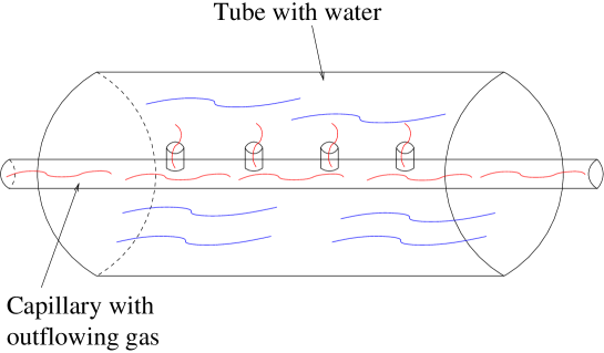
Figure 1: Sketch of the real-life experiment (capillary with gaseous outflow into a tube filled with water).

We consider the profile of the tube and deal with the simplified approach of the experiment, which is given in Figure 2.

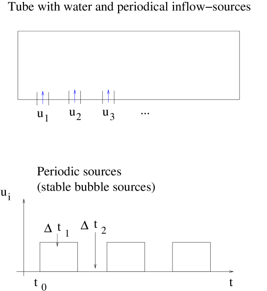
Figure 2: Periodically inflow of the stable bubble sources.

Based on the decoupling of formation and transport, while we assume, that the formation process is not influenced by the transport, see [2], we deal with two different decoupled models:

• Near-field approach based on a Young-Laplace equation, see [15], where we have a static shape after the formation of the bubbles.

• Far-field approach based on a convection-diffusion equation, see [4], where we have a rewriting into a level-set equation, such that we could transport the static bubble-shapes, see [12].

In the following, we discuss the different models.

2.1 Far-field approach

The first modelling approach is given with a convection-diffusion equation in cylindrical coordinate as:

$$\frac{\partial u}{\partial t}=-v\frac{\partial u}{\partial z}+D_{L}\frac{\partial^{2}u}{\partial z^{2}}+\frac{D_{t}}{r}\frac{\partial}{\partial r}(r\frac{\partial u}{\partial r}),\;(r,z,t)\in\Omega\times[0,T],$$ (1)

$$u(x,z,0)=u_{near}(x,z),\;(r,z,t)\in\Omega,$$ (2)

where we assume $u_{near}$ is the solution of the bubble-formation in the near-field and we assume to have Dirichlet-boundary conditions.

Here, we have the benefit and drawbacks of the modelling approach:

• Benefits:

  • The model is simple and fast to compute.

  • The model also allows to discuss a dynamical shape.

• Drawbacks:

  • The shape of the bubble is not preserved, while we assume a static shape.

  • The influence of the speed of motion in the outer normal direction is not possible.

2.2 Level-Set method

We apply an improved model, that allows to follow the shapes of the bubble, see [12].

The convection-diffusion equation is reformulated in the notation of a level-set equation, which is given as

$$\frac{\partial u}{\partial t}=-{\bf v}\cdot\nabla u-F_{0}|\nabla u|,\;({\bf x},t)\in\Omega\times[0,T],$$ (3)

$$u({\bf x},0)=u_{0}({\bf x}),$$ (4)

$$u(0,t)=u(2,t)=0.0,\;({\bf x},t)\in\partial\Omega\times[0,T],$$ (5)

where ${\bf v}$ is the convection vector and $F_{0}$ is the speed of motion in the outer normal direction. Further $\Omega$ is the computational domain and $T$ is the end time. The initialisation $u({\bf x},0)$ is the results of the near-field computations.

Such equations are wel-known as level-set equations and can be solved like convection-diffusion equations, see [12].

In the following, we apply the explicit different discretization methods in space, while we apply the level-set equation with the explicit time-discretisation and apply upwind methods for the advection and outer normal direction term only in the $x$-direction, the same is also done with the $y$-direction.

We have the following terms:

$$D^{-}_{x}u_{i,j}=\frac{u_{i,j}-u_{i-1,j}}{\Delta x},$$ (6)

$$D^{+}_{x}u_{i,j}=\frac{u_{i+1,j}-u_{i,j}}{\Delta x},$$ (7)

$$|D^{+}_{x}u_{i,j}|=\left((\max(D^{-}_{x}u_{i,j},0))^{2}+(\min(D^{+}_{x}u_{i,j},0))^{2}\right)^{1/2},$$ (8)

$$u_{i}^{n+1} =u_{i}^{n}-\Delta t\;v_{x}\frac{u_{i}^{n}-u_{i-1}^{n}}{\Delta x}-\Delta t\;v_{y}\frac{u_{i,j}^{n}-u_{i,j-1}^{n}}{\Delta x}$$

$$+\Delta t\;F_{o}|D^{+}_{x}u_{i,j}|,$$ (9)

where we assume $v_{x},v_{y},F_{0}\geq 0$.

We discretize the Level-set equation with the explicit time-discretisation and apply upwind methods for the advection and outer normal direction term in the $x$- and $y$-direction and have the following terms:

$$D^{-}_{x}u_{i,j}=\frac{u_{i,j}-u_{i-1,j}}{\Delta x},$$ (10)

$$D^{+}_{x}u_{i,j}=\frac{u_{i+1,j}-u_{i,j}}{\Delta x},$$ (11)

$$D^{-}_{y}u_{i,j}=\frac{u_{i,j}-u_{i,j-1}}{\Delta y},$$ (12)

$$D^{+}_{y}u_{i,j}=\frac{u_{i,j+1}-u_{i,j}}{\Delta y},$$ (13)

$$|D^{+}_{x}u_{i,j}|=\left((\max(D^{-}_{x}u_{i,j},0))^{2}+(\min(D^{+}_{x}u_{i,j},0))^{2}\right.$$ (14)

$$\left.+(\max(D^{-}_{y}u_{i,j},0))^{2}+(\min(D^{+}_{y}u_{i,j},0))^{2}\right)^{1/2}.$$ (15)

$$u_{i}^{n+1} =u_{i}^{n}-\Delta t\;v_{x}\frac{u_{i}^{n}-u_{i-1}^{n}}{\Delta x}-\Delta t\;v_{y}\frac{u_{i,j}^{n}-u_{i,j-1}^{n}}{\Delta x}$$

$$+\Delta t\;F_{o}|D^{+}_{x}u_{i,j}|,$$ (16)

where we assume $v_{x},v_{y},F_{0}\geq 0$.

Remark 1

An alternative approach of the shape transport can be done with the volume of fluid (VOF) method. Such a method is based on a free-surface modelling technique, while the method is tracking and locating the free surface, see also [7].

In the following, we discuss the near-field approach.

2.3 Near field model

The near-field model is discussed with respect to the formation of a drop or bubble, see [15] and [13].

The basic modelling idea is based on the so called Young-Laplace equation, see [3] and deals with the following simplied shape of the bubble, see Figure 3.

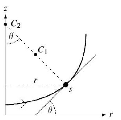
Figure 3: Near field parameters of the bubble shape.

We deal with the following parameterisation, see [15]:

$$\beta=-\rho gR_{t}^{2}/\sigma,$$ (17)

where $\beta$ is the Bond number, $\sigma$ is the surface tension, $\rho$ is the liquid density, $g$ is the gravity and $R_{t}$ is the curvature of the drop.

The near-field equations are given as:

$$\frac{dr}{ds}=\cos(\theta),$$ (20)

$$\frac{dz}{ds}=\sin(\theta),$$

$$\frac{d\theta}{ds}=2+\beta z-\frac{\sin(\theta)}{r},$$

where $s$ is the arc length along the curve and $\theta$ the angle of elevation for its slope and $\alpha$ is the mono-layer surface tension.

We have the conditions:

$$r=a,\;z=0,\;\mbox{at}\;s=0,$$ (21)

$$r=0,\;\frac{dz}{ds}=\frac{dz}{dr}=0,\;\mbox{at}\;s=L,$$ (22)

where $L$ is the arc length of the bubble which is a-priori unknown and is numerically computed via the boundary value problem. Further, we apply $r=a\rightarrow 0$.

Remark 2

The ODE system based on a boundary value problem can be solved with numerical methods, e.g., with the MATLAB function bvp4c. Based on the boundary values, we solve the possible curvature of the bubble. We assume an axial-symmetric bubble and solve the half shape, then we measure the different diameters of the bubble-ellipse.

3 Near-Field Solver: System of ordinary differential equations with boundary conditions

For the near-field, we have to solve a BVP for ODEs, see [11] and [10].

We assume the following nonlinear ODE, give as:

$$\frac{dy}{dt}=A(t)y+q(t),\;t\in[a,b],$$ (23)

$$B_{a}y(a)+B_{b}y(b)=d,$$ (24)

where ${\bf y},{\bf q}(t),d\in{\rm I}\!{\rm R}^{n}$ and $A(t),B_{a},B_{b}\in{\rm I}\!{\rm R}^{n\times}$, see [10].

Then, we have the following multiple shooting algorithm, given as

Algorithm 3.1

We have a mesh $a=t_{1}<t_{2}<\ldots<t_{N+l}=b$, on each mesh interval $[t_{i},t_{i+1}]$ with $1\leq i\leq N$, we solve

1. A fundamental solution

   $$Y_{i}^{\prime}=A(t)Y_{i},\;Y_{i}(t_{i})=F_{i},$$ (25)

2. A particular solution

   $${\bf v}_{i}^{\prime}=A(t){\bf v}_{i}+{\bf q}(t),\;{\bf v}_{i}(t_{i})={\bf e}_{i},$$ (26)

3. Then, we find the vector ${\bf s}_{i}\in{\rm I}\!{\rm R}^{n}$, $1\leq i\leq N$:

   $${\bf y}_{i}^{\prime}=Y_{i}(t){\bf s}_{i}+{\bf v}_{i}(t),\;{\bf v}_{i}(t_{i})={\bf e}_{i},$$ (27)

Remark 3

The algorithm 3.1 allows to compute the boundary value problem also with respect to the Neumann-boundary conditions. Based on the iterative scheme, we also solve the nonlinearity of the equation-system.

4 Coupling Near-Field and Far-Field

The modelling assumes, that we could decouple the near and far-field, while we neglect the coalescence or ruptures of the bubbles, e.g., in the flow-field, see [9].

We assume that in terms of the bubble-density function:

$$f_{b}(r,z,x,y,t)=u(x,y,t)\delta((r-R(x,y,t)),(z-Z(x,y,t))),$$ (28)

where $u$ is the concentration of the bubble and $R$ and $Z$ are obtained with the bubble-formation equations, while $r$ and $z$ are the cylinder coordinates of the density function, that we do not have an influence means $r\approx R$ and $z\approx Z$ for the formation process.

We discuss the following different coupling ideas:

• Parameters of the ellipse are computed in the near-field and initialise the far-field bubble.

• The near-field computation is directly implemented into the far-field.

4.1 Decoupled computation of Near- and Far-Field

The near-field bubble is computed with the ODE’s given in (20)-(20).

We estimate the characteristic parameters of the ellipse in the Figure 4.

Figure 4: Final bubble based on the near-field computation and estimation of the bubble-parameters (we assume an elliptic curve).

Based on the estimation of the elliptic-parameters, we obtain the curvature of the ellipse:

$$\frac{(x-x_{a})^{2}}{a^{2}}+\frac{(y-y_{b})^{2}}{b^{2}}=1.$$ (29)

The ellipse is the curvature of the far-field, which is computed with the level-set method.

Remark 4

The transformation of the elliptic parameters of the near-field model allows to simplify the construction of the shape in the far-field. We only apply the ellipses in the far-field transport modell.

4.2 Coupled computation of Near- and Far-Field

Based on the electric-field on smaller time-scale, we have to update the near-field and far-field coupling in a numerical cycle,

The near-field bubble is computed with the ODE’s and with the underlying influence of the E-field. Further the far-field is computed by the transport equation with level-set methods. We couple the coupling via an interpolation between the mesh-free space of the near-field and the grid-space of the far-field with the give diameters of the bubbles and the trajectories of the transport field

The oscillation of the spherical bubble, see [9], [14] and [1], is given as:

$$r=r_{0}+r_{\epsilon},$$ (30)

$$r_{\epsilon}=-r_{\epsilon_{0}}\exp(i\;\omega_{0}t),$$ (31)

where $r_{0}$ is the mean radius, $\omega_{0}$ is the resonance frequency and $r_{\epsilon_{0}}$ amplitude of maximal oscillations of the bubble radius.

The characteristic frequency of the breathing mode with respect to the electric stress (pressure) is given as:

$$\omega_{0}=\frac{1}{2\pi r_{0}}\sqrt{\frac{3\;k\;p}{\rho}-\frac{2\sigma}{\rho\;r_{0}}},$$ (32)

where $\sigma$ is the gas-liquid surface tension, $\rho$ is the liquid density, $k$ is the polytropic exponent ($k=1.4$ for air). $p$ is the pressure, where $p=|p_{0}-p_{E}|$ with $p_{0}$ is the hydrostatic pressure in the fluid far from the bubble and $p_{E}$ is the electric stress (pressure) given of the electric field with

$$p_{E}=\frac{9}{8}\epsilon|{\bf E}_{0}|^{2}\;\sin^{2},$$ (33)

the pressure maximum is given at $\theta=\pi/2$, $\epsilon$ is the peremitivity and ${\bf E}_{0}$ is the uniform electric field.

The numerical cycle is given in Figure 5.

Figure 5: Numerical cycle of the near-far-field coupling.

In the following, we discuss the detailed coupling of the near-field and far-field, see Figure 6.

Figure 6: Near field and far field coupling in the E-field.

Remark 5

The accuracy of the cycle is give with respect to the step-size of the far-field.

5 Numerical Experiments

In the following, we apply the different numerical experiments based on the bubble-formation and the bubble-transport. While the bubble-formation is based on the model with Young-Laplace equation, the bubble-transport model is based on the level-set equations.

5.1 Bubble-Formation: Experiment 1

The near-field equations are given as:

$$\frac{dr}{ds}=\cos(\theta),$$ (34)

$$\frac{dz}{ds}=\sin(\theta),$$ (35)

$$\frac{d\theta}{ds}=-\frac{\sin(\theta)}{r}+\frac{\Delta p}{\alpha},$$ (36)

or in vectorial form:

$$\frac{dy}{dt}=\tilde{A}(y(t))+\tilde{q}(t),\;t\in[t_{i},t_{i+1}],$$ (37)

where $\tilde{A}(y(t))=\left(\begin{array}[]{c}\cos(\theta)\\ \sin(\theta)\\ -\frac{\sin(\theta)}{r}\end{array}\right)$ and $\tilde{q}(t)=\left(\begin{array}[]{c}0\\ 0\\ \frac{\Delta p}{\alpha}\end{array}\right)$. Further, $y(t)=(r(t),z(t),\theta(t))^{t}$ and $t$ is the arc length along the curve and $r$ is the radius, $z$ is the vertical distance and $\theta$ the angle of elevation for its slope and $\alpha$ is the mono-layer surface tension.

We have to linearise the equations, which are given as:

$$\frac{dy}{dt}=\tilde{A}(y(t_{i}))+\frac{\partial\tilde{A}}{\partial y}|_{y(t_{i})}(y(t)-y(t_{i}))+\tilde{q}(t),\;t\in[t_{i},t_{i+1}],$$ (38)

$$\frac{dy}{dt}=A(t)y(t)+q(t),\;t\in[t_{i},t_{i+1}],$$ (39)

$$B_{a}y(a)+B_{b}y(b)=d,$$ (40)

where $A(t)=\frac{\partial\tilde{A}}{\partial y}|_{y(t_{i})}y(t)$, $q(t)=\tilde{A}(y(t_{i}))-\frac{\partial\tilde{A}}{\partial y}|_{y(t_{i})}y(t_{i})+\tilde{q}(t)$. Further, we have $y=(r,z,\theta)^{t}$ and

$$\frac{\partial A}{\partial y}|_{y(t_{i})}=\left(\begin{array}[]{ccc}0&0&-\sin(\theta(t_{i}))\\ 0&0&\cos(\theta(t_{i}))\\ -\frac{\sin(\theta(t_{i}))}{r^{2}(t_{i})}&0&-\frac{\cos(\theta(t_{i}))}{r(t_{i})}\end{array}\right).$$ (44)

We have the conditions:

$$r=a,\;z=0,\;\theta=\pi/2,\;\mbox{at}\;t=0,$$ (45)

$$r=0,\;\frac{dz}{ds}=0,\;\theta=2(\pi/2),\mbox{at}\;t=L,$$ (46)

where $a$ is the radius of the bubble, $L$ is the arc length of the bubble which is a-priori unknown, where we start with $L=L_{0}=\frac{2\pi a^{2}}{4}$ and we go on with $L=L_{1}\leq L_{2}\leq\ldots\leq L_{stop}$.

We have the following linear equation system:

$$\left[\begin{array}[]{llllll}S_{1}&R_{1}&\\ &S_{2}&R_{2}&\\ &&\ddots&\ddots&\\ &&&S_{N}&R_{N}\\ B_{a}&&&B_{b-1}&B_{b}\end{array}\right]\left[\begin{array}[]{l}y_{1}\\ y_{2}\\ \vdots\\ y_{N}\\ y_{N+1}\end{array}\right]=\left[\begin{array}[]{l}q_{1}\\ q_{2}\\ \vdots\\ q_{N}\\ d\end{array}\right]$$ (62)

4 where $S_{i}=R_{i}=-h_{i}^{-1}I-\frac{1}{2}A(t_{i+1/2})$, $q_{i}=q(t_{i+1/2}$ with $h_{i}=t_{i+1}-t_{i}$, $t_{i+1/2}=t_{i}+\frac{1}{2}h_{i}$.

Further, we have the matrices and vectors:

$$B_{a}=\left(\begin{array}[]{ccc}0&0&0\\ 0&0&0\\ 0&0&0\end{array}\right),$$ (66)

$$B_{b-1}=\left(\begin{array}[]{ccc}0&0&0\\ 0&1&0\\ 0&0&0\end{array}\right),$$ (70)

$$B_{b}=\left(\begin{array}[]{ccc}1&0&0\\ 0&1&0\\ 0&0&1\end{array}\right),$$ (74)

$$d=\left(\begin{array}[]{ccc}L\\ 0\\ 0\end{array}\right).$$ (78)

• Test example 1:
  We apply the following test-example with the a quarter of a circle, means $L=2\pi a^{2}/4$, where $a=1,2,3,3.5$ and we assume $N=L/\Delta t$, where we assume $\Delta t=2\pi\;0.001$ and $\frac{\Delta p}{\alpha}=0$.

• Test example 2:
  We have $N=L/\Delta t$, where we assume $\Delta t=0.001$ and $L=2$ and $\frac{\Delta p}{\alpha}=0,0.8,1.4$.

The numerical results of bubble-formation is given in Figure 7.

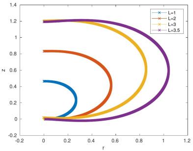
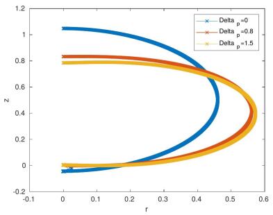
Figure 7: Bubble-formation, left figure with different length $L$ and $\frac{\Delta p}{\alpha}=0$, while $L=2$ is exact solution of the $1/4$ circle and right figure with different right-hand side-parameters $\frac{\Delta p}{\alpha}$ and for $L=2$.

Remark 6

The Young-Laplace equation allows to formulate the bubble-formation such that we could obtain the radii of the different bubbles based on the various pressure parameters. We also compare the results with respect to the computations in the Literature, see [13].

5.2 Bubble-Formation: Experiment 2

In the following, we couple the near-field and far-field computations.

We have the following setting, see Figure 8.

Figure 8: Left figure: Bubble-formation with the ODEs and right figure: Bubble-transport with the PDEs (level-set equations).

We apply the following parameters:

• Input-parameters of the near-field bubbles:

  • $r_{1}(0)=0.01,\;z_{1}(0)=0,\;r_{1}(L)=0,\;L=1,\;\frac{\Delta p_{1}}{\alpha_{1}}=0.8$,

  • $r_{2}(0)=0.01,\;z_{2}(0)=0,\;r_{2}(L)=0,\;L=2,\;\frac{\Delta p_{2}}{\alpha_{2}}=0.8$.

• We compute the bubbles based on the near-field code and obtain the ellipse-diameters $a_{bubble},\;b_{bubble}$.

• We initialise the two ellipses for the far-field computations given as:

  • $(x-20)^{2}+((y-100)*a_{bubble,1}/b_{bubble,1})^{2}-a_{bubble,1}^{2}$,

  • $(x-70)^{2}+((y-90)*a_{bubble,2}/b_{bubble,2})^{2}-a_{bubble,2}^{2}$.

The numerical results of near-field bubble-formation is given in Figure 9.

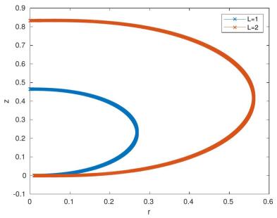
Figure 9: The computation of the bubble formation (near-field) for two bubbles.

The numerical results of the near-far-field coupled bubble-transport code, which is given in Figure 10.

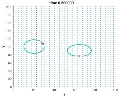
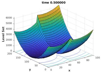
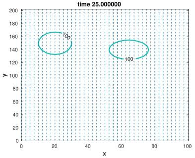
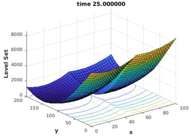
Figure 10: Upper figures: Transport of the two bubble with the level-set function at time $t=0.1$, lower figures: Transport of the two bubble with the level-set function at time $t=25$.

Remark 7

The coupling of the formation and transport of the bubbles are done with ordinary and partial differential equations. Based on decoupling such systems of mixed ordinary and partial differential equations, we could compute each separate part with the optimal numerical solvers.

5.3 Bubble-Formation: Multiple Bubble Experiment (10 Bubbles)

In the following, we extend the near-field and far-field computations with 10 bubbles. We also apply the decomposition of near-field and far-field computations as given in Figure 8.

We apply the following parameters:

• Computation of the near-field bubbles (a representing bubble is computed)

  • Input-parameters of the near-field bubbles computation:

    • Bubble 1:
      $r_{1}(0)=0.01,\;z_{1}(0)=0,\;r_{1}(L)=0,\;L=2,\;\frac{\Delta p_{1}}{\alpha_{1}}=0.2$,

    • Bubble 2:
      $r_{2}(0)=0.01,\;z_{2}(0)=0,\;r_{2}(L)=0,\;L=2,\;\frac{\Delta p_{2}}{\alpha_{2}}=0.4$.

    • Bubble 3:
      $r_{3}(0)=0.01,\;z_{3}(0)=0,\;r_{3}(L)=0,\;L=2,\;\frac{\Delta p_{3}}{\alpha_{3}}=0.6$.

    • Bubble 4:
      $r_{4}(0)=0.01,\;z_{4}(0)=0,\;r_{4}(L)=0,\;L=2,\;\frac{\Delta p_{4}}{\alpha_{4}}=0.8$.

    • Bubble 5:
      $r_{5}(0)=0.01,\;z_{5}(0)=0,\;r_{5}(L)=0,\;L=2,\;\frac{\Delta p_{5}}{\alpha_{5}}=1.0$.

    • Bubble 6:
      $r_{6}(0)=0.01,\;z_{6}(0)=0,\;r_{6}(L)=0,\;L=2,\;\frac{\Delta p_{6}}{\alpha_{6}}=1.2$.

    • Bubble 7:
      $r_{7}(0)=0.01,\;z_{7}(0)=0,\;r_{7}(L)=0,\;L=2,\;\frac{\Delta p_{7}}{\alpha_{7}}=1.4$.

    • Bubble 8:
      $r_{8}(0)=0.01,\;z_{8}(0)=0,\;r_{8}(L)=0,\;L=2,\;\frac{\Delta p_{8}}{\alpha_{8}}=1.6$.

    • Bubble 9:
      $r_{9}(0)=0.01,\;z_{9}(0)=0,\;r_{9}(L)=0,\;L=2,\;\frac{\Delta p_{9}}{\alpha_{9}}=1.8$.

    • Bubble 10:
      $r_{10}(0)=0.01,\;z_{10}(0)=0,\;r_{10}(L)=0,\;L=2,\;\frac{\Delta p_{10}}{\alpha_{10}}=2.0$.

  • Output-parameters of the near-field bubble computation:

    • Bubble 1:
      $a_{bubble_{1}}=0.5141,\;b_{bubble_{1}}=0.9926$.

    • Bubble 2:
      $a_{bubble_{2}}=0.5219,\;b_{bubble_{2}}=0.9718$.

    • Bubble 3:
      $a_{bubble_{3}}=0.5295,\;b_{bubble_{3}}=0.9506$.

    • Bubble 4:
      $a_{bubble_{4}}=0.5369,\;b_{bubble_{4}}=0.9289$.

    • Bubble 5:
      $a_{bubble_{5}}=0.5443,\;b_{bubble_{5}}=0.9067$.

    • Bubble 6:
      $a_{bubble_{6}}=0.5514,\;b_{bubble_{6}}=0.8841$.

    • Bubble 7:
      $a_{bubble_{7}}=0.5584,\;b_{bubble_{7}}=0.8612$.

    • Bubble 8:
      $a_{bubble_{8}}=0.5651,\;b_{bubble_{8}}=0.8382$.

    • Bubble 9:
      $a_{bubble_{9}}=0.5717,\;b_{bubble_{9}}=0.8154$.

    • Bubble 10:
      $a_{bubble_{10}}=0.5780,\;b_{bubble_{10}}=0.7928$.

  • Ellipse: $(x-x_{bubble_{i}})^{2}+((y-y_{bubble_{i}})*a_{bubble}/b_{bubble})^{2}-a_{bubble}^{2}$,
    where $(x_{bubble_{i}},y_{bubble_{i}})$ is the origin of the $i$-th bubble.

• Computation of the far-field bubbles (level-set initialisation):

  • Parameterisation of the level-set initial-function, e.g., two bubbles:

    $$\phi_{0}(x,y)=\left\{\begin{array}[]{cc}(x-x_{bubble_{1}})^{2}+((y-y_{bubble_{1}})\frac{a_{bubble_{1}}}{b_{bubble_{1}}})^{2}-a_{bubble_{1}}^{2},&\\ a_{x}\leq x\leq 50,\;a_{y}\leq x\leq b_{y},&\\ (x-x_{bubble_{2}})^{2}+((y-y_{bubble_{2}})\frac{a_{bubble_{2}}}{b_{bubble_{2}}})^{2}-a_{bubble_{2}}^{2},&\\ 50\leq x\leq b_{x},\;a_{y}\leq x\leq b_{y},&\\ \end{array}\right.$$ (83)

    where $(x_{bubble_{1}},y_{bubble_{1}})=(20,50)$, $(x_{bubble_{2}},y_{bubble_{2}})=(80,50)$ with the coordinates of the grid $(a_{x},a_{y})=(0,0)$ and $b_{x},b_{y})=(100,200)$.

The numerical results of the formation of the bubbles are given in Figures 11.

Figure 11: Formation of 10 bubbles with the different pressure-terms.

The numerical results of the near-far-field coupled bubble-transport code, which is given in Figures 12 and 13.

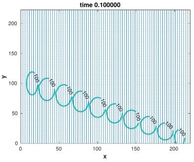
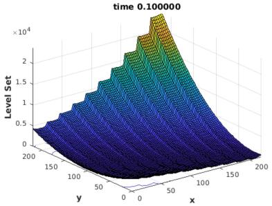
Figure 12: Transport of 10 bubbles with the level-set function at the initialisation $t=0.1$.

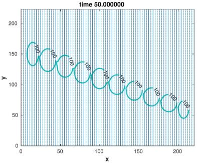
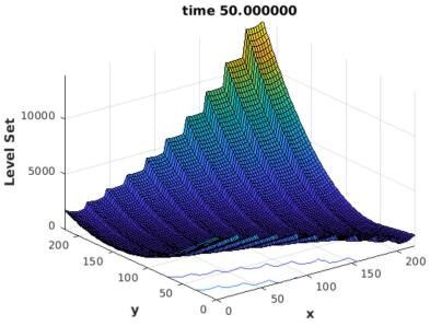
Figure 13: Transport of 10 bubbles with the level-set function at time $t=50$.

Remark 8

In the experiment, we deal with at least 10 bubbles, which are different formated and transported via the level-set method. The numerical experiments allows to accelerate the formation and transport of such processes.

5.4 Bubble-Formation: Oscillation of the Air-Bubbles in the electrical-Field (first modelling approach)

In the following, we simulate a bubble filled with air in a electrical field, see [14].

We have the following setting of the influenced bubble, see Figure 14.

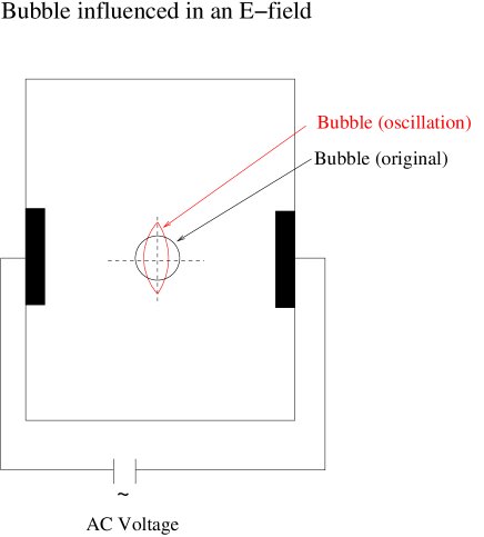
Figure 14: Bubble-formation influenced by an electrical field.

We apply the following near-field equation based on an extension of the pressure-term with an E-field.

The near-field equations are given as:

$$\frac{dr}{ds}=\cos(\theta),$$ (84)

$$\frac{dz}{ds}=\sin(\theta),$$ (85)

$$\frac{d\theta}{ds}+\frac{\sin(\theta)}{r}=\frac{\Delta p}{\alpha},$$ (86)

where $s$ is the arc length along the curve and $\theta$ the angle of elevation for its slope and $\alpha$ is the mono-layer surface tension.

Further, we have

$$\Delta p=p_{bubble}-p_{tube}=\rho gz-p_{tube},$$ (87)

where $p_{tube}=p_{E}=\frac{9}{8}|{\bf E}_{0}|^{2}\;\sin(\theta)$ is the pressure based on the electrical field of the tube and we obtain:

$$\frac{dr}{ds}=\cos(\theta),$$ (88)

$$\frac{dz}{ds}=\sin(\theta),$$ (89)

$$\frac{d\theta}{ds}+\frac{\sin(\theta)}{r}=\frac{\rho gz-\frac{9}{8}|{\bf E}_{0}|^{2}\;\sin(\theta)}{\alpha}.$$ (90)

We apply the following parameters:

• Computation of the near-field bubbles (a representing bubble is computed)

  • Input-parameters of the near-field bubbles computation:

    • Bubble 1:
      $r_{1}(0)=0.01,\;z_{1}(0)=0,\;r_{1}(L)=0,\;L=2,\;\frac{\Delta p_{1}}{\alpha_{1}}=0.2$,

    • Bubble 2:
      $r_{2}(0)=0.01,\;z_{2}(0)=0,\;r_{2}(L)=0,\;L=2,\;\frac{\Delta p_{2}}{\alpha_{2}}=0.4$.

    • Bubble 3:
      $r_{3}(0)=0.01,\;z_{3}(0)=0,\;r_{3}(L)=0,\;L=2,\;\frac{\Delta p_{3}}{\alpha_{3}}=0.6$.

    • Bubble 4:
      $r_{4}(0)=0.01,\;z_{4}(0)=0,\;r_{4}(L)=0,\;L=2,\;\frac{\Delta p_{4}}{\alpha_{4}}=0.8$.

    • Bubble 5:
      $r_{5}(0)=0.01,\;z_{5}(0)=0,\;r_{5}(L)=0,\;L=2,\;\frac{\Delta p_{5}}{\alpha_{5}}=1.0$.

    • Bubble 6:
      $r_{6}(0)=0.01,\;z_{6}(0)=0,\;r_{6}(L)=0,\;L=2,\;\frac{\Delta p_{6}}{\alpha_{6}}=1.2$.

    • Bubble 7:
      $r_{7}(0)=0.01,\;z_{7}(0)=0,\;r_{7}(L)=0,\;L=2,\;\frac{\Delta p_{7}}{\alpha_{7}}=1.4$.

    • Bubble 8:
      $r_{8}(0)=0.01,\;z_{8}(0)=0,\;r_{8}(L)=0,\;L=2,\;\frac{\Delta p_{8}}{\alpha_{8}}=1.6$.

    • Bubble 9:
      $r_{9}(0)=0.01,\;z_{9}(0)=0,\;r_{9}(L)=0,\;L=2,\;\frac{\Delta p_{9}}{\alpha_{9}}=1.8$.

    • Bubble 10:
      $r_{10}(0)=0.01,\;z_{10}(0)=0,\;r_{10}(L)=0,\;L=2,\;\frac{\Delta p_{10}}{\alpha_{10}}=2.0$.

  • Electrical field parameters are given as:

    $\alpha=0.1$, $\rho=0.1,\;g=9.81,\;|{\bf E}_{0}|^{2}=0.1$.

  • Output-parameters of the near-field bubble computation (formation):

    • Bubble 1:
      $a_{bubble_{1}}=0.5141,\;b_{bubble_{1}}=0.9926$.

    • Bubble 2:
      $a_{bubble_{2}}=0.5219,\;b_{bubble_{2}}=0.9718$.

    • Bubble 3:
      $a_{bubble_{3}}=0.5295,\;b_{bubble_{3}}=0.9506$.

    • Bubble 4:
      $a_{bubble_{4}}=0.5369,\;b_{bubble_{4}}=0.9289$.

    • Bubble 5:
      $a_{bubble_{5}}=0.5443,\;b_{bubble_{5}}=0.9067$.

    • Bubble 6:
      $a_{bubble_{6}}=0.5514,\;b_{bubble_{6}}=0.8841$.

    • Bubble 7:
      $a_{bubble_{7}}=0.5584,\;b_{bubble_{7}}=0.8612$.

    • Bubble 8:
      $a_{bubble_{8}}=0.5651,\;b_{bubble_{8}}=0.8382$.

    • Bubble 9:
      $a_{bubble_{9}}=0.5717,\;b_{bubble_{9}}=0.8154$.

    • Bubble 10:
      $a_{bubble_{10}}=0.5780,\;b_{bubble_{10}}=0.7928$.

  • Output-parameters of the near-field bubble computation (in the E-field):

    • Bubble 1:
      $a_{bubble_{1}}=0.5558,\;b_{bubble_{1}}=0.8698$.

    • Bubble 2:
      $a_{bubble_{2}}=0.5626,\;b_{bubble_{2}}=0.8468$.

    • Bubble 3:
      $a_{bubble_{3}}=0.5693,\;b_{bubble_{3}}=0.8239$.

    • Bubble 4:
      $a_{bubble_{4}}=0.5757,\;b_{bubble_{4}}=0.8013$.

    • Bubble 5:
      $a_{bubble_{5}}=0.5819,\;b_{bubble_{5}}=0.7789$.

    • Bubble 6:
      $a_{bubble_{6}}=0.5878,\;b_{bubble_{6}}=0.7571$.

    • Bubble 7:
      $a_{bubble_{7}}=0.5935,\;b_{bubble_{7}}=0.7359$.

    • Bubble 8:
      $a_{bubble_{8}}=0.5990,\;b_{bubble_{8}}=0.7153$.

    • Bubble 9:
      $a_{bubble_{9}}=0.6042,\;b_{bubble_{9}}=0.6953$.

    • Bubble 10:
      $a_{bubble_{10}}=0.6091,\;b_{bubble_{10}}=0.6760$.

  • Ellipse: $(x-x_{bubble_{i}})^{2}+((y-y_{bubble_{i}})*a_{bubble}/b_{bubble})^{2}-a_{bubble}^{2}$,
    where $(x_{bubble_{i}},y_{bubble_{i}})$ is the origin of the $i$-th bubble.

• Computation of the far-field bubbles (level-set initialisation):

  • Parameterisation of the level-set initial-function, e.g., two bubbles:

    $$\phi_{0}(x,y)=\left\{\begin{array}[]{cc}(x-x_{bubble_{1}})^{2}+((y-y_{bubble_{1}})\frac{a_{bubble_{1}}}{b_{bubble_{1}}})^{2}-a_{bubble_{1}}^{2},&\\ a_{x}\leq x\leq 50,\;a_{y}\leq x\leq b_{y},&\\ (x-x_{bubble_{2}})^{2}+((y-y_{bubble_{2}})\frac{a_{bubble_{2}}}{b_{bubble_{2}}})^{2}-a_{bubble_{2}}^{2},&\\ 50\leq x\leq b_{x},\;a_{y}\leq x\leq b_{y},&\\ \end{array}\right.$$ (95)

    where $(x_{bubble_{1}},y_{bubble_{1}})=(20,50)$, $(x_{bubble_{2}},y_{bubble_{2}})=(80,50)$ with the coordinates of the grid $(a_{x},a_{y})=(0,0)$ and $b_{x},b_{y})=(100,200)$.

The numerical results of the formation of the bubbles with and without the E-field are given in Figures 15.

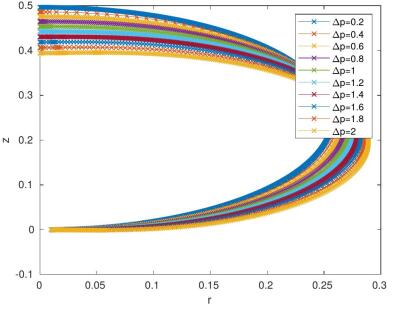
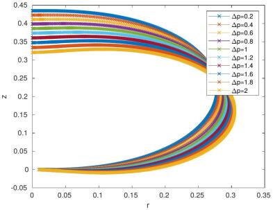
Figure 15: Left figure: Formation of 10 bubbles without an E-field, right figure: Formation of 10 bubbles with an E-field.

The numerical results of the near-far-field coupled bubble-transport code, which is given in Figures 16 and 17.

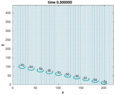
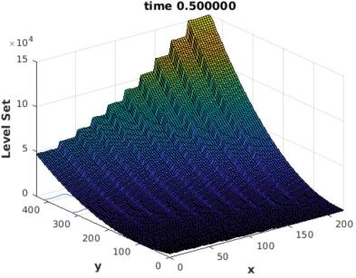
Figure 16: Transport of 10 bubbles in the E-field with the level-set function at the initialisation $t=0.1$.

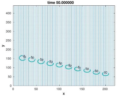
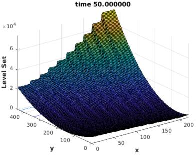
Figure 17: Transport of 10 bubbles in the E-field with the level-set function at time $t=50$.

Remark 9

The bubble modifications are given by the E-field, while it changes the formation of the bubble. The level-set method is modified by multi-level-set domains and allows to deal with different level-set functions, such that we could transport multiple bubbles with E-fields. In the first approach, we assume, that the E-field can be approximated at the beginning of the formation and that the bubble will not be changed after such a initial formation.

6 Conclusion

We present a bubble model, which is a coupled model based on a bubble formation and bubble transport model. The decoupling into near- and far-field models allows to apply optimal solver and discretization methods. We apply different numerical experiments, which shows the benefit of such a treatment. In future, we consider the fully coupled problem, while we deal with bubble density functions and the coupling between the formation and transport process. Such an extension allows to see the ruptures of the bubbles.

References

• [1] T. Bellini, M. Corti, A. Gelmetti and P. Lago. Interferometric study of selectively excited bubble capillary modes. Europhysics Letters, 38(7):521-526, 1997.
• [2] C.E. Brennen. Cavitation and Bubble Dynamics. Oxford University Press, New York, Oxford, 1995.
• [3] R. Finn. Equilibrium Capillary Surfaces. Springer-Verlag New York, 1986.
• [4] J. Geiser. Multicomponent and Multiscale Systems: Theory, Methods, and Applications in Engineering. Springer, Cham, Heidelberg, New York, Dordrecht, London, 2016.
• [5] H. Gu *, M.H.G. Duits and F. Mugele. Droplets Formation and Merging in Two-Phase Flow Microfluidics. Int. J. Mol. Sci., 12:2572-2597, 2011.
• [6] T. Hayashi, S. Uehara, H. Takana and H. Nishiyama. Gas-liquid two-phase chemical reaction model of reactive plasma inside a bubble for water treatment. Proceeding of the 22nd International Symposium on Plasma Chemistry July 5-10, Antwerp, Belgium, 2015.
• [7] C.W. Hirt and B.D. Nichols. Volume of fluid (VOF) method for the dynamics of free boundaries. Journal of Computational Physics, 39 (1):201-225, 1981.
• [8] R. Kumar and N.R. Kuloor. The formation of bubbles and drops. Advances in Chemical Engineering, 8:255-368, 1970.
• [9] T.G. Leighton. The Acoustic Bubble. Academic press, London, San Diego, 1994.
• [10] L. Liu and R.D. Russell. Linear system solver for boundary value ODEs. Journal of Computational and Applied Mathematics, 45: 103-117, 1993.
• [11] M.R. Osborne. On Shooting Methods for Boundary Value Problems. Journal of Mathematical Analysis and Application, 27: 417-433, 1969.
• [12] J.A. Sethian. Level Set Methods: Evolving Interfaces in Geometry, Fluid Mechanics, Computer Vision, and Materials Science. Cambridge University Press 1996
• [13] J.A. Simmons and J.E. Sprittles and Y.D. Shikhmurzaev. The formation of a bubble from a submerged orifice. European Journal of Mechanics - B/Fluids, 53, Supplement C, 24-36, 2015.
• [14] B.S. Sommers and J.E. Foster. Nonlinear oscillations of gas bubbles submerged in water: implications for plasma breakdown. Journal of Physics D: Applied Physics 45(41): 415203, 2012.
• [15] S.T. Thoroddsen, K. Takehara, and T.G. Etoh. The coalescence speed of a pendent and a sessile drop. Journal of Fluid Mechanics, Cambridge University Press, 527: 85-114, 2005.
• [16] G.Q. Yang, B. Du, and L.S. Fan. Bubble formation and dynamics in gas–liquid–solid fluidization - A review. Chemical Engineering Science 62, 2-27, 2007.