Modeling Surface Appearance from a Single Photograph using Self-augmented Convolutional Neural Networks

Abstract.

We present a convolutional neural network (CNN) based solution for modeling physically plausible spatially varying surface reflectance functions (SVBRDF) from a single photograph of a planar material sample under unknown natural illumination. Gathering a sufficiently large set of labeled training pairs consisting of photographs of SVBRDF samples and corresponding reflectance parameters, is a difficult and arduous process. To reduce the amount of required labeled training data, we propose to leverage the appearance information embedded in unlabeled images of spatially varying materials to self-augment the training process. Starting from an initial approximative network obtained from a small set of labeled training pairs, we estimate provisional model parameters for each unlabeled training exemplar. Given this provisional reflectance estimate, we then synthesize a novel temporary labeled training pair by rendering the exact corresponding image under a new lighting condition. After refining the network using these additional training samples, we re-estimate the provisional model parameters for the unlabeled data and repeat the self-augmentation process until convergence. We demonstrate the efficacy of the proposed network structure on spatially varying wood, metals, and plastics, as well as thoroughly validate the effectiveness of the self-augmentation training process.

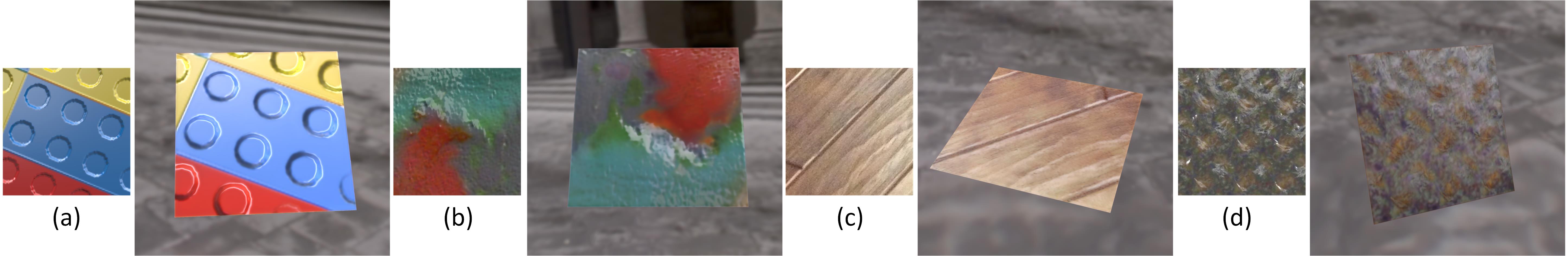
Figure 1. Physically plausible spatially varying surface appearance estimated using the proposed SA-SVBRDF-net from a single photograph of planar spatially varying plastic (a,b), wood (c) and metal (d) captured unknown natural lighting, and revisualized under a novel lighting condition.

1. Introduction

Recovering the spatially varying bidirectional surface reflectance distribution function (SVBRDF) from a single photograph under unknown natural lighting is a challenging and ill-posed problem. Often a physically accurate estimate is not necessary, and for many applications, such as large scale content creation for virtual worlds and computer games, a physically plausible estimate would already be valuable. Currently, common practice, albeit very time-consuming, is to rely on skilled artists to, given a single reference image, produce a plausible reflectance decomposition. This manual process suggests that given sufficient prior knowledge, it is possible to infer a plausible reflectance estimate for a spatially varying material from a single photograph.

Data-driven machine learning techniques have been successfully applied to a wide range of underconstrained computer graphics and computer vision problems. In this paper, we follow a similar route and design a Convolutional Neural Network (CNN) to estimate physically plausible SVBRDFs from a single near-field observation of a planar sample of a spatially varying material under unknown natural illumination. However, recovering the SVBRDF from a single photograph is an inherently ill-conditioned problem, since it is unlikely that each pixel observes a significant specular response, making it impossible to derive a full spatially varying specular component without enforcing spatial priors. We therefore estimate a reduced SVBRDF defined by a spatially varying diffuse albedo, homogeneous specular albedo and roughness, and spatially varying surface normals.

Training a CNN to estimate such a reduced SVBRDF from a single photograph under unknown natural lighting requires a large set of “labeled” photographs, i.e., with corresponding reflectance parameters. Gathering such a training dataset is often a tedious and arduous task. Currently, except for specialized materials, very few databases exist that densely cover all possible spatial variations of a material class. Unlabeled data (i.e., a photograph of a spatially varying material) is typically much easier to obtain. Each unlabeled photograph contains an instance of the complex spatially varying reflectance parameters, albeit it observed from a single view and under unknown lighting. This raises the question whether we can exploit this embedded knowledge of the spatially varying distributions to refine the desired SVBRDF-estimation CNN.

We propose, in addition to a CNN-based solution for SVBRDF estimation from a single photograph, a novel training strategy to leverage a large collection of unlabeled data –photographs of spatially varying materials without corresponding reflectance parameters– to augment the training of a CNN from a much smaller set of labeled training data. To “upgrade” such unlabeled data for training, a prediction of the unknown model parameters is needed. We propose to use the target CNN itself to generate a provisional estimate of the reflectance properties in the unlabeled photographs. However, we cannot directly use the provisional estimates and the corresponding unlabeled photograph as a valid training pair, since the estimated parameters are likely biased by the errors in the CNN, and hence it misses the necessary information to correct these errors. Our key observation is that for SVBRDF estimation, the exact inverse of the desired CNN is actually known in the form of a physically-based rendering algorithm, that given any lighting and view parameters, synthesizes a photograph of the estimated reflectance parameters. Under the assumption that the initial CNN trained by the labeled data acts as a reasonable predictor, the resulting provisional reflectance estimates represent reasonable SVBRDFs similar (but not identical) to the SVBRDFs in the unlabeled training photographs. Therefore, instead of directly using the provisional reflectance estimates and unlabeled photographs as training pairs, we synthesize a new training sample by rendering an image with the provisional reflectance estimates under random lighting and view. After refining the CNN using this synthesized training data, we can update the provisional reflectance estimates and corresponding synthetic visualizations, and repeat the process. The proposed self-augmentation training process progressively refines the CNN to be coherent with the known inverse process (i.e., rendering algorithm), thereby improving the accuracy of the target CNN. We demonstrate the efficacy of our method by training a CNN for different classes of spatially varying materials such as wood, plastics and metals, as well as perform a careful analysis and validation of the proposed self-augmentation training strategy.

2. Related Work

Single Image Reflectance Modeling

For conciseness, we focus this overview on single image reflectance modeling; for an in-depth compilation of general data-driven reflectance estimation techniques we refer to the excellent overviews by Dorsey et al. [2008] or Weinmann and Klein [2015].

In general, estimation of surface reflectance from a single photograph is an ill-posed problem. A common strategy to make estimation more tractable is to control the incident lighting during acquisition, often by limiting the lighting to a single directional light source. Wang et al. [2016] recover shape, spatially varying diffuse albedo and a homogeneous specular component from a light field observation under a single known directional light source. Xu et al. [2016] describe a general framework for recovering (piecewise constant) homogeneous surface reflectance from near-field observations lit by a known directional light source. Aittala et al. [2016] model the spatially varying surface reflectance and surface normals from a single flash image of a stationary textured material. They avoid the need for explicit point-to-point surface correspondences by relying on a powerful CNN-based texture descriptor for assessing the quality of the predictions. The Deep Lambertian Network [Tang et al., 2012] is a full end-to-end machine learning approach, based on belief networks, for jointly estimating diffuse reflectance, surface normals, and the lighting direction. Finally, in contrast to the previous methods that rely on directional light sources, Wang et al. [2011] recover the surface reflectance and complex spatially varying surface normals of a homogeneous glossy material using step-edge lighting. All these methods rely on active illumination which limits their practical use to fully controlled settings or environments with minimal ambient lighting. The proposed method does not rely on active illumination, and it does not make any assumptions on the form of the incident lighting.

Oxholm and Nishino [2012; 2016] relax the requirement of active illumination and recover the shape and homogeneous surface reflectance from a single photograph under uncontrolled, but known, lighting. Similarly, Hertzmann and Seitz [2003] recover spatially varying surface reflectance and surface normals under uncontrolled lighting given a reflectance map of each material (i.e., a photograph of a spherical exemplar under the target lighting). While these methods recover the surface reflectance from a single photograph, they do require additional measurements to obtain the required lighting/reflectance reference maps.

Romeiro and Zickler [2010] assume the incident lighting is unknown, and propose to recover the most likely reflectance of a spherical homogeneous object under the expected natural lighting distribution. Similarly, Lombardi and Nishino [2012; 2016] express the reflectance recovery of a homogeneous object under unknown lighting as a maximum a-posteriori estimation with strong priors on both lighting and surface reflectance. Barron et al. [2015] propose to find the most likely shape, piecewise constant spatially varying diffuse reflectance, and illumination that explains the input photograph based on strong hand-crafted priors on each component. Rematas et al. [2016] employ a convolutional neural network to extract homogeneous reflectance maps under unknown lighting and shape. All these methods are limited to either diffuse or homogeneous materials. The proposed method on the other hand, is specifically designed for spatially varying materials.

Finally, AppGen [Dong et al., 2011] takes a different approach to separate the different reflectance components from a single photograph by putting the user in the loop. While AppGen greatly accelerates the authoring process, it does not scale well to large-scale content generation due to the required (albeit limited) manual interaction. Furthermore, AppGen assumes the input image is illuminated by a single directional light.

Deep Learning with Unlabeled/Synthetic Data

Recent advances in deep learning have been successfully applied to a wide variety of computer graphics and computer vision problems. A full overview falls outside the scope of this paper, and we focus our discussion on prior work that combines deep learning techniques with unlabeled and/or synthetic training data.

A common weakness for many deep learning methods is their reliance on large training datasets which can be difficult and/or time-consuming to obtain. To alleviate the difficulty in gathering such datasets, several researchers have looked at synthetic data to fill in the gaps. Synthetic data has been used to improve the training of various tasks, for example for: text detection [Gupta et al., 2016], hand pose estimation [Tompson et al., 2014], object detection [Gupta et al., 2014], semantic segmentation of urban scenes [Ros et al., 2016], etc. Gaidon et al. [2016] showed that pretraining on synthetic data improves the overall accuracy of the regression. Narihira et al. [2015] propose “Deep IntrinsicNet”, a CNN for single image intrinsic decomposition; a subject closely related to reflectance estimation, and which decomposes an image in its “shading” and “reflectance” components. They observe that marrying synthetic training data with CNNs is a powerful paradigm, and follow Chen et al. [2013] to train their IntrinsicNet using the MPI Sintel dataset. We also rely on synthetic training data, but instead of only synthesizing training data, we also use it to complete non-synthetic unlabeled training data.

Shelhamer et al. [2015] also rely on CNNs to infer the intrinsics from a single image. However, they note that CNNs cannot guarantee physical coherence, and propose to combine and jointly train a CNN for surface normal estimation together with a fixed inverse rendering pipeline to compute the intrinsic decomposition (e.g., using the method of Barron et al. [2015]). The proposed method also includes a rendering component, but instead of appending an inverse rendering pipeline to the CNN, we employ a forward rendering pipeline to aid in training by synthesizing new training pairs from unlabeled data.

Breeder Learning [Nair et al., 2008] relies on a known generative black-box function to generate novel training data by perturbing the estimated parameters, and computing the resulting exemplar using the black-box generator. In contrast, self-augmentation (where the forward rendering component could be seen as a generative black-box) relies on unlabeled data instead of perturbations to explore and refine the search space. Furthermore, perturbations in the parameter space do not necessarily match the real-world distribution of the underlying data, especially for high-dimensional parameter spaces (e.g., a random perturbation on the diffuse albedo or on the surface normals does not necessarily yield a valid SVBRDF within the targeted material class).

3. SVBRDF-Net

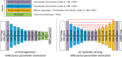
Figure 2. Network structure. Left: the network structure for homogeneous reflectance parameters consists of an analysis subnetwork of convolution and pooling layers, followed by a fully connected synthesis network with $1024$ hidden variables. Right: the network for spatially varying reflectance parameters consists of an identical analysis network of convolution and pooling layers, followed by a synthesis upsampling network that mirrors the analysis network. To reintroduce high frequency details during upsampling, the feature maps from the analysis layers are concatenated to the corresponding synthesis layers (illustrated by the red links).

Convolutional Neural Network Configuration

Our goal is to estimate plausible appearance parameters from a single photograph of a near-field observation of a planar material sample under unknown natural lighting. Modeling both spatially varying diffuse as well as specular reflectance from a single photograph is an ill-posed problem. We therefore reduce the complexity by assuming a homogeneous constant specular component on top of a spatially varying diffuse component and surface normals. We introduce a convolutional neural network solution (SVBRDF-net) to learn the mapping from a photograph of a spatially varying material to appearance parameters, where the homogeneous specular component is represented by the Ward BRDF model [Ward, 1992] parameterized by its specular albedo ${\rho_{s}}$ and specular roughness parameter ${\alpha}$, the spatially varying diffuse component is modeled by a per-pixel diffuse albedo ${\rho_{d}}(x)$, and the surface normals are encoded as a 3D vector per pixel $n(x)$:

(1) $${f_{r}}({\omega_{i}},{\omega_{o}},x)=\frac{{\rho_{d}}(x)}{\pi}+{\rho_{s}}\frac{{e^{-\tan^{2}\delta/{\alpha}^{2}}}}{4\pi{\alpha}^{2}\sqrt{{({\omega_{i}}\cdot n(x))}{({\omega_{o}}\cdot n(x))}}},$$

where $\delta$ the angle between the halfway vector ${\omega_{h}}=({\omega_{i}}+{\omega_{o}})/||{\omega_{i}}+{\omega_{o}}||$ and the normal $n(x)$. Note that the proposed SVBRDF-net is not married to the Ward BRDF model and any other BRDF model can be used instead.

Due to the inherent scale-ambiguity between the overall intensity of the lighting and surface reflectance (i.e., scaling the intensity of the lighting can be compensated by dividing the diffuse and specular albedo by the same factor), SVBRDF-net can only estimate relative diffuse albedos ${\rho_{d}}_{rel}$ and the relative specular albedo ${\rho_{s}}_{rel}$. We will assume without loss of generality that the average diffuse albedo (over all color channels) is fixed ($avg({\rho_{d}})=0.5$), and that the relative diffuse and specular albedo are expressed with respect to this average diffuse albedo: ${\rho_{d}}_{rel}(x)={\rho_{d}}(x)/s$, ${\rho_{s}}_{rel}={\rho_{s}}/s$ and $s=2avg({\rho_{d}})$. Consequently, any uniform scaling applied to ${\rho_{d}}$ and ${\rho_{s}}$ does not affect ${\rho_{d}}_{rel}$ and ${\rho_{s}}_{rel}$. For stability, we use the logarithm of the relative specular albedo (${\rho_{s}}_{log-rel}=\log{{\rho_{s}}_{rel}}$) to avoid huge parameter values for the specular component in SVBRDF-net when the absolute average diffuse albedo ($s$) is small. Furthermore, to ensure a more uniform distribution with respect to the error on the appearance, a log-transformation is also applied to the specular roughness encoded in SVBRDF-net: ${\alpha}_{log}=\log{{\alpha}}$.

The proposed SVBRDF-net is a union of separate network structures; one for the homogeneous parameters (relative (log) specular albedo and (log) roughness), and another for the spatially varying parameters (relative diffuse albedo and surface normals). Figure 2 depicts the network structure and lists the relevant dimensions of the layers. The number of layers and convolution/upsample filter sizes are similar to those used in prior work (e.g., [Rematas et al., 2016]). Both networks share the same analysis subnetwork structure consisting of a series of convolution layers and pooling layers. Each convolution layer is followed by a batch-normalization layer [Ioffe and Szegedy, 2015] and a ReLU activation layer. This analysis subnetwork reduces the input photograph to the essence needed for estimating the relevant model parameters. The analysis subnetwork is followed by a different synthesis subnetwork for each output parameter type:

• Homogeneous Specular Albedo and Roughness: are synthesized by adding a fully connected layer with 1024 hidden variables, and $6$ output nodes (i.e., relative (log) specular albedo ${\rho_{s}}_{log-rel}$ and (log) roughness ${\alpha}_{log}$ estimates per color channel).

• Spatially Varying Diffuse Albedo: is synthesized by a set of upsample+convolution layers (often misnamed as a “deconvolution” layer). Similarly as for analysis, each layer is followed by a batch normalization and ReLU layer before a bilinear upsampling step. As in [Rematas et al., 2016; Ronneberger et al., 2015], we concatenate feature maps from the corresponding analysis layers (marked by the red links in Figure 2) to help reintroduce high frequency details lost in subsequent convolution layers during analysis. The final output is mapped to the proper range (i.e., $[0,1]$) using a standard per-pixel fixed sigmoid function. As batch normalization does not work well with a sigmoid output layer, we omit the batch normalization at the final output layer.

• Spatially Varying Normal Map: is synthesized by an identical (but separate) network as for the diffuse albedo.

We train a separate analysis-synthesis network for each output parameter type.

Training by Self-Augmentation

One of the main challenges in training the proposed SVBRDF-net, is to obtain a sufficiently large training dataset that captures the natural distribution of all spatial variations for the target material class. For each spatial variation, we need, in addition, a sufficient sampling of the different viewing and lighting conditions. Essentially, the search space we are regressing is the outer product of the appearance variations due to spatial variations in reflectance properties, different natural lighting conditions, and differences in viewpoint. The latter two dimensions are common over different material classes and are relatively easily to sample. The former, on the other hand, is highly dependent on the material type and is ideally sampled through diversity in the training data.

The desired labeled training data in the case of SVBRDF-net is in the form of a photograph of a planar sample of an spatially varying material under an unknown natural lighting condition paired with the corresponding model parameters (i.e., spatially varying relative albedos, log-roughness, and surface normals). Note that the high cost of obtaining labeled training data is solely due to the cost of the necessary acquisition/authoring process to obtain the model parameters. On the other hand, the cost to obtain unlabeled data in the form of a photograph of a planar spatially varying material is significantly smaller. Similarly to labeled data, such unlabeled data represents samples in the search space, except that the corresponding model parameters are unknown. Now suppose we have an oracle that can predict these model parameters from the unlabeled data, then we can use the unlabeled data in conjunction with the prediction to refine SVBRDF-net. Of course, this oracle is exactly the network we desire to train. Now let’s assume we have a partially converged SVBRDF-net, trained from a smaller set of labeled training data. This partially converged network forms an approximation of the desired oracle. Hence, we can use the network itself to generate provisional model parameters for each unlabeled exemplar. However, we cannot directly use these provisional model parameters paired with the input unlabeled image for training since the provisional model parameters are biased by the errors in the partially converged network (and thus cannot correct these errors).

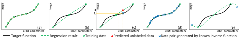
Figure 3. Illustration of the Self-Augmentation Training Process. (a) Given sufficiently dense sampled training data, the target manifold can be well modeled. (b) However, when insufficiently sampled, the target network only provides a coarse approximation. (c) Self-augmentation exploits the fact that a forward rendering algorithm provides an exact inverse of the target manifold. Given a coarse approximation of the manifold, we can make a provisional estimate of the reflectance parameters of an unlabeled image (marked with ’U’). Rendering the estimated provisional parameters from a new viewpoint and under novel lighting, produces a different image (’R’) than the unlabeled image. However, unlike the unlabeled image, this rendered image is not biased by the approximation error of the coarse network. When inputting this rendered image to the target CNN, we obtain a different estimate of the parameters than the ones used for rendering. Self-augmentation attempts to reduce the mismatch between the provisional and estimated parameters from the rendered image, thereby indirectly improving the accuracy of the target network. (d) Repeatedly applying the self-augmentation process on a large set of unlabeled data points, should yield a progressively more accurate approximation of the target network. (e) However, care must be taken that the unlabeled data points lie in or near the search space covered by the labeled data points as the latter determines the range in which the initial coarse approximative network is well-defined.

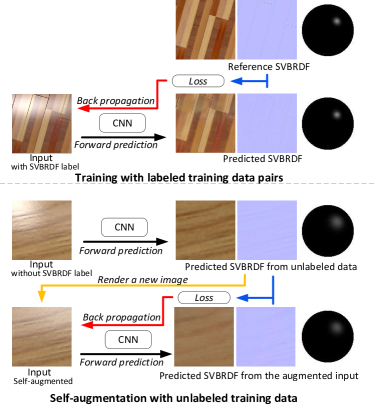
Figure 4. Summary of the Self-augmentation Training Process. First, an initial approximative network is trained using only labeled data. Next, we alternate between training on labeled and unlabeled data. For each unlabeled exemplar, we estimate provisional reflectance parameters, and synthesize a new (temporary) labeled training pair by rendering a corresponding exact visualization. This new labeled training pair, is then used to further refine the network.

Our key observation is that the exact inverse of the target network is known in the form of a rendering algorithm, i.e., given the lighting and view parameters together with the model parameters, we can synthesize a photograph of the SVBRDF. Our goal is to exploit this (inverse) knowledge of the search space to refine the regression of the CNN. Assuming a locally smooth search space, and assuming the unlabeled data lies in the search space covered by the labeled training data (i.e., the labeled data covers the full target search space), then the provisional model parameters should approximately follow the target distribution. Hence the extracted spatially varying model parameters form a plausible SVBRDF (albeit not necessarily the same as the ground truth physical parameters of the unlabeled data exemplar). Thus, the provisional model parameters and a corresponding synthesized visualization under either the same or different lighting and view conditions, provide a valid labeled training exemplar that can be used to refine the CNN. This process is illustrated in Figure 3. Given sufficient training data (a), we can accurately capture the target search space’s manifold. However, when a smaller labeled training set is used (b), the resulting regression only forms a coarse approximation. Given unlabeled data (marked by ’U’ on the vertical axis in (c)), we can estimate provisional model parameters using the initial network as an oracle (the corresponding projection on the CNN is marked by a triangle). The rendering process takes these provisional model parameters and ’projects’ them back to image space over the exact manifold, resulting in a different rendered image (marked by ’R’ on the vertical axis). When using this synthetic pair for training, we observe a discrepancy between the estimated model parameters from this synthetic image (i.e., the projection of the synthetic rendering (’R’) over the CNN (dashed line)) and the initial provisional model parameters. Hence, the training process will minimize this discrepancy. Assuming local smoothness over the search space and assuming that the initial CNN prediction is relatively close to the target manifold, minimizing this discrepancy should locally pull the CNN’s manifold approximation closer to the desired search space’s manifold (d). However, care must be taken to ensure that the unlabeled data resides in or near the search space covered by the labeled training data (e), as there is no guarantee about the extrapolation behavior of the CNN outside this region, and thus the provisional model parameters are unlikely to represent a plausible SVBRDF in the targeted material class and/or potentially correspond to a folding of the manifold (thereby creating ambiguities in the training).

We coin our training strategy “self-augmenting” since it relies on the exactness of the inverse model (i.e., the rendering algorithm) to guide the training, and the CNN itself to provide reasonable model parameters. We integrate this self-augmentation in the training process, and repeatedly apply it on the progressively refined network (and thus with progressively improved provisional model parameters). We will use the short-hand notation SA-SVBRDF-net to refer to the self-augmented SVBRDF-net, and use SVBRDF-net to refer to the regularly trained SVBRDF-net (i.e., without self-augmentation).  Figure 4 summarizes the proposed self-augmentation training strategy.

4. Results

Implementation

We implement the proposed SVBRDF-net detailed in Section 3 in Caffe [Jia et al., 2014] using a constant initialization strategy and train it with ADAM [Kingma and Ba, 2015]. We first produce an initial CNN by training, from scratch, with labeled data only for $10$ epochs. Next, we self-augment this initial SVBRDF-net using the unlabeled training data. However, whereas labeled data provides absolute cues to the structure of the search space, the unlabeled data only constrains the local structure of the search space (i.e., it ensures that the network is locally consistent with the rendering process). Therefore, care should be taken to ensure that the self-augmentation does not steer the network too far from the labeled data, and avoid collapsing the network to a (self-coherent) singular point. Hence, we interleave the training after each randomly selected unlabeled mini-batch, with a random labeled mini-batch that biases the training to remain faithful to the labeled data. Table 1 summarizes all relevant training parameters. For all results in this paper, we trained the proposed SA-SVBRDF-net for an input resolution of $256\times 256$.

Table 1. Summary of Training Hyperparameters. We use the default Caffe values for unlisted parameters.

Learning rate			Weight	Momentum	Mini-batch
Inital	Policy	Gamma	decay		size
0.002	Inverse	$10^{-4}$	$10^{-4}$	0.9	16

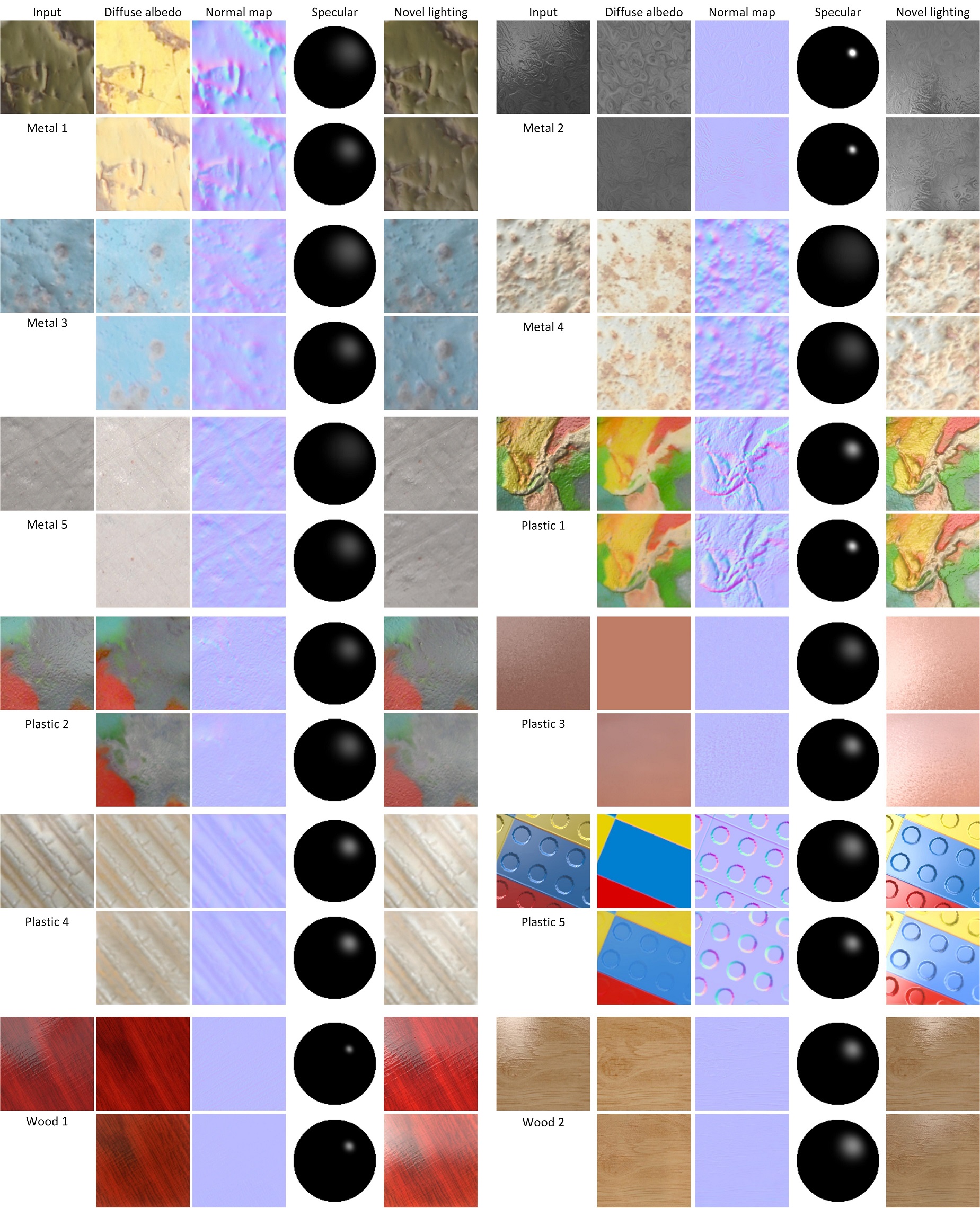
Figure 5. Qualitative Comparison to Reference Reflectance Parameters. Reflectance parameters obtained with the wood, plastic, and metal SA-SVBRDF-nets (odd rows) compared to reference reflectance parameters (even rows). Each row shows (left to right), spatially varying relative diffuse albedo, normal map, the homogeneous relative specular albedo and roughness mapped on a sphere and illuminated by a directional light source, and a visualization of the reference/estimated appearance parameters under a novel lighting condition.

Data Collection & Preprocessing

We source SVBRDF-data for spatially varying wood, plastics, and metals from an online material library [VRay, 2016], supplemented by artist generated SVBRDFs. We average specular albedo and roughness when the dataset provides spatially varying specular albedo or roughness. The wood dataset contains $50$ SVBRDFs, the plastic dataset contains $60$ SVBRDFs and the metal dataset contains $60$ SVBRDFs. We randomly select $10$ SVBRDFs from each dataset for testing, and retain the remainder for training (thus $40$ for wood, and $50$ for plastic and metal). To generate labeled training/test data, we furthermore gather $50$ HDR light probes [HDRLabs, 2016], and render (with a GPU rendering implementation that correctly integrates the lighting from the full hemisphere of incident directions) each SVBRDF under $40$ selected light probes for the training set, and the remaining $10$ probes for the test set, for $9$ randomly selected rotations. Consequently, the lighting for each labeled training pair, as well as the test set, is different. During training, we randomly crop and rotate a $256\times 256$ window from the rendered images to sufficiently sample the rich texture variations. As we aim for a practical tool, we only use radiometrically linearized “low” dynamic range images (i.e., all pixel values are clamped to the $[0,1]$ range). If the input image is not radiometrically linear, we apply a gamma (2.2) correction before feeding it to the proposed SA-SVBRDF-net.

Unlabeled data is gathered from OpenSurface [Bell et al., 2013], as well as internet images collections. In total, the number of unlabeled images are $1000$, $1000$, and $1200$ for wood, plastic and metal SA-SVBRDF-net training respectively. During self-augmentation, we randomly pick and rotate a lighting environment for generating the provisional labeled training pair using the same rendering algorithm as was used for generating the training data. We assume that both the labeled and unlabeled training data are drawn from the same distribution. However, both (labeled and unlabeled) databases are likely to be gathered from different sources or created through a different authoring process. Consequently, their respective inherent distribution through the search space might differ. To avoid biasing the training, we select a subset from the unlabeled data such that it mimics the distribution of the labeled data. However, we do not know the reflectance parameters for the unlabeled data, and thus also not their distribution. Instead, of matching the search space distribution, we match the first order statistics of the images as a proxy. Practically, we create the histogram of the average colors of the labeled training images, and then randomly select the subset of the unlabeled images such that the resulting histogram follows the same distribution. While a crude approximation, we have found this to work well in practice. Furthermore, we auto-expose the rendered synthetic images before clamping pixel values to the $[0,1]$ range. This allows us to directly use the relative albedos during rendering instead of converting them to absolute parameters; any scale applied to both the relative diffuse and specular albedo is compensated for by a corresponding change in the auto-exposure.

As noted in Section 3, to resolve the ambiguity between the intensity of the lighting and the reflectivity of the surface, we ensure that the average diffuse albedo over all color channels equals 0.5, and express the specular albedo with respect to this average. However, a related ambiguity still exists between the color of the lighting and the material. We cannot simply set the average diffuse albedo for each color channel to $0.5$ as this would result in a complete loss of material color. Instead, when generating labeled training samples, we white-balance the lighting such that the irradiance is color neutral:

(2) $$\forall i,j\in[r,g,b]:s_{i}=s_{j},~{}\text{and}~{}~{}s_{r,g,b}=\int_{\Omega_{+}}E({\omega_{i}})\cos{\theta_{i}}d{\omega_{i}},$$

where $E({\omega_{i}})$ is the incident lighting. In addition, we also assume that unlabeled data and/or input photographs are (approximately) correctly white balanced. In other words, we assume that the diffusely reflected color observed in the input photograph has the same color as the diffuse albedo.

Results

Figure 1 shows a series of input photographs for the wood, plastic, and metal SA-SVBRDF-nets and a revisualization under a novel lighting condition for the recovered spatially varying reflectance parameters. Qualitatively, we argue that the appearance of the revisualizations exhibits the same visual qualities as the input photographs. This suggests that the proposed SA-SVBRDF-nets are able to estimate plausible reflectance parameters.

While our goal is to model plausible surface reflectance from a single photograph, it is nevertheless informative to explore how well the estimated parameters match ground truth surface reflectance parameters. Figure 5 shows a comparison between ground truth reflectance parameters and the estimated parameters obtained with the wood, plastic, and metal SA-SVBRDF-nets. For each example, we show two rows, where the top row shows the ground truth and the bottom row shows the recovered results. For each row, we show (from left to right), the input photograph under an unknown natural lighting condition, the recovered diffuse albedo, the recovered normal map, the homogeneous specular component mapped on a sphere and lit by a directional light, and a visualization under a novel lighting condition. Note that none of the input photographs/SVBRDFs were included in the training set to avoid bias in the results. While there are some differences, overall, the estimated reflectance parameters match the reference parameters well. This further confirms that the resulting reflectance parameters estimated with SA-SVBRDF-net are physically plausible.

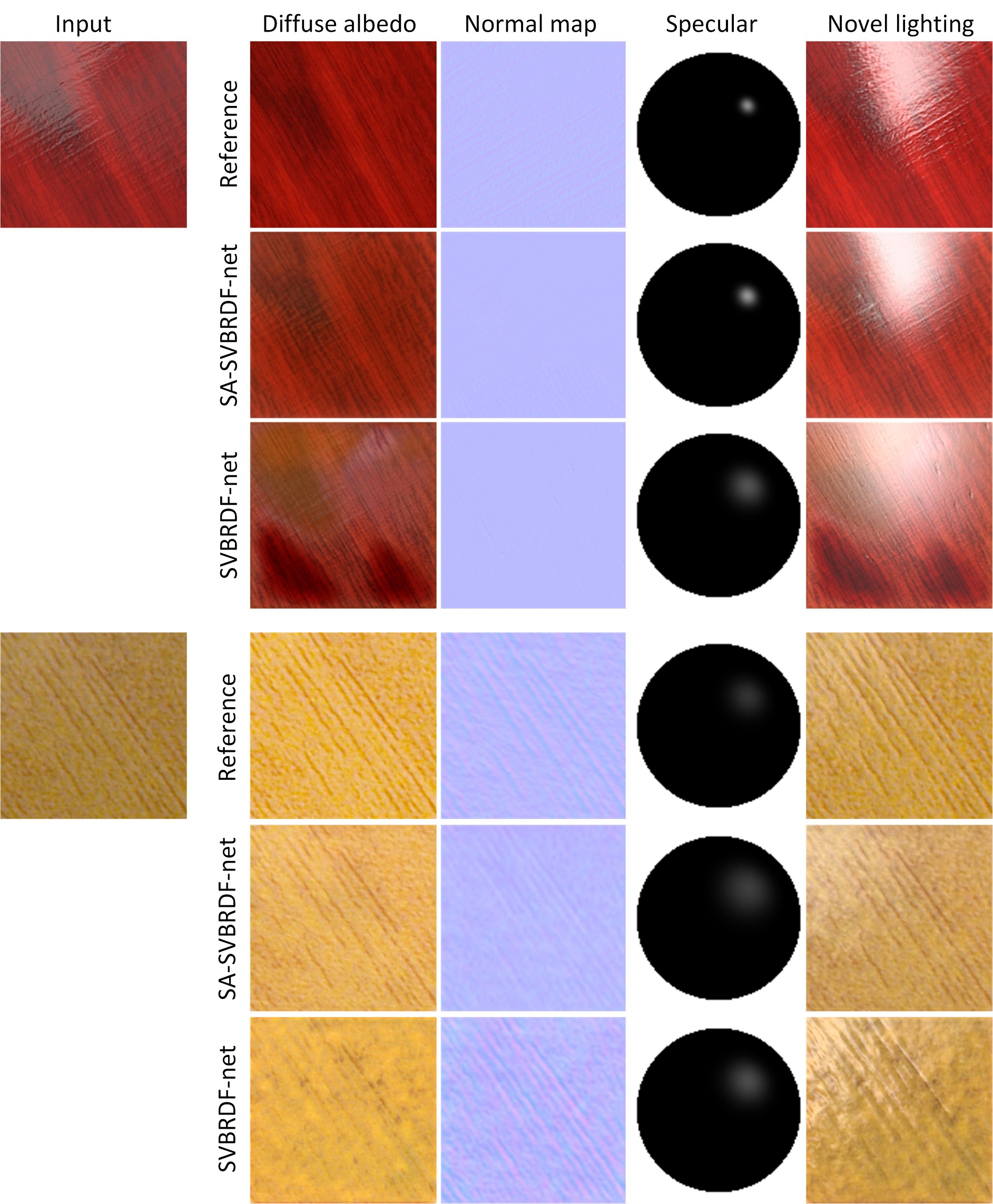
Figure 6. Impact of Self-Augmentation. A qualitative comparison between reflectance parameters estimated with SVBRDF-net trained with and without self-augmentation. The SA-SVBRDF-net estimates appear more plausible and exhibit less artifacts than the results from the regular SVBRDF-net.

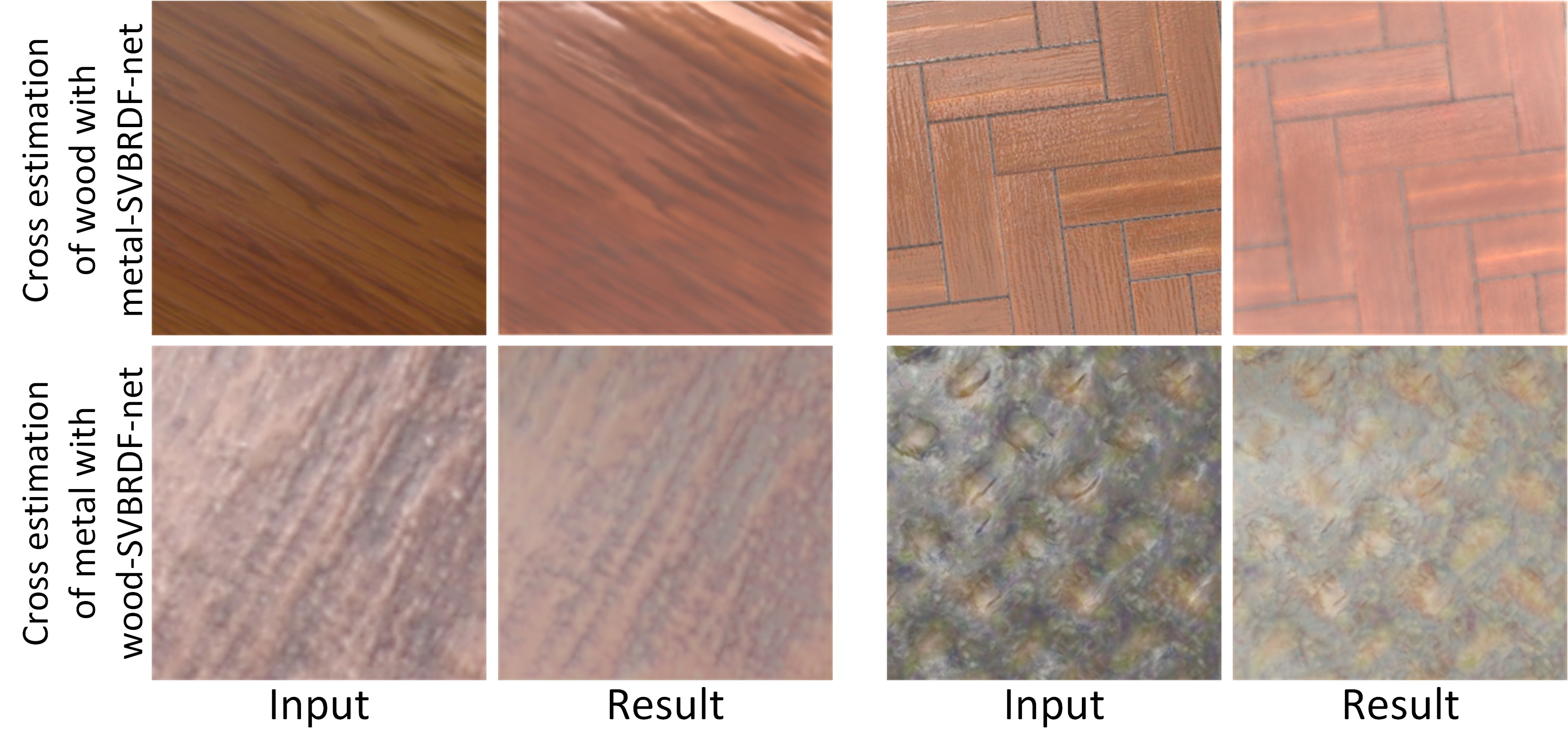
Figure 7. Cross Estimation. Surface appearance of wood and metal estimated using an SVBRDF-net trained on another material class (metal and wood respectively) fails to produce physically plausible results.

Figure 6 compares the estimated reflectance estimates of the wood SVBRDF-net and SA-SVBRDF-net. In both cases, we use exactly the same set of $40$ labeled training samples. Compared to the regular SVBRDF-net, the proposed SA-SVBRDF-net trained with self-augmentation produces qualitatively more plausible results with less visual artifacts. For example, the top example includes remnants of the specular highlight from the input photograph in the diffuse albedo while overestimating the specular roughness, and the bottom example exhibits a faint “splotchy” structure in the diffuse albedo. This empirically shows that the proposed self-augmentation strategy greatly helps the convergence of the training process, and significantly reduces the required number of labeled training samples. Both networks were trained on a NVidia Titan X (Maxwell) for $20$ epochs; $10$ epochs to obtain the rough initial SVBRDF-net, and then an additional $10$ with-out/with unlabeled data for the SVBRDF-net and SA-SVBRDF-net respectively. Total training time without self-augmentation took $30$ hours, and $38$ hours with self-augmentation. Evaluating the (SA-)SVBRDF-net is very fast and only takes $0.3$ seconds on a GPU.

Our SA-SVBRDF-nets are trained for a specific material type, and there is no guarantee on the quality of the results when a input photograph of a different material is provided. Figure 7 shows a result of feeding a spatially varying wood material in the metal SA-SVBRDF-net, and vice versa. As expected, the resulting cross estimation fails to produce physically plausible results. Similarly, SA-SVBRDF-net expects spatially varying materials with a homogeneous specular component. We empirically observe (Figure 8) that if the spatial variations in the specular component are modest, SA-SVBRDF-net still produces a plausible result. However, when faced with significant spatial variations, the result is often unpredictable.

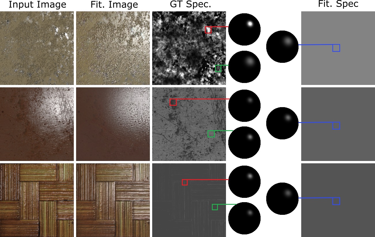
Figure 8. Spatially Varying Specular Component While SVBRDF-net expects and estimates a homogeneous specular component, it can still robustly estimate a plausible specular component when the spatial variations are modest.

5. Discussion

Our results show that the proposed SA-SVBRDF-net can decompose a photograph of a planar spatially varying sample under unknown distant lighting in its reflectance components. Key to our method is the self-augmentation training strategy. In this section, we further explore the benefits, assumptions, and limitations of the proposed self-augmentation procedure.

BRDF-net

To validate the proposed self-augmentation training strategy we introduce a CNN-based solution to the related, but less complex, problem of estimating the homogeneous BRDF from a single image of a smooth spherical object under unknown natural lighting conditions. For validation purposes, we limit the experiment to estimating monochrome BRDFs from a single monochrome image under monochrome lighting. The advantage of validating the self-augmentation training strategy on a homogeneous BRDF-net is that we can easily enumerate the full search space, allowing us to synthesize labeled training data and visualize the learned and ground truth manifolds and corresponding errors.

We employ the same network structure as the (log) roughness and (log-relative) specular albedo prediction network in the previously proposed SVBRDF-net. We express the relative specular albedo as ${\rho_{s}}_{rel}={\rho_{s}}/{\rho_{d}}$ instead of with respect to the average diffuse albedo as in SVBRDF-net.

We generate a training set by uniformly sampling $10$ diffuse and specular albedos in the $[0.05,1.0]$ range, and $15$ roughness samples log-uniformly sampled in $[0.02,1.0]$, yielding a total of $1500$ training samples. We also define a test set for evaluating the errors by selecting samples mid-distance between any two consecutive training samples; these are the sample points furthest away from the training samples, which are expected to contain the largest error.

Because the specular-diffuse ratio estimated by the BRDF-net cannot be used directly for synthesizing a provisional training image during self-augmentation, we randomly select a diffuse/specular albedo pair for rendering such that the posterior distribution is uniform.

Validation

To quantify the impact of self-augmentation on the accuracy of BRDF-net, we regress a reference baseline BRDF-net on the full labeled training set that densely and uniformly covers the full search space. We measure the reconstruction error as the mean squared error between visualizations of the ground truth and estimated reflectance parameters under the same view and lighting conditions as the input image. Reducing the size of the training dataset when regressing the BRDF-net without self-augmentation, dramatically decreases the accuracy (Figure 9 top row). We consider two different subsampling strategies: uniformly reducing the sampling rate of (diffuse and specular) albedo and roughness (i.e., effective sampling rates: $5\times 5\times 7$, $3\times 3\times 5$, and $2\times 2\times 2$), and randomly selecting a subset from the full training set (of size: $12.5\%$, and $3.7\%$; see Figure 9 bottom row). Compared to the baseline we observe a correlation in the error distribution with the subsampling scheme – regions with low training data density exhibit larger error. When using the same subsampled training sets in conjunction with self-augmentation, where the unlabeled image set equals the images left out from the labeled training set, we observe an error rate similar to the baseline BRDF-net (Figure 9 middle row). Surprisingly, even in the extreme case where we only provide the corners of the parameter space (i.e., $2\times 2\times 2$ sampling rate), the resulting SA-BRDF-net still achieves accurate BRDF estimates.

Table 2. Labeled-Unlabeled Training Data Ratio. The error for different ratios of labeled and unlabeled data randomly sampled from the densely sampled search space.

Percent.	No Self-	Percentage Unlabeled
Labeled	augmentation	5	10	20	30	50	70	80	90	95
5	0.002549	0.001395	0.001141	0.000884	0.000689	0.000704	0.000651	0.000578	0.000592	0.000628
10	0.001252	0.001382	0.001027	0.000720	0.000760	0.000671	0.000584	0.000634	0.000592
20	0.000746	0.001155	0.000845	0.000751	0.000621	0.000619	0.000641	0.000513
30	0.000662	0.000714	0.000648	0.000694	0.000492	0.000548	0.000535
50	0.000562	0.000660	0.000559	0.000552	0.000506	0.000470
70	0.000619	0.000601	0.000462	0.000550	0.000499
80	0.000553	0.000542	0.000421	0.000413
90	0.000546	0.000505	0.000471
95	0.000550	0.000471
100	0.000499

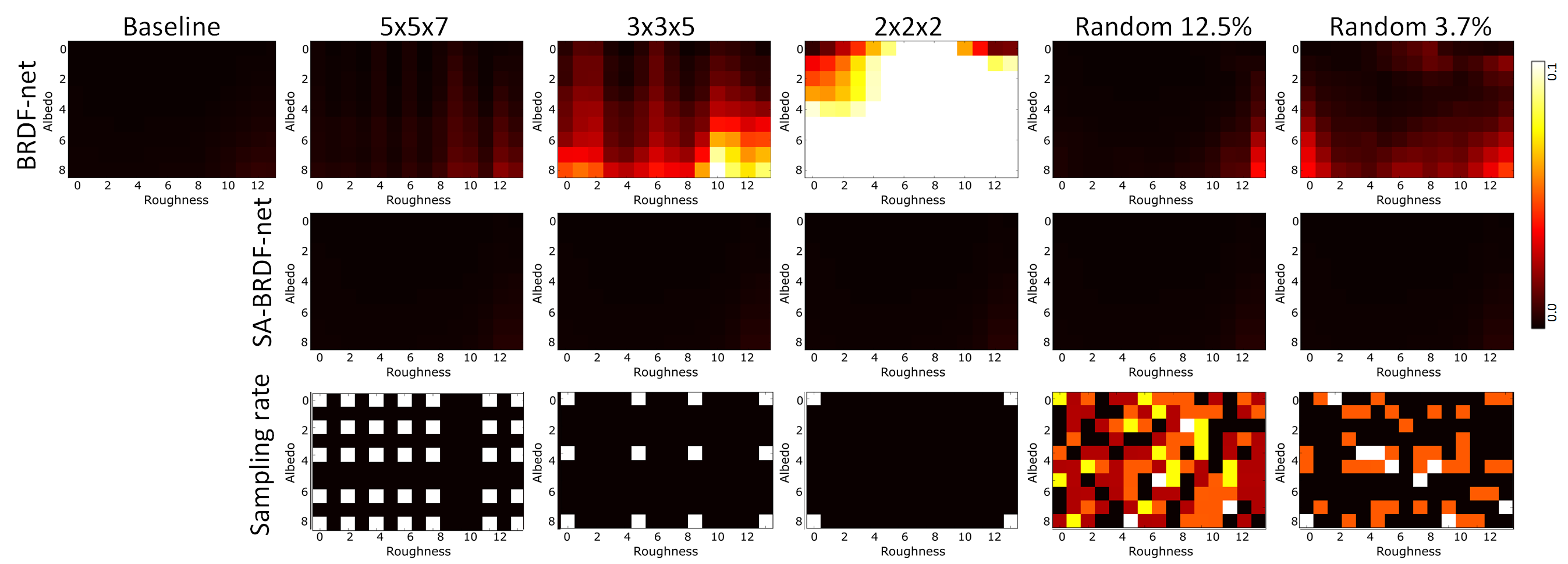
Total Mean Squared Error
Subsample Rate	BRDF-net	SA-BRDF-net
Baseline	$0.0004$
$5\times 5\times 7$	$0.0010$	$0.0004$
$3\times 3\times 5$	$0.0060$	$0.0005$
$2\times 2\times 2$	$0.1001$	$0.0005$
Random $12.5\%$	$0.0007$	$0.0004$
Random $3.7\%$	$0.0029$	$0.0004$

Figure 9. Self-augmentation Validation on BRDF-net. Error plots over the search space of (homogeneous) BRDF-net for different subsampling rates for the labeled training data. The reconstruction error is assessed on visualizations of the reference and estimated reflectance parameters. For visualization purposes, we integrate the 3D search space over the specular albedo axis, and plot the resulting value for each diffuse albedo / specular roughness combination. Top-left: baseline error on BRDF-net regressed over densely sampled training data. Top-row: the reconstruction error for different subsampling rates (uniform subsampling of diffuse albedo, specular albedo, and specular roughness at $5\times 5\times 7$, $3\times 3\times 5$ and $2\times 2\times 2$ sample rates, and randomly selecting samples that cover $12.5\%$ and $3.7\%$ of the search space). Middle-row: corresponding reconstruction error for SA-BRDF-net (i.e., trained with self-augmentation). Bottom-row: visualization of the sampling pattern. Right: total error over the full search space for each subsampling case.

In the above experiment the sum of the labeled and unlabeled training data densely covers the full search space. To better understand the trade-offs between the number of labeled versus unlabeled training data, we compare the error of different BRDF-nets trained on varying ratios of labeled and unlabeled training data (uniformly) covering different percentages of the densely sampled search space (Table 2). Note, we consider $450$ randomly selected lighting conditions per labeled training exemplar, and only a single randomly selected lighting condition per unlabeled training exemplar – increasing the number of lighting conditions for each unlabeled training sample did not improve the error because self-augmentation synthesizes a new provisional training exemplar under a random lighting condition and thus automatically samples the different lighting conditions already. From this experiment we can see that, as expected, the accuracy improves for increased number of labeled and/or unlabeled training exemplars. However, care must be taken when comparing the percentages of labeled versus unlabeled training exemplars in Table 2 as these indicate coverage of the search space and not number of images ($450$ lighting conditions versus a single lighting condition for labeled and unlabeled training exemplars respectively). Furthermore, we also observe that self-augmentation is most advantageous when the number of labeled training images is low; when the number of labeled training images is large, the accuracy of SVBRDF-net is already good, and there is only limited room for improvement. We argue that a significant portion of the training data in regular CNN training merely aids in refining the approximation of the search space, and only a small portion is required to span the search space. Consequently, care must be taking to ensure that the selection of the labeled training data exhibits sufficient diversity and fully spans the intended search space, especially for very small labeled training sets.

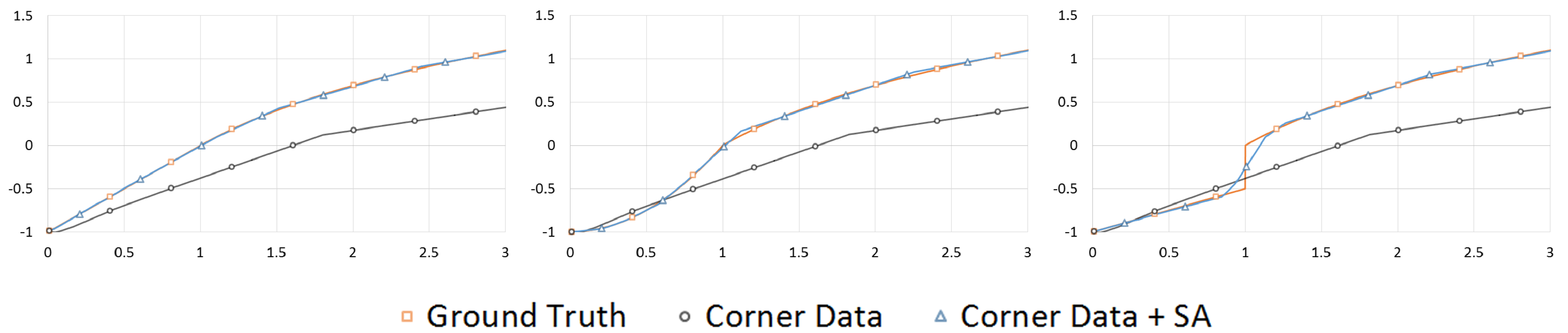
Figure 10. Impact of Discontinuities in search space illustrated on a 1D curve regression with labeled data only located the two ends. While self-augmentation assumes a locally smooth search space, it still improves the overall accuracy on a discontinuous search space, albeit smoothing out the discontinuity.

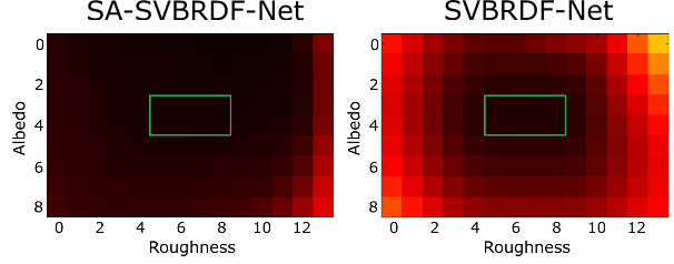
Figure 11. Extrapolation. The extrapolation behavior improves for a BRDF-net trained with labeled data constrained to the center region (green box) when self-augmented with unlabeled data covering the full search space.

Practical Implications of Assumptions

Self-augmentation assumes the search space is locally smooth, and no “jumps” or discontinuities occur in the space. In other words, the inverse of the targeted CNN should be well-defined. Intuitively, unless the location of the discontinuity is precisely determined by the labeled training data, the projection of the unlabeled data will exhibit a large error depending to which side of the discontinuity the estimate is biased toward. Depending on local gradients, it is possible that self-augmentation drives the search space to an (incorrect) local minimum. Figure 11 illustrates the effect of a non-smooth search space on a simple 1D curve regression with only two labeled training exemplars located the ends of the range, and the unlabeled data distributed through the full space. As can be seen, while self-augmentation significantly improves the accuracy, it tends to smooth out the discontinuity.

Self-augmentation also assumes that the unlabeled training data lies in the region of the search space covered by the labeled training data and no guarantees can be made on the accuracy outside the covered search space (i.e., extrapolation). However, empirically we found that in many cases, self-augmentation also improves accuracy beyond the covered region (Figure 11). Consequently, reliable estimates can still be obtained in practice as long as we restrict unlabeled data and queries to lie close to the region covered by the labeled data.

Limitations

While the proposed SA-SVBRDF-net is able to recover plausible reflectance parameters from a single photograph under unknown natural lighting, the network is limited by the training data. Each SA-SVBRDF-net is trained for a particular material class. Consequently, for each new material type, a new network needs to be trained. Similarly, the quality of the appearance estimates obtained with the proposed SA-SVBRDF-net are also limited by information contained in the input photograph. If a particular reflectance feature is not or limited present in the input image (e.g., specular highlight), then the corresponding estimated reflectance parameters will deviate more from the ground truth.

The proposed SA-SVBRDF-net is restricted to planar material samples under distant lighting, and with a homogeneous specular component. Generalizing SA-SVBRDF-net to unknown varying geometries and/or local lighting conditions and/or spatially varying specularities is non-trivial due to the ill-posed nature of the problem and the huge search space.

While we have shown empirically that self-augmentation can greatly reduce the required amount of labeled training data, a formal theoretical derivation on the conditions for convergence, and the conditions on the distribution of labeled/unlabeled data are missing.

Relation to other Deep Learning Methods

The proposed method shares conceptual similarities to other recent deep learning methods. Generative Adversarial Networks (GAN) [Goodfellow et al., 2014] train two competing networks: a generating network that synthesizes samples and a discriminative network that attempts to distinguish real and synthesized samples. Self-augmentation also relies on a “synthesizer”, except that in our case it is a fixed function. Similarly, Variational Auto-Encoders (VAE) [Kingma and Welling, 2014] train an end-to-end encoder and decoder. The latent variables are parameterized with (Gaussian) models, and variations of the search space are explored by sampling these models. The proposed solution also explores the search space by random sampling of parameters (i.e., lighting and view). However, we desire parameters with a precise physical meaning; the unsupervised nature of VAEs make it difficult to generate models (i.e., parameters) with physical meaning, even with conditional variants such as CVAE [Sohn et al., 2015] or CGAN [Liu and Tuzel, 2016].

6. Conclusion

We presented SA-SVBRDF-net, a convolutional neural network for estimating physically plausible reflectance parameters from a single photograph of a planar spatially varying material under unknown natural lighting. Furthermore, we introduced a novel self-augmentation training strategy to reduce the required amount of labeled training data by leveraging the embedded information in a large collection of unlabeled photographs. Our progressive self-augmentation training strategy relies on the availability of the exact inverse of the desired SVBRDF-net in the form of a rendering algorithm. We demonstrated the effectiveness of our trained SVBRDF-net, and thoroughly validated the self-augmentation training strategy on a homogeneous BRDF-net. For future work, we would like to analyze the theoretical limits and conditions for self-augmentation, as we believe that the proposed self-augmentation strategy is more generally applicable beyond SVBRDF modeling. Furthermore, we would like to investigate methods for generalizing the proposed SVBRDF-net to non-planar material samples.

References

- [1]
- Aittala et al. [2016] Miika Aittala, Timo Aila, and Jaakko Lehtinen. 2016. Reflectance Modeling by Neural Texture Synthesis. ACM Trans. Graph. 35, 4 (July 2016), 65:1–65:13.
- Barron and Malik [2015] Jonathan T Barron and Jitendra Malik. 2015. Shape, Illumination, and Reflectance from Shading. PAMI 37, 8 (Aug. 2015), 1670–1687.
- Bell et al. [2013] Sean Bell, Paul Upchurch, Noah Snavely, and Kavita Bala. 2013. OpenSurfaces: a richly annotated catalog of surface appearance. ACM Trans. Graph. 32, 4 (July 2013), 111:1–111:17.
- Chen and Koltun [2013] Qifeng Chen and Vladlen Koltun. 2013. A Simple Model for Intrinsic Image Decomposition with Depth Cues. In ICCV. 241–248.
- Dong et al. [2011] Yue Dong, Xin Tong, Fabio Pellacini, and Baining Guo. 2011. AppGen: Interactive Material Modeling from a Single Image. ACM Trans. Graph. 30, 6 (Dec. 2011), 146:1–146:10.
- Dorsey et al. [2008] Julie Dorsey, Holly Rushmeier, and Franois Sillion. 2008. Digital Modeling of Material Appearance. Morgan Kaufmann Publishers Inc.
- Gaidon et al. [2016] Adrien Gaidon, Qiao Wang, Yohann Cabon, and Eleonora Vig. 2016. Virtual Worlds as Proxy for Multi-object Tracking Analysis. In CVPR. 4340–4349.
- Goodfellow et al. [2014] Ian J. Goodfellow, Jean Pouget-Abadie, Mehdi Mirza, Bing Xu, David Warde-Farley, Sherjil Ozair, Aaron Courville, and Yoshua Bengio. 2014. Generative Adversarial Nets. In NIPS. 2672–2680.
- Gupta et al. [2016] Ankush Gupta, Andrea Vedaldi, and Andrew Zisserman. 2016. Synthetic Data for Text Localisation in Natural Images. In CVPR. 2315–2324.
- Gupta et al. [2014] Saurabh Gupta, Ross Girshick, Pablo Arbeláez, and Jitendra Malik. 2014. Learning Rich Features from RGB-D Images for Object Detection and Segmentation. In ECCV. 345–360.
- HDRLabs [2016] HDRLabs. 2016. sIBL Archive. http://www.hdrlabs.com/sibl/archive.html. (2016).
- Hertzmann and Seitz [2003] Aaron Hertzmann and Steve M. Seitz. 2003. Shape and materials by example: a photometric stereo approach. In CVPR. 533–540.
- Ioffe and Szegedy [2015] Sergey Ioffe and Christian Szegedy. 2015. Batch Normalization: Accelerating Deep Network Training by Reducing Internal Covariate Shift. In ICML. 448–456.
- Jia et al. [2014] Yangqing Jia, Evan Shelhamer, Jeff Donahue, Sergey Karayev, Jonathan Long, Ross Girshick, Sergio Guadarrama, and Trevor Darrell. 2014. Caffe: Convolutional Architecture for Fast Feature Embedding. In ICM. 675–678.
- Kingma and Ba [2015] Diederik P. Kingma and Jimmy Ba. 2015. Adam: A Method for Stochastic Optimization. In ICLR.
- Kingma and Welling [2014] Diederik P. Kingma and Max Welling. 2014. Auto-Encoding Variational Bayes. In ICLR.
- Liu and Tuzel [2016] Ming-Yu Liu and Oncel Tuzel. 2016. Coupled Generative Adversarial Networks. In NIPS. 469–477.
- Lombardi and Nishino [2012] Stephen Lombardi and Ko Nishino. 2012. Reflectance and Natural Illumination from a Single Image. In ECCV. 582–595.
- Lombardi and Nishino [2016] Stephen Lombardi and Ko Nishino. 2016. Reflectance and Illumination Recovery in the Wild. PAMI 38, 1 (Jan. 2016), 129–141.
- Nair et al. [2008] Vinod Nair, Joshua M. Susskind, and Geoffrey E. Hinton. 2008. Analysis-by-Synthesis by Learning to Invert Generative Black Boxes. In ICANN. 971–981.
- Narihira et al. [2015] Takuya Narihira, Michael Maire, and Stella X. Yu. 2015. Direct Intrinsics: Learning Albedo-Shading Decomposition by Convolutional Regression. In ICCV. 2992–2992.