Conditioning of partial nonuniform Fourier matrices with clustered nodes

Abstract

We prove sharp lower bounds for the smallest singular value of a partial Fourier matrix with arbitrary “off the grid” nodes (equivalently, a rectangular Vandermonde matrix with the nodes on the unit circle), in the case when some of the nodes are separated by less than the inverse bandwidth. The bound is polynomial in the reciprocal of the so-called “super-resolution factor”, while the exponent is controlled by the maximal number of nodes which are clustered together. As a corollary, we obtain sharp minimax bounds for the problem of sparse super-resolution on a grid under the partial clustering assumptions.

Keywords: Vandermonde matrix with nodes on the unit circle, prolate matrix, partial Fourier matrix, super-resolution, singular values, decimation

AMS 2010 Subject Classification: Primary: 15A18; Secondary: 42A82, 65F22, 94A12

1 Introduction

Vandermonde matrices and their spectral properties are of considerable interest in several fields, such as polynomial interpolation, approximation theory, numerical analysis, applied harmonic analysis, line spectrum estimation, exponential data fitting and others (e.g. [3, 5, 9, 36, 37, 39] and references therein). Motivated by questions related to the so-called problem of super-resolution (more on this in Subsection 3.2 below), in this paper we study the conditioning of rectangular Vandermonde matrices $\mathbf{V}$ with irregularly spaced nodes on the unit circle, where the number of nodes $s$ is considered to be relatively small and fixed, while the polynomial degree $N\geq s$ can be large. This question has received much attention in the literature, see e.g. [3, 9, 29, 30, 19, 26, 7, 15]. Normalizing the matrix by ${1\over\sqrt{N}}$, the magnitude of the largest singular value is $O(\sqrt{s})$, and so studying the scaling of the condition number is equivalent to estimating the smallest singular value. As long as the nodes are separated by at least ${1\over N}$, the matrix $\mathbf{V}$ is known to be well-conditioned. However, as the nodes collide, the columns of $\mathbf{V}$ become increasingly correlated and therefore the smallest singular value becomes very small, while the condition number blows up.

In this paper we show (see Section 3.1) that if the nodes are separated by $\Delta\ll{1\over N}$, then under certain technical conditions the smallest singular value of $\mathbf{V}$ scales with the asymptotically tight rate $\asymp\left(N\Delta\right)^{\ell-1}$, where $\ell\leq s$ is the maximal number of nodes which form a small “cluster” (i.e. a group of at most $\ell$ nodes which are separated below $\sim{1\over N}$, see Definition 3.1). This improves upon previous known results [15, 26] which established this scaling for the extreme case $\ell=s$, and a recent preprint [24] which deals with the special case $\ell=2$. During the review of the present paper, the authors of [26] improved their analysis to the general case $\ell\leq s$, and we compare their results to ours in Remark 3.7 below.

The above bounds follow from the solution of the “continuous” version of the problem, where the row index becomes a continuous “frequency” variable $\omega\in\left[-\Omega,\Omega\right]$, so that the bandwidth $\Omega$ effectively plays the role of $N$. In the continuous setting, we establish tight bounds for the smallest eigenvalue of the corresponding Gramian matrix $\mathbf{G}$ with irregularly spaced nodes, which generalizes well-known results due to Slepian [40] for the prolate matrix (which, in turn, plays a prominent role in the seminal study of the spectral concentration problem [41]). In fact this continuous version is what originally appeared in the studies of the super-resolution of sparse atomic measures in [16] and later [15], and we use our results to derive minimax bounds for this problem in Subsection 3.2.

The paper is organized as follows. In Section 2 we provide the definitions and review known bounds for singular values of rectangular Vandermonde matrices. In Section 3 we state the definition for clustered configurations, and formulate the main results regarding the smallest eigenvalue of the Gramian matrix $\mathbf{G}$, smallest singular value of the corresponding Vandermonde matrix $\mathbf{V}$ and the novel minimax bound for the problem of super-resolution of point sources on the grid. In Section 4 we prove the main results, and in Section 5 we present numerical evidence confirming our bounds.

2 Preliminaries

2.1 Notation

Definition 2.1.

For $N\in\mathbb{N}$ and vector $\boldsymbol{\xi}=\left(\xi_{1},\dots,\xi_{s}\right)$ of pairwise distinct real nodes $\xi_{j}\in\left(-\pi,\pi\right]$, we define the rectangular $\left(2N+1\right)\times s$ Vandermonde matrix $\mathbf{V}_{N}\left(\boldsymbol{\xi}\right)$ as

$$\mathbf{V}_{N}\left(\boldsymbol{\xi}\right):={1\over\sqrt{2N}}\bigl{[}\exp\left(\imath k\xi_{j}\right)\bigr{]}_{k=-N,\dots,N}^{j=1,\dots,s}.$$ (2.1)

In many applications of interest, the columns of $\mathbf{V}_{N}$ as above arise from sampling the exponential functions $\left\{\exp\left(\imath\omega t_{j}\right)\right\}_{j=1}^{s}$ at equispaced points $\omega_{k}={k\over N}\Omega,\;|k|\leq N$, where $\Omega>0$ is a quantity which is frequently called the bandlimit or bandwidth, and the nodes $\{t_{j}:={N\xi_{j}\over\Omega}\}$ represent some relevant physical parameters, such as angles of arrival, locations of point sources etc. Therefore, in these cases it is more natural to regard $\{t_{j}\}$ and $\Omega$ as the primary variables instead of $\{\xi_{j}\}$ and $N$, while in fact thinking about the scenario where $N$ can be very large. According with this philosophy, we shall be primarily interested in the continuous limit $N\to\infty$.

Definition 2.2.

For $N\in\mathbb{N}$, $s\in\mathbb{N}$, $\boldsymbol{x}$ a vector of $s$ distinct nodes $\boldsymbol{x}:=\left(t_{1},\dots,t_{s}\right)$ with $t_{j}\in\left(-{\pi\over 2},{\pi\over 2}\right]$, and bandwidth parameter $\Omega>0$, denote by $\mathbf{V}_{N}\left(\boldsymbol{x},\Omega\right)$ the rectangular $(2N+1)\times s$ Vandermonde matrix with complex nodes $z_{j,N}=\exp\left(\imath\xi_{j,N}\right)$ where $\xi_{j,N}=\frac{t_{j}\Omega}{N}$, i.e.

$$\mathbf{V}_{N}\left(\boldsymbol{x},\Omega\right):=\mathbf{V}_{N}\left({\Omega\over N}\boldsymbol{x}\right)={1\over\sqrt{2N}}\left[\exp\left(\imath k\frac{t_{j}\Omega}{N}\right)\right]_{k=-N,\dots,N}^{j=1,\dots,s}.$$ (2.2)

With the above definition, the Gramian matrix $\mathbf{V}_{N}\left(\boldsymbol{x},\Omega\right)^{H}\mathbf{V}_{N}\left(\boldsymbol{x},\Omega\right)$ becomes in the limit $N\to\infty$ the kernel matrix with respect to the well-known $\operatorname{sinc}$ kernel.

Definition 2.3.

For $N\in\mathbb{N}$, the Dirichlet (periodic sinc) kernel of order $N$ is

$$\mathcal{D}_{N}\left(t\right):=\sum_{k=-N}^{N}\exp\left(\imath kt\right)=\begin{cases}\frac{\sin\left((N+{1\over 2})t\right)}{\sin{t\over 2}}&t\neq 0,\\ 2N+1&\text{else}.\end{cases}$$

Definition 2.4.

For $N\in\mathbb{N}$, and $\boldsymbol{x},\Omega$ as in Definition 2.2, let $\mathbf{G}_{N}$ be the $s\times s$ matrix

$$\mathbf{G}_{N}\left(\boldsymbol{x},\Omega\right):=\mathbf{V}_{N}\left(\boldsymbol{x},\Omega\right)^{H}\mathbf{V}_{N}\left(\boldsymbol{x},\Omega\right)={1\over{2N}}\left[\mathcal{D}_{N}\left({\Omega\left(t_{i}-t_{j}\right)\over N}\right)\right]_{i,j}.$$

Definition 2.5.

Let the $\operatorname{sinc}$ function be defined by

$$\operatorname{sinc}(t):={1\over 2}\int_{-1}^{1}\exp(\imath\omega t)d\omega=\begin{cases}\frac{\sin t}{t}&t\neq 0,\\ 1&\text{else}.\end{cases}$$

Definition 2.6.

For $s\in\mathbb{N}$, $\boldsymbol{x}$ a vector of $s$ distinct nodes $\boldsymbol{x}:=\left(t_{1},\dots,t_{s}\right)$ with $t_{j}\in\left(-{\pi\over 2},{\pi\over 2}\right]$, and bandwidth parameter $\Omega>0$, let $\mathbf{G}\left(\boldsymbol{x},\Omega\right)$ denote the $s\times s$ matrix

$$\mathbf{G}\left(\boldsymbol{x},\Omega\right):=\Biggl{[}\operatorname{sinc}\left(\Omega\left(t_{i}-t_{j}\right)\right)\Biggr{]}_{1\leq i,j\leq s}.$$ (2.3)

Proposition 2.7.

For $\boldsymbol{x}$ a vector of pairwise distinct nodes, the matrix $\mathbf{G}\left(\boldsymbol{x},\Omega\right)$ is positive definite.

Proof.

The matrix $\mathbf{G}$ is nothing but the Gramian matrix of the functions $\left\{\exp(\imath t_{j}\omega)\right\}_{j=1,\dots,s}$ with the inner product $\left\langle f,g\right\rangle_{\Omega}:={1\over{2\Omega}}\int_{-\Omega}^{\Omega}f(\omega)\overline{g(\omega)}d\omega$. For any $\boldsymbol{x}$ as above and nonzero $\boldsymbol{c}=\left(c_{1},\dots,c_{s}\right)\in\mathbb{C}^{s}$ define $f_{\boldsymbol{x},\boldsymbol{c}}(\omega):=\sum_{j=1}^{s}c_{j}\exp(\imath t_{j}\omega)\not\equiv 0$, then we have $\|\mathbf{G}\left(\boldsymbol{x},\Omega\right)\boldsymbol{c}\|_{2}^{2}=\left\langle f_{\boldsymbol{x},\boldsymbol{c}},f_{\boldsymbol{x},\boldsymbol{c}}\right\rangle_{\Omega}>0$. ∎

For any matrix $\mathbf{G}\in\mathbb{C}^{s\times s}$, and a matrix $\mathbf{V}\in\mathbb{C}^{N\times s}$ with $N\geq s$, we denote as usual

$$\lambda_{\min}(\mathbf{G}) :=\text{The minimal eigenvalue of }\mathbf{G};$$

$$\sigma_{\min}(\mathbf{V}) :=\sqrt{\lambda_{\min}(\mathbf{V}^{H}\mathbf{V})}.$$

Proposition 2.8.

With the above definitions, we have

$$\lambda_{\min}\left(\mathbf{G}\left(\boldsymbol{x},\Omega\right)\right)=\lim_{N\to\infty}\lambda_{\min}\left(\mathbf{G}_{N}\left(\boldsymbol{x},\Omega\right)\right)=\lim_{N\to\infty}\sigma^{2}_{\min}\left(\mathbf{V}_{N}\left(\boldsymbol{x},\Omega\right)\right).$$ (2.4)

Proof.

Approximating the integrals by the Riemann sums, we have that

$$\operatorname{sinc}\left(\Omega t\right)=\lim_{N\to\infty}\frac{1}{2N}\sum_{k=-N}^{N}\exp\left(\imath\frac{k}{N}\Omega t\right)=\lim_{N\to\infty}{1\over{2N}}\mathcal{D}_{N}\left({\Omega t\over N}\right),$$

and therefore $\mathbf{G}\left(\boldsymbol{x},\Omega\right)=\lim_{N\to\infty}\mathbf{G}_{N}\left(\boldsymbol{x},\Omega\right)$. By definition $\mathbf{V}_{N}^{H}\mathbf{V}_{N}=\mathbf{G}_{N}$, and so by continuity of eigenvalues [22, Section 2.4.9] we conclude that (2.4) holds. ∎

The main subject of the paper is the scaling of the smallest eigenvalue of $\mathbf{G}$ and the smallest singular value of $\mathbf{V}_{N}$, when some of the nodes of $\boldsymbol{x}$ nearly collide (become very close to each other).

Definition 2.9 (Wrap-around distance).

For $t\in{\mathbb{R}}$, we denote

$$\|t\|_{\mathbb{T}}:=\left|\operatorname{Arg}\exp\left(\imath t\right)\right|=\biggl{|}t\mod\left(-\pi,\pi\right]\biggr{|},$$

where $\operatorname{Arg}(z)$ is the principal value of the argument of $z\in{\mathbb{C}}\backslash\{0\}$, taking values in $\left(-\pi,\pi\right]$.

Definition 2.10 (Minimal separation).

Given a vector of $s$ distinct nodes $\boldsymbol{x}:=\left(t_{1},\dots,t_{s}\right)$ with $t_{j}\in\left(-{\pi\over 2},{\pi\over 2}\right]$, we define the minimal separation (in the wrap-around sense) as

$$\Delta=\Delta\left(\boldsymbol{x}\right):=\min_{i\neq j}\|t_{i}-t_{j}\|_{\mathbb{T}}.$$

2.2 Known bounds

Let $\mathbf{V}_{N}$ be as defined in (2.2), i.e. a rectangular Vandermonde matrix with nodes $z_{j,N}=\exp\left(\imath\xi_{j,N}\right)$ on the unit circle with $\xi_{j,N}=t_{j}{\Omega\over N}$, $j=1,\ldots,s$. Denote $\Delta_{N}:=\min_{i\neq j}|\xi_{i,N}-\xi_{j,N}|$.

Several more or less equivalent bounds on $\sigma_{\min}\left(\mathbf{V}_{N}\right)$ are available in the “well-separated” case $N\Delta_{N}>const$, using various results from analysis and number theory such as Ingham and Hilbert inequalities, large sieve inequalities and Selberg’s majorants [23, 30, 34, 3, 31, 32, 19, 9].

The tightest bound was obtained in [3] (slightly improving Moitra’s bound from [30]), where it was shown that (in our notations we substitute $N\rightarrow 2N+1$) if $2N+1>{2\pi\over\Delta_{N}}$ then

$$\sigma_{\min}\left(\sqrt{2N}\mathbf{V}_{N}\right)\geq\sqrt{2N+1-{2\pi\over\Delta_{N}}}.$$

In our setting, we have $\Delta_{N}={\Delta\Omega\over N}$ and so as $N\to\infty$ we obtain, assuming $\Delta\Omega\geq\pi$, that

$$\sigma_{\min}\left(\mathbf{V}_{N}\right)\geq\sqrt{1+{1\over{2N}}-{2\pi\over{2N\Delta_{N}}}}\to\sqrt{1-{\pi\over\Omega\Delta}}.$$

The case $\Delta\Omega\ll 1$, or, equivalently, $\min_{i\neq j}|\xi_{i,N}-\xi_{j,N}|\ll{1\over N}$, turns out to be much more difficult to analyze. All known results provide sharp bounds only in the particular case when all the nodes are clustered together, or approximately equispaced.

If all the nodes $t_{j}$ are equispaced, say $t_{j}=t_{0}+j\Delta,\;j=1,\dots,s$, then the matrix $\mathbf{G}$ is the so-called prolate matrix, whose spectral properties are known exactly [43, 40]. Indeed, we have in this case

$$\mathbf{G}_{i,j}=\frac{\sin\left(\Omega\left(t_{i}-t_{j}\right)\right)}{\Omega(t_{i}-t_{j})}=\frac{\sin\left(\Omega\Delta\left(i-j\right)\right)}{\Omega\Delta\left(i-j\right)}=\frac{\pi}{\Omega\Delta}\cdot\frac{\sin\left(2\pi W\left(i-j\right)\right)}{\pi\left(i-j\right)},\quad W:=\frac{\Omega\Delta}{2\pi},$$

and therefore $\mathbf{G}=\frac{\pi}{\Omega\Delta}\boldsymbol{Q}(s,W)$ where $\boldsymbol{Q}(s,W)$ is the matrix defined in [40, eq. (21)]. The smallest eigenvalue of $\boldsymbol{Q}(s,W)$, denoted by $\lambda_{s-1}(s,W)$ in the same paper, has the exact asymptotics for $W$ small, given in [40, eqs. (64,65)]:

$$\lambda_{s-1}\left(s,W\right)={1\over\pi}\left(2\pi W\right)^{2s-1}\Cl{slepian}(s)\left(1+O\left(W\right)\right),\quad\Cr{slepian}(s):=\frac{2^{2s-2}}{\left(2s-1\right){{2s-2}\choose{s-1}}^{3}},$$ (2.5)

which gives

$$\lambda_{\min}\left(\mathbf{G}\right)=\Cr{slepian}\left(s\right)\left(\Omega\Delta\right)^{2s-2}\left(1+O\left(\Omega\Delta\right)\right),\quad\Omega\Delta\ll 1.$$

The same scaling was shown using Szego’s theory of Toeplitz forms in [15] – see also Subsection 3.2. The authors showed that there exist $C>0$ and $y^{*}>0$ such that for $\Omega\Delta<y^{*}$

$${C\over 16}\left(\sin{2\Omega\Delta\over\pi}\right)^{2s-2}\leq\lambda_{\min}\left(\mathbf{G}\right)\leq 16\left(\sin{2\Omega\Delta\over\pi}\right)^{2s-2}.$$

To conclude the above discussion, defining the “super-resolution factor” as

$$\mathrm{SRF}:={\pi\over\Delta\Omega},$$

we have that

$$\lambda_{\min}\left(\mathbf{G}\right) \approx\left(1-\mathrm{SRF}\right),\quad\mathrm{SRF}\leq 1;$$ (2.6)

$$\lambda_{\min}\left(\mathbf{G}\right) \approx\mathrm{SRF}^{-2(s-1)},\quad\mathrm{SRF}\gg 1.$$ (2.7)

3 Main results

3.1 Optimal bounds for the smallest eigenvalue

It turns out that the bound (2.7) is too pessimistic if only some of the nodes are known to be clustered. Consider for instance the configuration $\boldsymbol{x}=\left(t_{1}=\Delta,\;t_{2}=2\Delta,\;t_{3}=-\frac{\pi}{4}\right)$, then, as can be seen in Figure 3.1, we have in fact $\lambda_{\min}\left(\mathbf{G}\left(\boldsymbol{x},\Omega\right)\right)\approx\left(\Delta\Omega\right)^{2}$, decaying much slower than $(\Delta\Omega)^{4}$ – which would be the bound given by (2.7).

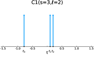
(a) Schematic representation of $\boldsymbol{x}$.

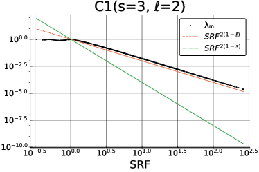
(b) The decay of $\lambda_{\min}$.

Figure 3.1: For different values of $\Delta,\Omega$ we plot the quantity $\lambda_{m}=\lambda_{\min}\left(\mathbf{G}\left(\boldsymbol{x},\Omega\right)\right)$ versus the super-resolution factor $\mathrm{SRF}=\frac{\pi}{\Delta\Omega}$. (a) $\boldsymbol{x}=\left(t_{1}=\Delta,\;t_{2}=2\Delta,\;t_{3}=-\frac{\pi}{4}\right)$ is a single cluster with $s=3$ and $\ell=2$. (b) The correct scaling is seen to be $\lambda_{m}\sim\left(\Delta\Omega\right)^{2\left(\ell-1\right)}$ rather than $\lambda_{m}\sim\left(\Delta\Omega\right)^{2\left(s-1\right)}$. See Section 5 for further details regarding the experimental setup. The relationship breaks when $\mathrm{SRF}\leq O(1)$, consistent with (2.6).

In this paper we bridge this theoretical gap. We consider the partially clustered regime where at most $2\leq\ell\leq s$ neighboring nodes can form a cluster (there can be several such clusters), with two additional parameters $\rho,\tau,$ controlling the distance between the clusters and the uniformity of the distribution of nodes within the clusters.

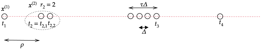
Figure 3.2: The schematic representation of a cluster configuration according to Definition 3.1. Here $s=8$ and $\ell=4$. Each node $t_{j}$ defines its “cluster” $\boldsymbol{x}^{(j)}$ of size $r_{j}\leq\ell$. $\rho$ is the minimal distance from any node $t_{j}$ to another node $y$ not in $\boldsymbol{x}^{(j)}$. The distance between any two nodes in $\boldsymbol{x}^{(j)}$ is between $\Delta$ and $\tau\Delta$.

Definition 3.1.

The node vector $\boldsymbol{x}=\left(t_{1},\dots,t_{s}\right)\subset(-\frac{\pi}{2},\frac{\pi}{2}]$ is said to form a $\left(\Delta,\rho,s,\ell,\tau\right)$-clustered configuration for some $\Delta>0$, $2\leq\ell\leq s$, $\ell-1\leq\tau<{\pi\over\Delta}$ and $\rho\geq 0$, if for each $t_{j}$, there exist at most $\ell$ distinct nodes

$$\boldsymbol{x}^{(j)}=\{t_{j,k}\}_{k=1,\dots,r_{j}}\subset\boldsymbol{x},\;1\leq r_{j}\leq\ell,\quad t_{j,1}\equiv t_{j},$$

such that the following conditions are satisfied:

1. For any $y\in\boldsymbol{x}^{(j)}\setminus\{t_{j}\}$, we have

   $$\Delta\leq\|y-t_{j}\|_{\mathbb{T}}\leq\tau\Delta.$$

2. For any $y\in\boldsymbol{x}\setminus\boldsymbol{x}^{(j)}$, we have

   $$\|y-t_{j}\|_{\mathbb{T}}\geq\rho.$$

The different parameters are illustrated in Figure 3.2.

Our main result is the following generalization of (2.7) for clustered configurations.

Theorem 3.2.

There exists a constant $\Cl{main-c-n}=\Cr{main-c-n}\left(s\right)$ such that for any $4\tau\Delta\leq\rho$, any $\boldsymbol{x}$ forming a $\left(\Delta,\rho,s,\ell,\tau\right)$-clustered configuration, and any $\Omega$ satisfying

$$\frac{4\pi s}{\rho}\leq\Omega\leq{\pi s\over{\tau\Delta}},$$ (3.1)

we have

$$\sigma_{\min}\left(\mathbf{V}_{N}\left(\boldsymbol{x},\Omega\right)\right) \geq\Cr{main-c-n}\cdot\left(\Delta\Omega\right)^{\ell-1},\qquad\text{ whenever }N>2s^{3}\left\lceil\frac{\Omega}{4s}\right\rceil;$$ (3.2)

$$\lambda_{\min}\left(\mathbf{G}\left(\boldsymbol{x},\Omega\right)\right) \geq\Cr{main-c-n}^{2}\cdot\left(\Delta\Omega\right)^{2\left(\ell-1\right)}.$$ (3.3)

The proof of Theorem 3.2 is presented in Subsection 4.3 below. It is based on the “decimation-and-blowup” technique, previously used in the context of super-resolution in [1, 2, 6, 7, 8] and references therein. In a nutshell, the main idea is to choose an appropriate “decimation” parameter $\lambda\approx\Omega$ such that the “inflated” nodes in the vector $\lambda\boldsymbol{x}$ (considered in the wrap-around sense) are separated by $\lambda\Delta\approx\Omega\Delta$ from its cluster neighbors, and by a constant from the other nodes. Then we fix sufficiently large $N$ and divide the $2N+1$ rows of $\mathbf{V}_{N}$ into groups of $s$ rows, separated by $\lambda N\over\Omega$. Each of the resulting square Vandermonde matrices can be explicitly estimated (the inverses have well-known behaviour), and has smallest singular value of the order ${1\over\sqrt{N}}\left(\Delta\Omega\right)^{\ell-1}$. The main technical part is to show that such $\lambda$ exists, and it is proved in Lemma 4.1 by a union bound argument, showing that the measure of all “bad” values of $\lambda$ (causing a collision of at least two nodes) is small. The condition on $N$ in (3.2) is obtained by accurate counting of how many such “bad” intervals exist.

Remark 3.3.

The condition $4\tau\Delta\leq\rho$ ensures that the range of admissible $\Omega$ is non-empty, and it will clearly be satisfied for all small enough $\Delta$ with all the rest of the parameters fixed.

Remark 3.4.

The same node vector $\boldsymbol{x}$ can be regarded as a clustered configuration with different choices of the parameters $\left(\ell,\rho,\tau\right)$. For example, the vector $\boldsymbol{x}$ from the beginning of this section (and also Figure 3.1) is both $\left(\Delta,{\pi\over 4}+\Delta,3,2,1\right)$-clustered and $\left(\Delta,\rho,3,3,{\pi\over{4\Delta}}+2\right)$-clustered, with any $\rho$. To obtain as tight a bound as possible, one should choose the minimal $\ell$ such that the condition (3.1) is satisfied for $\Omega$ within the range of interest. For instance, $\Omega$ might be too small if $\rho$ is small enough, however by choosing $\ell=s$ one is able to increase $\rho$ without bound. See Figure 5.3 for a numerical example.

Remark 3.5.

The constant $\Cr{main-c-n}$ is given explicitly in (4.16), and it decays in $s$ like $\sim s^{-2s}$. It is plausible that the best possible bound would scale like $c^{-\ell}$ for some absolute constant $c>1$, see also Remark 3.7 below.

Our next result is the analogue of (3.2) for the Vandermonde matrix $\mathbf{V}_{N}$ as in (2.1), albeit under an extra assumption that the nodes are restricted to the interval $\frac{1}{s^{2}}\left(-\frac{\pi}{2},\frac{\pi}{2}\right]$.

Corollary 3.6.

There exists a constant $\Cl{main-vand}=\Cr{main-vand}\left(s\right)$ such that for any $4\tau\Delta\leq\min\left({\rho},{1\over{s^{2}}}\right)$, any $\boldsymbol{\xi}=\left(\xi_{1},\dots,\xi_{s}\right)\subset\frac{1}{s^{2}}\left(-\frac{\pi}{2},\frac{\pi}{2}\right]$ forming a $\left(\Delta,\rho,s,\ell,\tau\right)$-clustered configuration, and any $N$ satisfying

$$\max\left(\frac{4\pi s}{\rho},4s^{3}\right)\leq N\leq{\pi s\over{\tau\Delta}},$$ (3.4)

we have

$$\sigma_{\min}\left(\mathbf{V}_{N}\left(\boldsymbol{\xi}\right)\right)\geq\Cr{main-vand}\cdot\left(N\Delta\right)^{\ell-1}.$$ (3.5)

Proof.

Let us choose $\widetilde{\Omega}:={N\over s^{2}}$ so that for all $j=1,\dots,s$ we have

$$\widetilde{t}_{j}:={N\xi_{j}\over\widetilde{\Omega}}\in\left(-{\pi\over 2},{\pi\over 2}\right].$$

Further define $\widetilde{\Delta}:=s^{2}\Delta$, and $\widetilde{\rho}:=s^{2}\rho$. We immediately obtain that the vector $\widetilde{\boldsymbol{x}}:=\left(\widetilde{t}_{1},\dots,\widetilde{t}_{s}\right)$ forms a $\left(\widetilde{\Delta},\tilde{\rho},s,\ell,\tau\right)$-clustered configuration according to Definition 3.1, and the rectangular Vandermonde matrix $\mathbf{V}_{N}\left(\boldsymbol{\xi}\right)$ in (2.1) is precisely $\mathbf{V}_{N}\left(\widetilde{\boldsymbol{x}},\widetilde{\Omega}\right)$. Clearly, $4\tau\widetilde{\Delta}\leq s^{2}\rho=\widetilde{\rho}$, and also

$$\widetilde{\Omega}s^{2}=N\geq 4s^{3}\Longrightarrow{\widetilde{\Omega}\over{4s}}\geq 1\Longrightarrow{2\widetilde{\Omega}\over{4s}}>\left\lceil{\widetilde{\Omega}\over{4s}}\right\rceil\Longrightarrow N=\widetilde{\Omega}s^{2}>2s^{3}\left\lceil{\widetilde{\Omega}\over{4s}}\right\rceil.$$ (3.6)

Using (3.4), we obtain precisely the conditions (3.1) with $\widetilde{\Omega},\widetilde{\rho}$ in place of $\Omega,\rho$ respectively. Therefore the conditions of Theorem 3.2 are satisfied for $\widetilde{\boldsymbol{x}},\widetilde{\Omega},\widetilde{\rho},\widetilde{\Delta},\tau$, and so (3.5) follows immediately from (3.6) and (3.2), with $\Cr{main-vand}=\Cr{main-c-n}$. ∎

Remark 3.7.

During the revision of the present paper, the authors of [26] (second version) investigated the question of bounding $\sigma_{\min}(\mathbf{V}_{N})$ under assumptions on node distribution which are similar to our clustering model (they are called “sparse clumps” in [26].) They also obtain the scaling $\left(N\Delta\right)^{\ell-1}$ for the smallest singular value. Comparing their results to Corollary 3.6 (see also Remark 4 in their paper), we note the following.

1. They do not have the requirement that the vector $\boldsymbol{\xi}$ should be restricted to a small interval.

2. Their bounds hold whenever $N\geq s^{2}$, while we require $N\geq 4s^{3}$.

3. Although their model is more general, their constants are more complicated. Nevertheless, the corresponding constant $\Cr{main-vand}$ scales as $\ell^{-\ell}$ which is better than our $s^{-2s}$.

4. Their equation (2.5) in Theorem 2 requires the product $\rho N$ to be at least $\ell^{5/2}{20s\over{\sqrt{N\Delta}}}$, which essentially forces a single cluster if $\Delta$ is very small (or, alternatively, prevents $\Delta$ to be too small for certain $s,\ell$) . In contrast, our equation (3.4) only requires $\rho N\geq 4\pi s$, and therefore doesn’t have these restrictions (although both conditions require $\rho$ to grow with $s$.)

Remark 3.8.

Continuing the above discussion, we would like to emphasize that Corollary 3.6 is derived by discretization of the continuous setting of Theorem 3.2, and therefore it is perhaps not surprising that the conditions for which the scaling holds are not optimal.

Returning back to Theorem 3.2, it turns out that the bound (3.3) is asymptotically optimal.

Theorem 3.9.

There exists an absolute constant $\eta\ll 1$ and a constant $\Cl{upper}=\Cr{upper}\left(\ell\right)$ such that for any $2\leq\ell\leq s$ and any $\Delta$ satisfying $\Delta<{\pi\over{2(\ell-1)}}$, there exists a $\left(\Delta,\rho^{\prime},s,\ell,\tau^{\prime}\right)$-clustered configuration $\boldsymbol{x}_{\min}$ with $s$ nodes and certain $\rho^{\prime},\tau^{\prime}$ depending only on $s,\ell$, for which

$$\lambda_{\min}\left(\mathbf{G}\left(\boldsymbol{x}_{\min},\Omega\right)\right)\leq\Cr{upper}\cdot\left(\Delta\Omega\right)^{2\left(\ell-1\right)},\qquad\Delta\Omega<\eta.$$

The proof of Theorem 3.9 is presented in Subsection 4.4.

Finally we conclude with the optimal scaling for the condition number of $\mathbf{V}_{N}=\mathbf{V}_{N}\left(\boldsymbol{x},\Omega\right)$, which is of interest to some applications.

Corollary 3.10.

Fix $s,\ell,\rho,\tau$ and $\Omega$. As $\Delta\to 0$ and $N\to\infty$, for any $\left(\Delta,\rho,s,\ell,\tau\right)$-clustered configuration $\boldsymbol{x}$, we have

$$\kappa\left(\mathbf{V}_{N}\left(\boldsymbol{x},\Omega\right)\right):=\frac{\sigma_{\max}(\mathbf{V}_{N})}{\sigma_{\min}(\mathbf{V}_{N})}\asymp\mathrm{SRF}^{\ell-1}.$$

Proof.

It is immediate that as $N\to\infty$, the largest singular value (the spectral norm) of $\mathbf{V}_{N}$ is bounded from above by a constant:

$$\sigma_{\max}(\mathbf{V}_{N})=\|\mathbf{V}_{N}\|_{2}\leq\sqrt{s{{2N+1}\over{2N}}}\leq\sqrt{2s},$$

while the lower bound can be obtained by

$$\sigma_{max}(\mathbf{V}_{N})=\sqrt{\lambda_{\max}(\mathbf{G}_{N})}\geq\sqrt{{1\over{2N}}\max_{t\in\mathbb{R}}\mathcal{D}_{N}\left(t\right)}>1.$$

Combining this with Theorem 3.2 and Theorem 3.9 finishes the proof. ∎

3.2 Stable super-resolution of point sources

The problem of (sparse) super-resolution is to recover discrete, point-like objects from their noisy and bandlimited spectral measurements. It arises in many fields such as frequency estimation, sampling theory, array processing, astronomical imaging, seismic imaging, nonuniform FFT, statistics, radar signal detection, error correction codes, and others [4, 12, 13, 16, 10, 20, 28, 25, 35]. Our main results have direct implications for the problem of super-resolution under sparsity constraints, in the so-called “on-grid” model.

Definition 3.11.

For $\Delta>0$, denote by ${\cal T}_{\Delta}$ the discrete grid

$${\cal T}_{\Delta}:=\left\{k\Delta,\;k=-\left\lfloor{\pi\over{2\Delta}}\right\rfloor,\dots,\left\lfloor{\pi\over{2\Delta}}\right\rfloor\right\}\subset\left[-{\pi\over 2},{\pi\over 2}\right].$$

Definition 3.12.

For $\Delta,\rho,s,\ell,\tau$ as in Definition 3.1, let ${\cal R}:={\cal R}\left(\Delta,\rho,s,\ell,\tau\right)$ be the set of point measures of the form $\mu=\sum_{j=1}^{s}a_{j}\delta_{t_{j}}$, where $t_{j}\in{\cal T}_{\Delta}$ for all $j=1,\dots,s$, $\delta_{t}$ is the Dirac measure supported on $t\in\mathbb{R}$, $a_{j}\in\mathbb{C}$, and the node vector $\left(t_{1},\dots,t_{s}\right)$ forms a $\left(\Delta,\rho,s,\ell,\tau\right)$-clustered configuration according to Definition 3.1.

Consider the problem of reconstructing $\mu\in{\cal R}$ from approximate spectral data $\widehat{\mu}\left(\omega\right)$ restricted to some interval $\omega\in\left[-\Omega,\Omega\right]$. Here the Fourier transform $\widehat{\mu}$ is defined as

$$\mu=\sum_{j=1}^{s}a_{j}\delta_{t_{j}}\Longrightarrow\widehat{\mu}\left(\omega\right)=\sum_{j=1}^{s}a_{j}\exp\left(\imath\omega t_{j}\right).$$

The measurement space $L_{2}\left(\left[-\Omega,\Omega\right]\right)$ contains complex-valued square-integrable functions supported on $\left[-\Omega,\Omega\right]$, with the norm

$$\|f\|^{2}_{2,\Omega}:={1\over{2\Omega}}\int_{-\Omega}^{\Omega}|f\left(\omega\right)|^{2}d\omega.$$ (3.7)

Proceeding as in [16, 15], we define the minimax error for this problem as follows.

Definition 3.13.

For ${\cal R}$ as above, $\varepsilon>0$ and $\Omega>0$, the minimax error ${\cal E}={\cal E}({\cal R},\Omega,\varepsilon)$ is the quantity

$${\cal E}:=\inf_{\widetilde{\mu}\left(\Phi_{\mu,e}\right)\in{\cal R}}\sup_{\mu\in{\cal R}}\sup_{e\in L_{2}\left(\left[-\Omega,\Omega\right]\right),\;\|e\|_{2,\Omega}\leq\varepsilon}\|\widetilde{\mu}-\mu\|_{2},$$ (3.8)

where

• $\Phi_{\mu,e}\in L_{2}\left(\left[-\Omega,\Omega\right]\right)$ is the measurement function given by

  $$\Phi_{\mu,e}(\omega)=\widehat{\mu}(\omega)+e(\omega);$$ (3.9)

• $\widetilde{\mu}$ is any deterministic mapping from $L_{2}\left(\left[-\Omega,\Omega\right]\right)$ to ${\cal R}$;

• for $\mu=\sum_{j=1}^{s}a_{j}\delta_{t_{j}}$, the norm $\|\mu\|_{2}$ is the discrete $\ell_{2}$ norm of the coefficient vector:

  $$\|\mu\|_{2}:=\left(\sum_{j=1}^{s}|a_{j}|^{2}\right)^{1\over 2}.$$

Using arguments very similar to [33, 16, 15, 26] and the novel bounds of Theorem 3.2 and Theorem 3.9, we obtain the optimal rate for the minimax error for clustered on-grid super-resolution.

Theorem 3.14.

Fix $s\geq 1,\;2\leq\ell\leq s,\;\varepsilon>0$. Put $\mathrm{SRF}:={\pi\over{\Delta\Omega}}$. Then the following hold.

1. For any $\rho\geq 0,\;\ell-1\leq\tau$ and $M\geq\pi$, there exists $\alpha\geq M$ such that for all sufficiently small $\Delta$ it holds that

   $${\cal E}\left({\cal R}\left(\Delta,\rho,s,\ell,\tau\right),\Omega,\varepsilon\right)\leq C_{s,\ell}\mathrm{SRF}^{2\ell-1}\varepsilon,\quad\mathrm{SRF}=\alpha,$$ (3.10)

   for some absolute constant $C_{s,\ell}$ depending only on $s$ and $\ell$.

2. There exists an absolute constant $\beta\gg 1$ and $\rho^{\prime},\tau^{\prime}$, depending only on $s,\ell$, such that for any $\Delta<{\pi\over{2(2\ell-1)}}$ it holds that

   $${\cal E}\left({\cal R}\left(\Delta,\rho^{\prime},s,\ell,\tau^{\prime}\right),\Omega,\varepsilon\right)\geq C_{\ell}\mathrm{SRF}^{2\ell-1}\varepsilon,\quad\mathrm{SRF}>\beta,$$ (3.11)

   for some absolute constant $C_{\ell}$ depending only on $\ell$.

For the proof, see Subsection 4.5 below. This result generalizes [15, 26] (where the scaling ${\cal E}\asymp\mathrm{SRF}^{2\ell-1}\varepsilon$ was derived for $\ell=s$), as well as [33] (where it was shown that for positive $a_{j}$ it holds that ${\cal E}\lessapprox\mathrm{SRF}^{2\ell}\varepsilon$, with a comparable definition of the Rayleigh regularity $\ell$).

A different but closely related setting was considered in the seminal paper [16], where the measure $\mu$ was assumed to have infinite number of spikes on a grid of size $\Delta$, with one spike per unit of time on average, but whose local complexity was constrained to have not more than $R$ spikes per any interval of length $R$ (such $R$ is called the “Rayleigh index”). It was shown in [16] that the minimax recovery rate for such measures scales like $\mathrm{SRF}^{\alpha}$ where $2R-1\leq\alpha\leq 2R+1$. Our partial cluster model can therefore be regarded as the finite-dimensional version of these “sparsely clumped” measures with finite Rayleigh index, showing the same scaling of the error – polynomial in $\mathrm{SRF}$ and exponential in the “local complexity” of the signal.

If the grid assumption is relaxed, then one might wish to measure the accuracy of recovery $\|\widetilde{\mu}-\mu\|$ by comparing the locations of the recovered signal $\widetilde{\mu}$ with the true ones $\{t_{j}\}$. In this case, there are additional considerations which are required to derive the minimax rate, and it is possible to do so under the partial clustering assumptions. See [1, 8] for details, where we prove that ${\cal E}\asymp\mathrm{SRF}^{2\ell-1}\Delta\varepsilon$ in this scenario, for uniform bound on the noise $\|e\|_{\infty}:=\sup_{|\omega|\leq\Omega}\left|e\left(\omega\right)\right|\leq\varepsilon\lessapprox\mathrm{SRF}^{1-2\ell}$. The extreme case $\ell=s$ has been treated recently in [6, 7].

In the case of well-separated spikes (i.e. clusters of size $\ell=1$), a recent line of work using $\ell_{1}$ minimization ([12, 11, 17, 14] and the great number of follow-up papers) has shown that the problem is stable and tractable.

Therefore, the partial clustering case is somewhat mid-way between the extremes $\ell=1$ and $\ell=s$, and while our results in this paper (and also in [8]) show that it is much more stable than in the unconstrained sparse case, it is an intriguing open question whether provably tractable solution algorithms exist.

Several candidate algorithms for sparse super-resolution are well-known – MUSIC, ESPRIT/matrix pencil, and variants; these have roots in parametric spectral estimation [42]. In recent years, the super-resolution properties of these algorithms are a subject of ongoing interest, see e.g. [18, 29, 38, 26, 27] and references therein. Smallest singular values of the partial Fourier matrices $\mathbf{V}_{N}$, for finite $N$, play a major role in these works, and therefore we hope that our results and techniques may be extended to analyze these algorithms as well.

4 Proofs

4.1 Blowup

Here we introduce the uniform blowup of a node vector $\boldsymbol{x}=\left(t_{1},\dots,t_{s}\right)$ by a positive parameter $\lambda$, and study the effect of such a blowup mapping on the minimal wrap-around distance between the mapped nodes.

Lemma 4.1.

Let $\boldsymbol{x}$ form a $\left(\Delta,\rho,s,\ell,\tau\right)$ cluster, and suppose that $\frac{4\pi s}{\rho}\leq\Omega\leq{\pi s\over{\tau\Delta}}$. Then, for any $0\leq\xi\leq 1$ there exists a set $I\subset\left[{\Omega\over 2s},{\Omega\over s}\right]$ of total measure ${\Omega\over 2s}\xi$ such that for every $\lambda\in I$ the following holds for every $t_{j}\in\boldsymbol{x}$:

$$\|\lambda y-\lambda t_{j}\|_{\mathbb{T}} \geq\lambda\Delta\geq{\Delta\Omega\over{2s}}, \forall y\in\boldsymbol{x}^{(j)}\setminus\{t_{j}\};$$ (4.1)

$$\|\lambda y-\lambda t_{j}\|_{\mathbb{T}} \geq\frac{1-\xi}{s^{2}}\pi, \forall y\in\boldsymbol{x}\setminus\boldsymbol{x}^{(j)}.$$ (4.2)

Furthermore, the set $I^{c}:=\left[{\Omega\over{2s}},{\Omega\over s}\right]\setminus I$ is a union of at most ${s^{2}\over 2}\left\lceil{\Omega\over{4s}}\right\rceil$ intervals.

Proof.

We begin with (4.1). Let $\lambda\in\left[{\Omega\over 2s},{\Omega\over s}\right]$, then $\lambda\tau\Delta\leq\pi$ and since $\|t_{j}-y\|_{\mathbb{T}}\leq\tau\Delta$ we immediately conclude that

$$\|\lambda t_{j}-\lambda y\|_{\mathbb{T}}=\lambda\|t_{j}-y\|_{\mathbb{T}}\geq\lambda\Delta.$$

To show (4.2), let $\nu$ be the uniform probability measure on $\left[{\Omega\over 2s},{\Omega\over s}\right]$. Let $t_{j}\in\boldsymbol{x}$ and $y\in\boldsymbol{x}\setminus\boldsymbol{x}^{(j)}$ be fixed and put $\delta:=\|y-t_{j}\|_{\mathbb{T}}$. For $\lambda\in\left[{\Omega\over 2s},{\Omega\over s}\right]$, let $\gamma(\lambda)=\gamma^{(t_{j},y)}(\lambda)$ be the random variable on $\nu$, defined by

$$\gamma^{(t_{j},y)}(\lambda):=\|\lambda t_{j}-\lambda y\|_{\mathbb{T}}.$$

We now show that for any $0\leq\alpha\leq 1$

$$\nu\left\{\gamma\left(\lambda\right)\leq\alpha\pi\right\}\leq 2\alpha.$$ (4.3)

Since $\delta\geq\rho\geq{4\pi s\over\Omega}$, we can write ${\Omega\over{2s}}={2\pi\over\delta}\left(n+\zeta\right)$ where $n\geq 1$ is an integer and $0\leq\zeta<1$. We break up the probability (4.3) as follows:

$$\begin{split}\nu\left\{\gamma\left(\lambda\right)\leq\alpha\pi\right\}&=\sum_{k=1}^{n}\nu\left\{\gamma\left(\lambda\right)\leq\alpha\pi\Biggl{|}\lambda-{\Omega\over{2s}}\in{2\pi\over\delta}\left[k-1,k\right]\right\}\nu\left\{\lambda-{\Omega\over{2s}}\in{2\pi\over\delta}\left[k-1,k\right]\right\}\\ &\qquad+\nu\left\{\gamma\left(\lambda\right)\leq\alpha\pi\Biggl{|}\lambda-{\Omega\over{2s}}\in{2\pi\over\delta}\left[n,n+\zeta\right]\right\}\nu\left\{\lambda-{\Omega\over{2s}}\in{2\pi\over\delta}\left[n,n+\zeta\right]\right\}.\end{split}$$ (4.4)

Now, consider the number $a=y-t_{j}$. As $\lambda$ varies between ${\Omega\over{2s}}+{2(k-1)\pi\over\delta}$ and ${\Omega\over{2s}}+{2k\pi\over\delta}$, the number $\exp(\imath\lambda a)$ traverses the unit circle exactly once, and therefore the variable $\gamma(\lambda)$ traverses the interval $[0,\alpha\pi]$ exactly twice. Consequently,

$$\nu\left\{\gamma\left(\lambda\right)\leq\alpha\pi\Biggl{|}\lambda-{\Omega\over{2s}}\in{2\pi\over\delta}\left[k-1,k\right]\right\}=\frac{2\alpha\pi}{2\pi}=\alpha.$$

Similarly, when $\lambda$ varies between ${\Omega\over{2s}}+{2\pi n\over\delta}$ and ${\Omega\over{2s}}+{2\pi(n+\zeta)\over\delta}$, we have

$$\nu\left\{\gamma\left(\lambda\right)\leq\alpha\pi\Biggl{|}\lambda-{\Omega\over{2s}}\in{2\pi\over\delta}\left[n,n+\zeta\right]\right\}\leq\frac{2\alpha\pi}{2\pi\zeta}\leq{\alpha\over\zeta}.$$

Overall,

$$\nu\left\{\gamma\left(\lambda\right)\leq\alpha\pi\right\}\leq\alpha{n\over{n+\zeta}}+{\alpha\over\zeta}\frac{\zeta}{n+\zeta}=\alpha{n+1\over{n+\zeta}}\leq 2\alpha,$$

proving (4.3).

It is clear from the above that $\left\{\lambda:\gamma\left(\lambda\right)\leq\alpha\pi\right\}$ is a union of intervals, each of length $2\alpha\pi$, repeating with the period of $\frac{2\pi}{\delta}$. Consequently the set $\left\{\lambda\in\left[{\Omega\over 2s},{\Omega\over s}\right]:\gamma\left(\lambda\right)\leq\alpha\pi\right\}$ is a union of at most $\left\lceil\frac{\Omega}{2s}\frac{\delta}{2\pi}\right\rceil$ intervals. Since $\delta\leq\pi$ we have $\left\lceil\frac{\Omega}{2s}\frac{\delta}{2\pi}\right\rceil\leq\left\lceil{\Omega\over{4s}}\right\rceil$, and so the set $\left\{\lambda\in\left[{\Omega\over 2s},{\Omega\over s}\right]:\gamma\left(\lambda\right)\leq\alpha\pi\right\}$ is a union of at most $\left\lceil{\Omega\over{4s}}\right\rceil$ intervals.

Now we put $\alpha_{0}={1-\xi\over s^{2}}$ and apply (4.3) for every pair $\left(t_{j},y\right)$ where $j=1,\dots,s$ and $y\in\boldsymbol{x}\setminus\boldsymbol{x}^{(j)}$. Denote

$$J:=\bigcup_{t_{j},y\in\boldsymbol{x}\setminus\boldsymbol{x}^{(j)}}\left\{\lambda\in\left[{\Omega\over 2s},{\Omega\over s}\right]:\gamma^{(t_{j},y)}(\lambda)\leq\alpha_{0}\pi\right\},$$

then by the union bound we obtain

$$\nu\left(J\right)\leq\sum_{t_{j},y}2\alpha_{0}=2{s\choose 2}{1-\xi\over s^{2}}<1-\xi.$$ (4.5)

Fixing $I$ as the complement of the above set, $I=\left[{\Omega\over 2s},{\Omega\over s}\right]\setminus J$, we have that $I$ is of total measure greater or equal to $\xi{\Omega\over{2s}}$, and for every $\lambda\in I$ the estimate (4.2) holds. Clearly $J$ is a union of at most ${s^{2}\over 2}\left\lceil{\Omega\over{4s}}\right\rceil$ intervals. ∎

Fix $\xi={1\over 2}$ and consider the set $I$ given by Lemma 4.1. Let us also fix a finite and positive integer $N$, and consider the set of $2N+1$ equispaced points in $\left[-\Omega,\Omega\right]$:

$$P_{N}:=\left\{k{\Omega\over N}\right\}_{k=-N,\dots,N}.$$

Proposition 4.2.

If $N>2s^{3}\left\lceil{\Omega\over{4s}}\right\rceil$, then $P_{N}\cap I\neq\emptyset$.

Proof.

By Lemma 4.1, the set $I^{c}$ consists of $K\leq{s^{2}\over 2}\left\lceil{\Omega\over{4s}}\right\rceil$ intervals, and by (4.5) the total length of $I^{c}$ is at most ${\Omega\over{4s}}$. Denote the lengths of those intervals by $d_{1},\dots,d_{K}$. The distance between neighboring points in $P_{N}$ is ${\Omega\over N}$, and therefore each interval contains at most ${d_{j}N\over\Omega}+1$ points. Overall, the interval $I^{c}$ contains at most

$$\sum_{j=1}^{K}\left({d_{j}N\over\Omega}+1\right)\leq{\Omega\over{4s}}{N\over\Omega}+K$$

points from $P_{N}$, and since the total number of points in $\left[{\Omega\over{2s}},{\Omega\over s}\right]$ is at least ${N\over{2s}}$, we have

$$\left|P_{N}\cap I\right|\geq{N\over{2s}}-{N\over{4s}}-K\geq{N\over{4s}}-{s^{2}\over 2}\left\lceil{\Omega\over{4s}}\right\rceil>0.$$

∎

4.2 Square Vandermonde matrices

Let $\boldsymbol{\xi}=\left(\xi_{1},\dots,\xi_{s}\right)$ be a vector of $s$ pairwise distinct complex numbers. Consider the square Vandermonde matrix

$$\mathbf{V}(\boldsymbol{\xi}):=\begin{bmatrix}1&1&\dots&1\\ \xi_{1}&\xi_{2}&\dots&\xi_{s}\\ \xi_{1}^{2}&\xi_{2}^{2}&\dots&\xi_{s}^{2}\\ \vdots&\vdots&\ddots&\vdots\\ \xi_{1}^{s-1}&\xi_{2}^{s-1}&\dots&\xi_{s}^{s-1}\end{bmatrix}.$$ (4.6)

Theorem 4.3 (Gautschi, [21]).

For a matrix $A=(a_{i,j})\in\mathbb{C}^{m\times n}$, let $\|A\|_{\infty}$ denote the $\ell_{\infty}$ induced matrix norm

$$\|A\|_{\infty}:=\max_{1\leq i\leq m}\sum_{1\leq j\leq n}|a_{i,j}|.$$

Then we have

$$\|\mathbf{V}^{-1}\left(\boldsymbol{\xi}\right)\|_{\infty}\leq\max_{1\leq i\leq s}\prod_{j\neq i}\frac{1+|\xi_{j}|}{|\xi_{j}-\xi_{i}|}.$$ (4.7)

Proposition 4.4.

Suppose that $\boldsymbol{\xi}=\left(\xi_{1},\dots,\xi_{s}\right)$ is a vector of pairwise distinct complex numbers with $|\xi_{j}|=1$, $j=1,\dots,s$, and let $r\in\mathbb{R}$ be arbitrary. Let

$$\mathbf{V}\left(\boldsymbol{\xi},r\right):=\begin{bmatrix}\xi_{1}^{r}&\xi_{2}^{r}&\dots&\xi_{s}^{r}\\ \xi_{1}^{r+1}&\xi_{2}^{r+1}&\dots&\xi_{s}^{r+1}\\ \xi_{1}^{r+2}&\xi_{2}^{r+2}&\dots&\xi_{s}^{r+2}\\ \vdots&\vdots&\ddots&\vdots\\ \xi_{1}^{r+s-1}&\xi_{2}^{r+s-1}&\dots&\xi_{s}^{r+s-1}\end{bmatrix}.$$ (4.8)

For $1\leq j<k\leq s$, denote by $\delta_{j,k}$ the angular distance between $\xi_{j}$ and $\xi_{k}$:

$$\delta_{j,k}:=\left|\operatorname{Arg}\left({\xi_{j}\over\xi_{k}}\right)\right|=\bigl{|}\operatorname{Arg}(\xi_{j})-\operatorname{Arg}(\xi_{k})\mod(-\pi,\pi]\bigr{|}.$$

Then

$$\sigma_{\min}\left(\mathbf{V}\left(\boldsymbol{\xi},r\right)\right)\geq{\pi^{1-s}\over\sqrt{s}}\min_{1\leq j\leq s}\prod_{k\neq j}\delta_{j,k}.$$ (4.9)

Proof.

Clearly, the matrix $\mathbf{V}\left(\boldsymbol{\xi},r\right)$ can be factorized as

$$\mathbf{V}\left(\boldsymbol{\xi},r\right)=\mathbf{V}\left(\boldsymbol{\xi},0\right)\times\operatorname{diag}\left\{\xi_{1}^{r},\dots,\xi_{s}^{r}\right\}.$$

Since $\mathbf{V}\left(\boldsymbol{\xi},0\right)=\mathbf{V}\left(\boldsymbol{\xi}\right)$ as in (4.6), using (4.7) we immediately have

$$\|\mathbf{V}^{-1}\left(\boldsymbol{\xi},r\right)\|_{\infty}\leq 2^{s-1}\max_{1\leq j\leq s}\prod_{k\neq j}|\xi_{j}-\xi_{k}|^{-1}.$$ (4.10)

For any $|\theta|\leq{\pi\over 2}$ we have

$${2\over\pi}\left|\theta\right|\leq\sin\left|\theta\right|\leq\left|\theta\right|,$$

and since for any $\xi_{j}\neq\xi_{k}$

$$\left|\xi_{j}-\xi_{k}\right|=\left|1-{\xi_{j}\over\xi_{k}}\right|=2\sin\left|{1\over 2}\operatorname{Arg}{\xi_{j}\over\xi_{k}}\right|=2\sin\left|{\delta_{j,k}\over 2}\right|,$$

we therefore obtain

$${2\over\pi}\delta_{j,k}\leq\left|\xi_{j}-\xi_{k}\right|\leq\delta_{j,k}.$$ (4.11)

Plugging (4.11) into (4.10) we have

$$\sigma_{\max}\left(\mathbf{V}^{-1}\left(\boldsymbol{\xi},r\right)\right)\leq\sqrt{s}\|\mathbf{V}^{-1}\left(\boldsymbol{\xi},r\right)\|_{\infty}\leq\sqrt{s}\pi^{s-1}\max_{1\leq j\leq s}\prod_{k\neq j}\delta_{j,k}^{-1},$$

which is precisely (4.9). ∎

4.3 Proof of Theorem 3.2

We shall bound $\sigma_{\min}\left(\mathbf{V}_{N}\left(\boldsymbol{x},\Omega\right)\right)$ defined as in (2.2) for sufficiently large $N$. For any subset $R\subset\left\{-N,\ldots,N\right\}$ let $\mathbf{V}_{N,R}$, be the submatrix of $\mathbf{V}_{N}$ containing only the rows in $R$. By the Rayleigh characterization of singular values, it is immediately obvious that if $\left\{-N,\ldots,N\right\}=R_{1}\cup\dots\cup R_{P}$ is any partition of the rows of $\mathbf{V}_{N}$ then

$$\sigma^{2}_{\min}(\mathbf{V}_{N})\geq\sum_{n=1}^{P}\sigma^{2}_{\min}(\mathbf{V}_{N,R_{n}}).$$ (4.12)

Let $I$ be the set from Lemma 4.1 for $\xi={1\over 2}$. By Proposition 4.2 we have that for all $N>2s^{3}\left\lceil\frac{\Omega}{4s}\right\rceil$, $I$ will contain a rational multiple of $\Omega$ of the form $\lambda_{N}={\Omega\over N}m$ for some $m\in\mathbb{N}$.

Consider the ”new” nodes

$$u_{j,N}:=t_{j}{\Omega\over N}m=\lambda_{N}t_{j},\hskip 20.00003ptj=1,\dots,s.$$ (4.13)

Since $\lambda_{N}\in I$, we conclude by Lemma 4.1 that for every $j=1,\dots,s$

$$\|u_{j,N}-u_{k,N}\|_{\mathbb{T}} \geq{1\over 2s}(\Delta\Omega), \forall t_{k}\in\boldsymbol{x}^{(j)}\setminus\{t_{j}\};$$ (4.14)

$$\|u_{j,N}-u_{k,N}\|_{\mathbb{T}} \geq{\pi\over 2s^{2}}, \forall t_{k}\in\boldsymbol{x}\setminus\boldsymbol{x}^{(j)}.$$ (4.15)

Since $\lambda_{N}\leq{\Omega\over s}$ it follows that $ms\leq N$. Now consider the particular interleaving partition of the rows $\left\{-N,\ldots,N\right\}$ by blocks $R_{-m},\dots,R_{-1},\allowbreak R_{0},R_{1},\ldots,R_{m}$ of $s$ rows each, separated by $m-1$ rows between them (some rows might be left out):

$$R_{0} =\left\{0,m,\dots,(s-1)m\right\},$$

$$R_{1} =\left\{1,m+1,\dots,(s-1)m+1\right\},$$

$$R_{-1} =\left\{-1,-m-1,\dots,-(s-1)m-1\right\},$$

$$\dots$$

$$R_{m-1} =\left\{m-1,2m-1,\dots,sm-1\right\},$$

$$R_{-m+1} =\left\{-m+1,-2m+1,\dots,-sm+1\right\}.$$

For $n=-m+1,\ldots,m-1$, each $\mathbf{V}_{N,R_{n}}$ is a square Vandermonde-type matrix as in (4.8),

$$\mathbf{V}_{N,R_{n}}={1\over\sqrt{2N}}\mathbf{V}\left(\boldsymbol{\xi},n\right),$$

with node vector

$$\boldsymbol{\xi}=\left\{e^{\imath u_{j,N}}\right\}_{j=1}^{s},$$

where $u_{j,N}$ are given by (4.13). We apply Proposition 4.4 with the crude bound obtained from (4.14) and (4.15) above:

$$\min_{1\leq j\leq s}\prod_{k\neq j}\delta_{j,k}\geq{1\over 2^{s-1}s^{2s-2}}\left(\Delta\Omega\right)^{\ell-1}$$

and obtain

$$\sigma_{\min}\left(\mathbf{V}_{N,R_{n}}\right)\geq{\Cl{aux1}(s)\over\sqrt{2N}}\left(\Delta\Omega\right)^{\ell-1},\qquad\Cr{aux1}(s):=\frac{1}{(2\pi)^{s-1}s^{2s-2}\sqrt{s}}.$$

Now we use (4.12) to aggregate the bounds on $\sigma_{\min}$ for each square matrix $\mathbf{V}_{N,R_{n}}$ and obtain

$$\lambda_{\min}\left(\mathbf{V}_{N}^{H}\mathbf{V}_{N}\right)=\sigma^{2}_{\min}\left(\mathbf{V}_{N}\right)\geq(2m-1)\frac{\Cr{aux1}^{2}}{2N}\left(\Delta\Omega\right)^{2\left(\ell-1\right)}.$$

Since $m=\frac{\lambda_{N}N}{\Omega}\geq\frac{\Omega N}{2s\Omega}=\frac{N}{2s}$ and since by assumption $N>2s^{3}$, we have that ${2m-1\over{2N}}\geq\frac{1}{4s}$ and so

$$\sigma^{2}_{\min}\left(\mathbf{V}_{N}\right)\geq\frac{\Cr{aux1}^{2}}{4s}\left(\Delta\Omega\right)^{2\left(\ell-1\right)}.$$

This proves (3.2) and (3.3) with

$$\Cr{main-c-n}(s):=\frac{1}{2(2\pi)^{s-1}s^{2s-1}}.$$ (4.16)

4.4 Proof of Theorem 3.9

Let $\ell,s,\Delta,\Omega$ be fixed, with $\Delta\Omega<\eta$, where $\eta$ will be specified during the proof below, and $\Delta<{\pi\over{2\left(\ell-1\right)}}$. We shall exhibit a $\left(\Delta,\rho^{\prime},s,\ell,\tau^{\prime}\right)$-clustered configuration $\boldsymbol{x}_{\min}$ with certain $\rho^{\prime},\tau^{\prime}$, such that

$$\lambda_{\min}\left(\mathbf{G}\left(\boldsymbol{x}_{\min},\Omega\right)\right)\leq\Cr{upper}\cdot\left(\Delta\Omega\right)^{2\left(\ell-1\right)},$$ (4.17)

for some constant $\Cr{upper}=\Cr{upper}\left(\ell\right)$.

Define $\boldsymbol{x}_{\ell,\Delta}=\{t_{1},\dots,t_{\ell}\}$ to be the vector of $\ell$ equispaced nodes separated by $\Delta$, i.e. $t_{j}=j\Delta,\;j=1,\dots,\ell$. Let $\mathbf{G}^{(\ell,\ell)}=\mathbf{G}\left(\boldsymbol{x}_{\ell,\Delta},\Omega\right)$ be the corresponding $\ell\times\ell$ prolate matrix.

Proposition 4.5.

There exists an absolute constant $0<\eta_{1}\ll 1$ and $\Cl{slepian-const}=\Cr{slepian-const}\left(\ell\right)$ such that whenever $\Omega\Delta\leq\eta_{1}$, we have

$$\lambda_{\min}\left(\mathbf{G}^{(\ell,\ell)}\right)\leq\Cr{slepian-const}\cdot\left(\Omega\Delta\right)^{2\left(\ell-1\right)}.$$ (4.18)

Proof.

By Slepian’s results [40] elaborated in Section 2, there exists a constant $\eta^{\prime}\ll 1$ for which (2.5) holds for all $s$, in particular for $s=\ell$, whenever $W\leq\eta^{\prime}$, i.e. whenever $\Omega\Delta\leq\eta_{1}:=2\pi\eta^{\prime}$. ∎

We define $\boldsymbol{x}_{\min}$ to be the extension of $\boldsymbol{x}_{\ell,\Delta}$ such that the remaining $s-\ell$ nodes are maximally equally spaced between $-{\pi\over 2}$ and $0$, not including the endpoints. Under the assumptions on $s,\ell,\Delta$ specified in Theorem 3.9, it is easy to check that the nodes $t_{1},\dots,t_{\ell}$ are between $0$ and ${\pi\over 2}$, while the remaining nodes are separated at least by

$$\rho^{\prime}:={\pi\over{2\left(s-\ell+1\right)}}.$$ (4.19)

Therefore, $\boldsymbol{x}_{\min}$ is a particular $\left(\Delta,\rho^{\prime},s,\ell,\tau^{\prime}\right)$-clustered configuration according to Definition 3.1, with $\rho^{\prime}$ given by (4.19) and $\tau^{\prime}:=\ell-1$.

It is clear that $\mathbf{G}^{\left(\ell,\ell\right)}$ is a principal submatrix of $\mathbf{G}\left(\boldsymbol{x}_{\min},\Omega\right)$, and therefore we can apply the interlacing theorem for eigenvalues of partitioned Hermitian matrices [22, Theorem 4.3.28]. Together with (4.18), this concludes the proof of (4.17) and of Theorem 3.9 with $\Cr{upper}=\Cr{slepian-const}$ and $\eta=\eta_{1}$. ∎

4.5 Proof of Theorem 3.14

By the definition of the matrix $\mathbf{G}$ and (3.7), we immediately obtain the following fact.

Proposition 4.6.

For $\mu=\sum_{j=1}^{s}a_{j}\delta_{t_{j}}\in{\cal R}$, denote $\boldsymbol{x}=\boldsymbol{x}_{\mu}:=\operatorname{supp}\mu=\left(t_{1},\dots,t_{s}\right)\in\mathbb{R}^{s}$ and $\boldsymbol{c}=\boldsymbol{c}_{\mu}:=\left(a_{1},\dots,a_{s}\right)\in\mathbb{C}^{s}$. Then we have

$$\|\widehat{\mu}\|_{2,\Omega}^{2}=\boldsymbol{c}^{*}\mathbf{G}\left(\boldsymbol{x},\Omega\right)\boldsymbol{c}.$$

The next result shows that for any two measures with $s$ nodes and clusters of size $\ell$, their difference has clusters of size at most $2\ell$, provided that the grid size is small enough. Note that it may happen that some nodes are in the support of both measures, in which case the difference measure will have less than $2s$ nodes, and the largest cluster may be of size strictly smaller than $2\ell$.

Lemma 4.7.

Fix $s,\ell,\rho,\tau$, and let there be given $K\geq 2$. Then there exists $\Delta_{0}$ such that for all $\Delta\leq\Delta_{0}$ the following holds: for any $\mu_{1},\mu_{2}\in{\cal R}\left(\Delta,\rho,s,\ell,\tau\right)$ we have

$$\mu_{1}-\mu_{2}\in{\cal R}\left(\Delta,\rho^{\prime},s^{\prime},\ell^{\prime},\tau^{\prime}\right)$$

for some $\ell^{\prime}\leq 2\ell,\;s^{\prime}\leq 2s$, some $\rho^{\prime},\tau^{\prime}$ satisfying $\rho^{\prime}=K\tau^{\prime}\Delta$ and $\tau^{\prime}\geq 1$.

Proof.

Let $\Delta\leq\Delta_{0}$ be given (with $\Delta_{0}$ to be determined below), and put $\rho_{0}:=\tau\Delta$.

Consider the intervals $I_{0},I_{1},\dots,I_{2s+2}$ (see Figure 4.1):

$$I_{0} =\left[0,\rho_{0}\right],$$

$$I_{1} =\left[\rho_{0},K\rho_{0}\right],$$

$$I_{2} =\left[K\rho_{0},K^{2}\rho_{0}\right],$$

$$\dots$$

such that the length $a_{j}$ of each $I_{j}$ is

$$a_{0} =|I_{0}|=\rho_{0};$$

$$a_{j} =|I_{j}|=(K-1)\cdot K^{j-1}\rho_{0},\quad j\geq 1.$$

One can verify that

$$a_{n} =(K-1)\sum_{j=0}^{n-1}a_{j},\quad n\geq 1;$$

$$\sum_{j=0}^{n}a_{j} =K^{n}\rho_{0},\quad n\geq 0.$$

The overall length of the $2s+3$ intervals is therefore $K^{2s+2}\rho_{0}$. From now on we assume that this quantity is at most ${\rho\over 2}$, which in particular means that $\Delta\leq\Delta_{0}:={\rho\over{2\tau K^{2s+2}}}$.

For each $t_{j}\in\operatorname{supp}\mu_{1}$, consider the following sets of distances:

$${\cal R}_{j} :=\{\|y-t_{j}\|_{\mathbb{T}}:\;y\in\operatorname{supp}\mu_{1}\}\cap\left[0,{\rho\over 2}\right],$$

$${\cal S}_{j} :=\{\|y-t_{j}\|_{\mathbb{T}}:\;y\in\operatorname{supp}\mu_{2}\}\cap\left[0,{\rho\over 2}\right].$$

It is obvious that

$$\left(\bigcup_{j=1}^{s}{\cal R}_{j}\right)\cap\left(\bigcup_{j=2}^{2s+2}I_{j}\right)=\emptyset.$$

Now, since $\mu_{2}\in{\cal R}$, each one of the sets ${\cal S}_{1},\dots,{\cal S}_{s}$ intersects at most two of the intervals $I_{2},\dots,\allowbreak I_{2s+2}$. Therefore, by the pigeonhole’s principle (Dirichlet’s principle), there exists an index $C\in\left\{2,\dots,2s+2\right\}$ such that

$$I_{C}\bigcap\left(\bigcup_{j=1}^{s}{\cal S}_{j}\right)=\emptyset.$$

Clearly we also have $I_{C}\bigcap\left(\bigcup_{j=1}^{s}{\cal R}_{j}\right)=\emptyset$. Put $I_{C}=[a,b]$. The proof is finished by taking $\tau^{\prime}:={a\over\Delta}\geq{K\rho_{0}\over\Delta}=\tau\geq 1$ and $\rho^{\prime}:=b=Ka=K\tau^{\prime}\Delta$. ∎

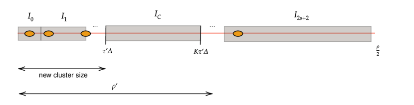
Figure 4.1: Merging $\mu_{1}$ and $\mu_{2}$ - see Lemma 4.7. The orange circles are the sets ${\cal S}_{j}$, $j=1,\dots,s$.

Proof of upper bound.

Let $s,\ell,\tau,\rho$ and $\varepsilon$ be fixed. Put $K:=8sM$ and let $\Delta_{0}$ be as specified in Lemma 4.7. Let $\Delta\leq\Delta_{0}$, and put ${\cal R}={\cal R}\left(\Delta,\rho,s,\ell,\tau\right)$ as in Definition 3.12.

Since the set ${\cal R}$ is finite, it is clearly possible to enumerate all its elements. To prove the upper bound for the minimax error rate ${\cal E}$, consider the following estimator (clearly realizable, but computationally intractable) function $\widetilde{\mu}_{0}=\mu_{{\cal R},\Omega,\varepsilon}:L_{2}\left([-\Omega,\Omega]\right)\to{\cal R}$:

$$\widetilde{\mu}_{0}\left(\Phi\right):=\left\{\textrm{the first }\mu\in{\cal R}\quad\textit{ subject to }\|\Phi-\widehat{\mu}\|_{2,\Omega}\leq\varepsilon\right\}.$$

Given $\mu\in{\cal R}$ and $e\in L_{2}\left([-\Omega,\Omega]\right)$ with $\|e\|_{2,\Omega}\leq\varepsilon$, let $\widetilde{\mu}_{0}=\widetilde{\mu}_{0}\left(\Phi_{\mu,e}\right)$ where $\Phi_{\mu,e}$ is given by (3.9). Then, since $\|\Phi_{\mu,e}-\widehat{\mu}\|_{2,\Omega}=\|e\|_{2,\Omega}\leq\varepsilon$ and also by the definition of $\widetilde{\mu}_{0}$, we have

$$\|\widehat{\widetilde{\mu}}_{0}-\widehat{\mu}\|_{2,\Omega}\leq 2\varepsilon.$$

Denote $\mu_{2}:=\widetilde{\mu}_{0}-\mu$. By Lemma 4.7, we get that $\mu_{2}\in{\cal R}\left(\Delta,\rho^{\prime},s^{\prime},\ell^{\prime},\tau^{\prime}\right)$ where $s^{\prime}\leq 2s$, $\ell^{\prime}\leq 2\ell$, $\tau^{\prime}\geq 1$ and $\rho^{\prime}=8sM\tau^{\prime}\Delta$. In particular, $\rho^{\prime}>4\tau^{\prime}\Delta$, and therefore by applying Theorem 3.2 we obtain that for all $\Omega$ satisfying

$${\pi s^{\prime}\over{2sM\tau^{\prime}\Delta}}={4\pi s^{\prime}\over{\rho^{\prime}}}\leq\Omega\leq{{\pi s^{\prime}}\over{\tau^{\prime}\Delta}},$$

it holds that

$$\sqrt{\lambda_{\min}\left(\mathbf{G}\left(\operatorname{supp}\mu_{2},\Omega\right)\right)}\geq\Cr{main-c-n}(s^{\prime})\left(\Omega\Delta\right)^{\ell^{\prime}-1}.$$

In particular, for ${\pi\over{\Omega\Delta}}:=\alpha=M\tau^{\prime}{2s\over s^{\prime}}\geq M$, we have, using the above and Proposition 4.6, that

$$2\varepsilon\geq\|\widehat{\mu}_{2}\|_{2,\Omega} \geq\sqrt{\lambda_{\min}\left(\mathbf{G}\left(\operatorname{supp}\mu_{2},\Omega\right)\right)}\|\mu_{2}\|_{2}$$

$$\geq\Cr{main-c-n}(s^{\prime})\left(\Omega\Delta\right)^{\ell^{\prime}-1}\|\mu_{2}\|_{2}$$

$$\geq\Cr{main-c-n}(2s)\left(\Omega\Delta\right)^{2\ell-1}\|\mu_{2}\|_{2}$$

(here we also used that the constant $\Cr{main-c-n}(s)$ is decreasing with $s$ and $\Delta\Omega<1$). This in turn proves that ${\cal E}\leq{2\over{\Cr{main-c-n}(2s)\pi^{2\ell-1}}}\mathrm{SRF}^{2\ell-1}\varepsilon$. ∎

Proof of the lower bound.

Let $\eta$ be the constant from Theorem 3.9, and put $\beta:={\pi\over\eta}$. Now suppose that $\alpha:=\mathrm{SRF}>\beta$, that is, ${\Omega\Delta}<\eta$. Applying Theorem 3.9 with $2s,2\ell$ we obtain $\rho^{\prime},\tau^{\prime}$ and the minimal configuration $\boldsymbol{x}_{\alpha}$. Let $\boldsymbol{c}_{\alpha}\in\mathbb{C}^{2s}$ denote the corresponding minimal eigenvector of $\mathbf{G}\left(\boldsymbol{x}_{\alpha},\Omega\right)$, with the normalization

$$\|\boldsymbol{c}_{\alpha}\|_{2}^{2}=\frac{\varepsilon^{2}}{\Cr{upper}\alpha^{2(2\ell-1)}}.$$ (4.20)

Let $\mu$ be the measure defined by $\boldsymbol{x}_{\alpha},\boldsymbol{c}_{\alpha}$, which therefore satisfies $\mu\in{\cal R}\left(\Delta,\rho^{\prime},2s,2\ell,\tau^{\prime}\right)$. By Proposition 4.6, (4.20) and Theorem 3.9 we have

$$\|\widehat{\mu}\|_{2,\Omega}^{2}=\lambda_{\min}\left(\mathbf{G}\left(\boldsymbol{x}_{\alpha},\Omega\right)\right)\|\boldsymbol{c}_{\alpha}\|_{2}^{2}\leq\varepsilon^{2}.$$

Clearly it is possible to write $\mu=\mu_{1}-\mu_{2}$ where $\mu_{1},\mu_{2}\in{\cal R}\left(\Delta,\rho^{\prime},s,\ell,\tau^{\prime}\right)$. Let the measurement function $\Phi$ be such that $\Phi(\omega):=\widehat{\mu}_{2}(\omega),\;\omega\in\left[-\Omega,\Omega\right]$, and let $\widetilde{\mu}=\widetilde{\mu}(\Phi)\in{\cal R}\left(\Delta,\rho^{\prime},s,\ell,\tau^{\prime}\right)$. Clearly $\Phi=\Phi_{\mu_{1},-\widehat{\mu}}=\Phi_{\mu_{2},0}$ (as per (3.9)), while also

$$\frac{\varepsilon}{\Cr{upper}^{1\over 2}\alpha^{2\ell-1}} =\|\boldsymbol{c}_{\alpha}\|_{2}=\|\mu\|_{2}=\|\mu_{1}-\mu_{2}\|_{2}$$

$$\leq\|\mu_{1}-\widetilde{\mu}\|_{2}+\|\mu_{2}-\widetilde{\mu}\|_{2}$$

$$\leq 2\max\left(\|\mu_{1}-\widetilde{\mu}\|_{2},\|\mu_{2}-\widetilde{\mu}\|_{2}\right),$$

which shows (3.11) with $C_{\ell}={1\over 2}\Cr{upper}^{-{1\over 2}}$. ∎

5 Numerical experiments

In order to validate the bounds of Theorem 3.2 and Theorem 3.9, we computed $\lambda_{\min}\left(\mathbf{G}\right)$ for varying values of $\Delta,\Omega,\ell,s$ and the actual clustering configurations. As before, we put $\mathrm{SRF}:={\pi\over{\Delta\Omega}}$. We checked two clustering scenarios:

1. A single equispaced cluster of size $\ell$ in $\left[\Delta,\ell\Delta\right]$, with the rest of the nodes equally spaced and maximally separated in $\left(-{\pi\over 2},0\right)$. For example, in the case $s=8,\;\ell=4$ (as in Figure 5.1a) we have $t_{j}=j\Delta$ for $j=1,\dots,4$, and $t_{j}=-{\pi\over 2}+(j-4){\pi\over 10}$ for $j=5,\dots,8$.

2. Split the $s$ nodes into two groups, and construct two single-clustered configurations as follows:

   1. $s_{1}=\left\lfloor{s\over 2}\right\rfloor$ nodes, a single equispaced cluster of size $\ell_{1}=\ell$ in $\left[\Delta,\ell\Delta\right]$, and the rest of the $s_{1}-\ell_{1}$ nodes maximally separated and equally spaced in $\left(\ell\Delta,{\pi\over 2}\right)$;

   2. $s_{2}=s-s_{1}$ nodes, a single equispaced cluster of size $\ell_{2}=\ell$ in $\left[-{\pi\over 2}+\Delta,-{\pi\over 2}+\ell\Delta\right]$, and the rest of the $s_{2}-\ell_{2}$ nodes maximally separated and equally spaced in $\left(-{\pi\over 2}+\ell\Delta,0\right)$.

   For example, in the case $s=5,\;\ell=2$ (as in Figure 5.1b) we have $t_{1}=\Delta,\;t_{2}=2\Delta$ and $t_{3}=-{\pi\over 2}+\Delta,\;t_{4}=-{\pi\over 2}+2\Delta,\;t_{5}=-{\pi\over 4}+\Delta$.

In each experiment we fixed $\ell,s$ and one of the scenarios above, and run $n=1000$ random tests with $\Delta,\Omega$ randomly chosen within appropriate ranges for each experiment. The results are presented Figure 5.2.

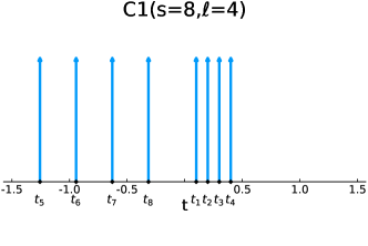
(a) $s=8,\ell=4$, 1 cluster (configuration C1).

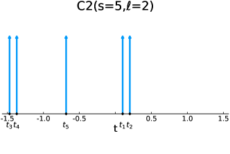
(b) $s=5,\ell=2$, 2 clusters (configuration C2).

Figure 5.1: Examples for the configurations C1 and C2.

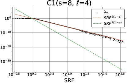
(a) $s=8,\ell=4$, 1 cluster (configuration C1).

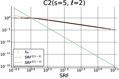
(b) $s=5,\ell=2$, 2 clusters (configuration C2).

Figure 5.2: Decay rate of $\lambda_{\min}$ as a function of $\mathrm{SRF}$. Results of $n=1000$ random experiments with randomly chosen $\Delta,\Omega$ are plotted versus the theoretical bound $\mathrm{SRF}^{2\left(1-\ell\right)}$. The curve $\mathrm{SRF}^{2\left(1-s\right)}$ is shown for comparison. The bound stops to be accurate for $\mathrm{SRF}<O(1)$.

In another experiment (Figure 5.3), we fixed $\Delta,\ell,s$ and changed $\Omega$. As expected, when $\Omega$ became small enough, the left inequality in (3.1) was violated, and indeed we can see that in this case the asymptotic decay was $\approx\mathrm{SRF}^{2\left(1-s\right)}$. See Remark 3.4 for further discussion.

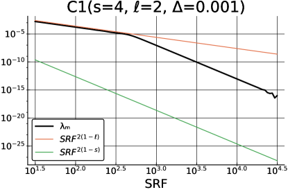
(a) Configuration C1.

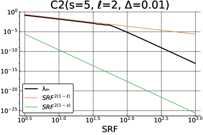
(b) Configuration C2.

Figure 5.3: Breakdown of cluster structure. When $\Omega$ is small enough, the assumptions of Theorem 3.2 are violated for certain $\ell<s$. As a result, the decay rate of $\lambda_{\min}$ corresponds to the entire $\boldsymbol{x}$ being a single cluster of size $\ell=s$. $\Delta$ is kept fixed. See Remark 3.4.

References

- [1] A. Akinshin, D. Batenkov, and Y. Yomdin. Accuracy of spike-train Fourier reconstruction for colliding nodes. In 2015 International Conference on Sampling Theory and Applications (SampTA), pages 617–621, May 2015.
- [2] A. Akinshin, G. Goldman, and Y. Yomdin. Geometry of error amplification in solving Prony system with near-colliding nodes. arXiv preprint arXiv:1701.04058, 2017.
- [3] C. Aubel and H. Bölcskei. Vandermonde matrices with nodes in the unit disk and the large sieve. Applied and Computational Harmonic Analysis, Aug. 2017.
- [4] J. Auton. Investigation of Procedures for Automatic Resonance Extraction from Noisy Transient Electromagnetics Data. Volume III. Translation of Prony’s Original Paper and Bibliography of Prony’s Method. Technical report, Effects Technology Inc., Santa Barbara, CA, 1981.
- [5] D. Batenkov. Complete algebraic reconstruction of piecewise-smooth functions from Fourier data. Mathematics of Computation, 84(295):2329–2350, 2015.
- [6] D. Batenkov. Accurate solution of near-colliding Prony systems via decimation and homotopy continuation. Theoretical Computer Science, 681:27–40, June 2017.
- [7] D. Batenkov. Stability and super-resolution of generalized spike recovery. Applied and Computational Harmonic Analysis, 45(2):299–323, Sept. 2018.
- [8] D. Batenkov, G. Goldman, and Y. Yomdin. Super-resolution of near-colliding point sources. arXiv:1904.09186 [math], Apr. 2019.
- [9] F. Bazán. Conditioning of rectangular Vandermonde matrices with nodes in the unit disk. SIAM Journal on Matrix Analysis and Applications, 21:679, 2000.
- [10] T. Blu, P.-L. Dragotti, M. Vetterli, P. Marziliano, and L. Coulot. Sparse Sampling of Signal Innovations. IEEE Signal Processing Magazine, 25(2):31–40, Mar. 2008.
- [11] E. J. Candès and C. Fernandez-Granda. Super-Resolution from Noisy Data. Journal of Fourier Analysis and Applications, 19(6):1229–1254, Dec. 2013.
- [12] E. J. Candès and C. Fernandez-Granda. Towards a Mathematical Theory of Super-resolution. Communications on Pure and Applied Mathematics, 67(6):906–956, June 2014.
- [13] A. Cuyt, G. Labahn, A. Sidi, and W.-s. Lee. Sparse modelling and multi-exponential analysis (Dagstuhl Seminar 15251). Dagstuhl Reports, 5(6):48–69, 2016.
- [14] Y. de Castro and F. Gamboa. Exact reconstruction using Beurling minimal extrapolation. Journal of Mathematical Analysis and Applications, 395(1):336–354, Nov. 2012.
- [15] L. Demanet and N. Nguyen. The recoverability limit for superresolution via sparsity. 2014.
- [16] D. Donoho. Superresolution via sparsity constraints. SIAM Journal on Mathematical Analysis, 23(5):1309–1331, 1992.
- [17] V. Duval and G. Peyré. Exact Support Recovery for Sparse Spikes Deconvolution. Foundations of Computational Mathematics, 15(5):1315–1355, Oct. 2014.
- [18] A. Fannjiang. Compressive Spectral Estimation with Single-Snapshot ESPRIT: Stability and Resolution. arXiv:1607.01827 [cs, math], July 2016.
- [19] P. Ferreira. Superresolution, the Recovery of Missing Samples, and Vandermonde Matrices on the Unit Circle. 1999.
- [20] S. Fomel. Seismic data decomposition into spectral components using regularized nonstationary autoregression. GEOPHYSICS, 78(6):O69–O76, Oct. 2013.
- [21] W. Gautschi. On inverses of Vandermonde and confluent Vandermonde matrices. Numerische Mathematik, 4(1):117–123, 1962.
- [22] R. A. Horn and C. R. Johnson. Matrix Analysis. Cambridge University Press, Cambridge ; New York, 2nd ed edition, 2012.
- [23] A. E. Ingham. Some trigonometrical inequalities with applications to the theory of series. Mathematische Zeitschrift, 41(1):367–379, Dec. 1936.
- [24] S. Kunis and D. Nagel. On the condition number of Vandermonde matrices with pairs of nearly-colliding nodes. arXiv:1812.08645 [math], Dec. 2018.
- [25] L. Li and T. P. Speed. Parametric deconvolution of positive spike trains. Annals of Statistics, pages 1279–1301, 2000.
- [26] W. Li and W. Liao. Stable super-resolution limit and smallest singular value of restricted Fourier matrices. arXiv:1709.03146 [cs, math], Sept. 2017.
- [27] W. Li, W. Liao, and A. Fannjiang. Super-resolution limit of the ESPRIT algorithm. arXiv:1905.03782 [cs, math], May 2019.
- [28] Y. E. Li and L. Demanet. Phase and amplitude tracking for seismic event separation. Geophysics, 80(6):WD59–WD72, 2015.
- [29] W. Liao and A. Fannjiang. MUSIC for single-snapshot spectral estimation: Stability and super-resolution. Applied and Computational Harmonic Analysis, 40(1):33–67, Jan. 2016.
- [30] A. Moitra. Super-resolution, Extremal Functions and the Condition Number of Vandermonde Matrices. In Proceedings of the Forty-Seventh Annual ACM on Symposium on Theory of Computing, STOC ’15, pages 821–830, New York, NY, USA, 2015. ACM.
- [31] H. L. Montgomery. Ten Lectures on the Interface Between Analytic Number Theory and Harmonic Analysis. American Mathematical Soc., 1994.
- [32] H. L. Montgomery and R. C. Vaughan. Hilbert’s Inequality. Journal of the London Mathematical Society, s2-8(1):73–82, May 1974.
- [33] V. I. Morgenshtern and E. J. Candès. Super-Resolution of Positive Sources: The Discrete Setup. SIAM Journal on Imaging Sciences, 9(1):412–444, Jan. 2016.
- [34] M. Negreanu and E. Zuazua. Discrete Ingham Inequalities and Applications. SIAM Journal on Numerical Analysis, 44(1):412–448, Jan. 2006.
- [35] H. Pan, T. Blu, and M. Vetterli. Towards Generalized FRI Sampling with an Application to Source Resolution in Radioastronomy. IEEE Transactions on Signal Processing, 2016.
- [36] V. Pereyra and G. Scherer. Exponential Data Fitting and Its Applications. Bentham Science Publishers, Jan. 2010.
- [37] T. Peter, D. Potts, and M. Tasche. Nonlinear approximation by sums of exponentials and translates. SIAM Journal on Scientific Computing, 33(4):1920, 2011.
- [38] D. Potts and M. Tasche. Error Estimates for the ESPRIT Algorithm. In D. A. Bini, T. Ehrhardt, A. Y. Karlovich, and I. Spitkovsky, editors, Large Truncated Toeplitz Matrices, Toeplitz Operators, and Related Topics, volume 259, pages 621–648. Springer International Publishing, Cham, 2017.
- [39] M. Reynolds, G. Beylkin, and L. Monzón. On generalized Gaussian quadratures for bandlimited exponentials. Applied and Computational Harmonic Analysis, 34(3):352–365, May 2013.
- [40] D. Slepian. Prolate spheroidal wave functions, Fourier analysis, and uncertainty – V: The discrete case. Bell System Technical Journal, The, 57(5):1371–1430, May 1978.
- [41] D. Slepian. Some Comments on Fourier Analysis, Uncertainty and Modeling. SIAM Review, 25(3):379–393, 1983.
- [42] P. Stoica and R. Moses. Spectral Analysis of Signals. Pearson/Prentice Hall, 2005.
- [43] J. Varah. The prolate matrix. Linear Algebra and its Applications, 187:269–278, July 1993.