Compiled (100.6640) Superresolution; (110.3055) Information theoretical analysis; (120.3940) Metrology.

Tempering Rayleigh’s curse with PSF shaping

Abstract

It has been argued that, for a spatially invariant imaging system, the information one can gain about the separation of two incoherent point sources decays quadratically to zero with decreasing separation, an effect termed Rayleigh’s curse. Contrary to this belief, we identify a class of point spread functions with a linear information decrease. Moreover, we show that any well-behaved symmetric point spread function can be converted into such a form with a simple nonabsorbing signum filter. We experimentally demonstrate significant superresolution capabilities based on this idea.

Rayleigh’s criterion, which stipulates a minimum separation for two equally bright incoherent point light sources to be distinguishable by an imaging system, is based on heuristic notions. A more accurate approach to optical resolution can be formulated in terms of the Fisher information and the associated Cramér-Rao lower bound (CRLB), which sets a limit on the precision with which the separation can be estimated [1]. Using statistical methods, it has been found that the resolution predicted by Rayleigh’s criterion has been routinely improved [2, 3].

A recent reexamination of the problem by Tsang and coworkers [4, 5, 6, 7] showed that, for direct imaging, the Fisher information drops quadratically with the object separation. In consequence, the variance of any estimator based in these intensity-based measurements diverges, giving rise to the so-called Rayleigh’s curse [4]. Surprisingly, when one calculates the quantum Fisher information [8] (i.e., optimized over all the possible measurements), the associated quantum CRLB maintains a constant value. This shows that, in principle, the separation can be estimated with precision unaffected by Rayleigh’s curse. The key ingredient for this purpose is to utilize phase-sensitive measurements [9, 10]. This has been demonstrated by holographic mode projection [11], heterodyne detection [12, 13], and parity-sensitive interferometers [14].

These experiments dispel Rayleigh’s curse, but require sophisticated equipment. In this Letter, we revisit the scenario of direct detection, for it is the cut-and-dried method used in the laboratory. We show that by using a simple phase mask—a signum filter—direct detection makes the Fisher information drop linearly. This scaling law opens new avenues for boosting resolution, as we demonstrate here with a proof-of-principle experiment. Moreover, this means that the advantage of the aforementioned quantum schemes, with a separation-independent Fisher information, over classical techniques is smaller than previously thought.

We work with a spatially invariant imaging system and two equally bright incoherent point sources separated by a distance $\mathfrak{s}$. We assume quasimonochromatic paraxial waves with one specified polarization and one spatial dimension, with $x$ denoting the image-plane coordinate in direction of the separation. This simplified 1D geometry is sufficient to make clear our procedure and it works for some applications, such as, e.g., spectroscopy. The more realistic 2D case can be worked along the same lines, although at the price of dealing with a two-parameter estimation.

If $I(x)$ is the spatial distribution of the intensity in the image from a point source, commonly called the point-spread function (PSF) [15], the direct image can be written as

$$p(x|\mathfrak{s})=\frac{1}{2}[I(x-\mathfrak{s}/2)+I(x+\mathfrak{s}/2)]\,,$$ (1)

where $p(x|\mathfrak{s})$ is the probability density for detecting light at $x$ conditional on the value of $\mathfrak{s}$. We model light emission (detection) as a random process (shot noise) [16]. The precision in estimating $\mathfrak{s}$ is governed by the Fisher information

$$F(\mathfrak{s})=N\int\frac{[\partial_{\mathfrak{s}}p(x|\mathfrak{s})]^{2}}{p(x|\mathfrak{s})}\,dx,$$ (2)

where $\partial_{\mathfrak{s}}$ is the partial derivative with respect to $\mathfrak{s}$. In this stochastic scenario, $N$ is the number of detections, which can be approximately taken as Poissonian with a mean $Np(x|\mathfrak{s})dx$. Without loss of generality, we set $N=1$ and evaluate the Fisher information per single detection. Reintroducing $N$ into the final results is always straightforward. The CRLB ensures that the variance of any unbiased estimator $\hat{\mathfrak{s}}$ of the quantity $\mathfrak{s}$ is bounded by the reciprocal of the Fisher information; viz, $(\Delta\hat{\mathfrak{s}})^{2}\geq 1/F(\mathfrak{s})$.

Since we are chiefly interested in the case of small separations, we expand $p(x|\mathfrak{s})$ in $\mathfrak{s}$, getting $p(x|\mathfrak{s})=I(x)+I^{\prime\prime}(x)/8\,\mathfrak{s}^{2}+O(\mathfrak{s}^{4})$, where a prime denotes derivative respect to the variable. Observe that the odd powers of $\mathfrak{s}$ make no contribution, because the contributions from the two PSF components cancel each other. The associated Fisher information becomes

$$F(\mathfrak{s})=\frac{\mathfrak{s}^{2}}{16}\int\left\{\frac{[I^{\prime\prime}(x)]^{2}}{I(x)}+O(\mathfrak{s}^{2})\right\}\,dx\,.$$ (3)

Commuting the order of integration and summation immediately yields a quadratic behavior for all PSFs: $F(\mathfrak{s})\propto\mathfrak{s}^{2}+O(\mathfrak{s}^{4})$. However, such an operation is not always admissible [17], which leaves room for tempering Rayleigh’s curse with PSF shaping techniques.

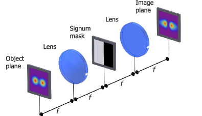
Figure 1: Scheme of an optical coherent $4f$ processor, with a signum mask in the Fourier plane.

To illustrate this point, let us assume, for the time being, that our PSF is well approximated by a parabolic profile near the origin; i.e., $I(x)\simeq\alpha x^{2}$, which implies

$$p(x|\mathrm{s})\simeq\alpha(x^{2}+\mathfrak{s}^{2}/4)\,,\qquad x,\mathfrak{s}\ll 1\,.$$ (4)

When this holds true, the integrand in (2) reduces to a Lorentzian function

$$F(\mathfrak{s})\simeq\int\frac{\alpha^{2}\mathfrak{s}^{2}}{4x^{2}+\mathfrak{s}^{2}}\,dx\,.$$ (5)

Because of the strong peak at $x=0$, when $\mathfrak{s}\ll 1$ the tails of the Lorentzian do not contribute appreciably and can be ignored. As a result, we get

$$F(\mathfrak{s})\simeq\lambda\,\mathfrak{s}\,,$$ (6)

with $\lambda=\pi\alpha/2$, and the information is indeed linear rather than quadratic at small separations. Note that the proper normalization of $p(x|\mathfrak{s})$ is guaranteed by higher-order terms in the expansion (4), but they do not affect the scaling in (6).

Next, we show that any PSF can be converted to the form (5) by applying a simple nonabsorbing spatial filter at the output of the system. In what follows, $\Psi(x)$ indicates the amplitude PSF, so that $I(x)=|\Psi(x)|^{2}$, and $\Psi(f)$ its Fourier transform. We process the image by a coherent processor, such as, e.g., a standard $4f$ system [15] schematized in Fig. 1. In the Fourier plane, each point source gives rise to $\Psi(x\pm\mathfrak{s}/2)\mapsto\Psi(f)e^{\pm i\pi fs}$. In that plane, we apply a signum mask: $\mathrm{sgn}(f)\Psi(f)e^{\pm i\pi fs}$, where for a real number $\operatorname{sgn}(t)=|t|/t$ for $t\neq 0$ and $\operatorname{sgn}(0)=0$. As the signum is a pure phase filter, no photons are absorbed. The signal components are then convolved with the inverse Fourier transform of the signum function, which is $\mathcal{F}^{-1}\{\mathrm{sgn}(f)\}=-i/(\pi x)$. In this way, the processor performs

$$\Psi^{\mathrm{sgn}}_{\pm}(x,\mathfrak{s})=-\frac{i}{\pi}\int\frac{\Psi(x^{\prime}\pm\mathfrak{s}/2)}{x-x^{\prime}}\,dx^{\prime}\,.$$ (7)

which is the Hilbert transform of the signal. The optical implementation of this transform has a long history [18, 19, 20]. It has been used in several fields, but most prominently in image processing for edge enhancement, because it emphasizes the derivatives of the image.

Applying the change of variable $\xi=x^{\prime}-x$, expanding $\Psi$ to the second order in the small quantity $x\pm\mathfrak{s}/2$, and using the spatial symmetry of $\Psi$, we approximate the output amplitudes after the signum mask by

$$\Psi^{\mathrm{sgn}}_{\pm}(x,\mathfrak{s})\simeq\frac{i}{\pi}(x\pm\mathfrak{s}/2)\int\frac{\Psi^{\prime}(\xi)}{\xi}\,d\xi\,,\qquad x,\mathfrak{s}\ll 1.$$ (8)

The detection probability density near the origin now takes the parabolic shape, as discussed before, viz,

$$p^{\mathrm{sgn}}(x|\mathfrak{s})=\frac{1}{2}\left[|\Psi^{\mathrm{sgn}}_{-}(x,\mathfrak{s})|^{2}+|\Psi^{\mathrm{sgn}}_{+}(x,\mathfrak{s})|^{2}\right]\simeq\alpha(x^{2}+\mathfrak{s}^{2}/4),$$ (9)

with $\alpha=[\int\Psi^{\prime}(\xi)/\xi\,d\xi]^{2}/\pi^{2}$. Note carefully that the parabolic behavior (9) is general, but the value of the coefficient $\alpha$ depends on the explicit form of the PSF $\Psi(x)$. We thus have a linear Fisher information as in (6). In physical terms, this happens because the Fourier-space processing incorporates phase information. In addition, the combined system consisting of the imaging and PSF reshaping step remains spatially invariant and so the information about the separation is not degraded by misaligning the signal and detection devices, as it happens, for example, when the centroid of the two-component signal is not perfectly controlled.

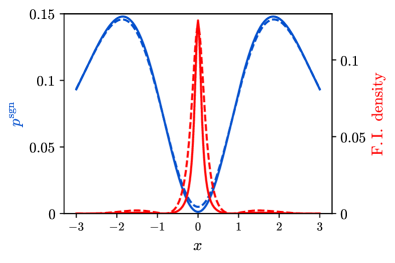
Figure 2: Detection probabilities (blue) and Fisher information density [i.e., the integrand in the definition (2)] (red) corresponding to a Gaussian PSF modified by the signum filter for separations $0.2\sigma$ (solid lines) and $0.4\sigma$ (broken lines). Here, and in all the figures, length is in units of $\sigma$.

We recall that the Hilbert transform is the essential tool for getting the dispersion relations [21], which relate the real and imaginary parts of the response function (i.e., susceptibility) of a linear causal system. If we think of $\Psi(x)$ as an absorption profile near resonance , we realize that the real part of susceptibility shows anomalous dispersion—linear slope—near the resonance: after squaring we then get a parabolic $p(x,\mathfrak{s})$ near the origin.

Let us ellaborate our proposal with the relevant example of a system characterized by a Gaussian PSF: $\Psi(x)=(2\pi\sigma^{2})^{-1/4}\exp(-\tfrac{1}{4}x^{2}/\sigma^{2})$, where $\sigma$ is an effective width that depends on the wavelength. Henceforth, we take $\sigma$ as our basic unit length, so the corresponding magnitudes (such as separation, variance, etc) appear as dimensionless. Apart from its computational efficiency, the Gaussian PSF approximates fairly well the Airy distribution when the illumination is done by a Gaussian distribution that apodises the circular aperture.

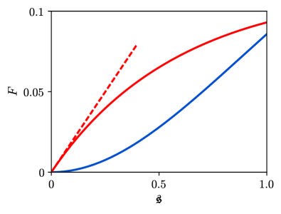
Figure 3: Fisher information about separation for imaging with a Gaussian PSF with (red concave line) and without (blue convex line) the signum filter. The asymptotic behavior of the superresolution given by the right hand side of (12) is also shown (broken red line).

The Fisher information associated with the direct imaging is obtained from (2); the result reads

$$F_{\mathrm{direct}}(\mathfrak{s})\simeq\frac{(\mathfrak{s}/\sigma)^{2}}{8\sigma^{2}}\,,$$ (10)

confirming once again the quadratic scaling of Rayleigh’s curse. This is to be compared with the information accessible by signum-filter enhanced detection. We first perform the Hilbert transform of the Gaussian PSF;

$$|\Psi^{\mathrm{sgn}}_{\pm}(x,\mathfrak{s})|^{2}=\frac{2\sqrt{2}\;D\left(\frac{x\pm\mathfrak{s}/2}{2\sigma}\right)^{2}}{\pi^{3/2}\sigma}\,,$$ (11)

where $D(z)$ denotes Dawson’s integral [22]. Similar results have been reported for the dispersion relations of a Gaussian profile [23]. In particular, $D(-z)=-D(z)$ and $D(z)\simeq z(1-\tfrac{2}{3}z^{2})$ for $z\rightarrow 0$, so the dominant behavior is indeed linear. Therefore, the expansion in (9) holds with $\alpha=(2\pi^{3})^{-1/2}\sigma^{-3}$ and, in consequence,

$$F^{\mathrm{sgn}}(\mathfrak{s})\simeq\frac{(\mathfrak{s}/\sigma)}{2\sqrt{2\pi}\sigma^{2}}\,.$$ (12)

The detection probabilities and Fisher information densities typical for a signum-enhanced detection with a Gaussian PSF are shown in Fig. 2 for two different values of $\sigma$. Notice that nonzero separation is evidenced by nonzero readings at the center of the image. Interestingly, most of the information on the separation comes from detections near the origin and this region shrinks with decreasing $\mathfrak{s}$.

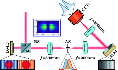
Figure 4: Experimental setup. The notations used are as follows: DMD: digital micromirror chip, BS: beam-splitter, AS: aperture stop at the Fourier plane of the lens, and SLM: spatial light modulator. In the inset, we show a typical intensity scan recorded with zero separation setting and a total detection count of $434,000$. The separation is estimated from the total number of detections registered in the central pixel column.

The superresolution potential of our technique is illustrated in Fig. 3. The linear scaling can provide big advantages in terms of the resources required to measure very small separations. For example, to measure a $10\times$ smaller separation to a given precision requires $100\times$ more detection events with the conventional setup, while just $10\times$ would do with the new technique. For a fixed photon flux this translates into shorter detection times. At the same time, the new technique is simple to implement in existing imaging devices, such as telescopes, microscopes or spectrometers.

We have implemented the method with the setup sketched in Fig. 4. Two mutually incoherent equally bright point sources were generated with a controlled separation. After preparation, this signal was detected using a signum spatial-frequency filter, by which the original Gauss PSF is reshaped into the Dawson form as in (11).

A spatially coherent, intensity-stabilised Gaussian beam was used to illuminate a digital micro-mirror chip (DMD, Texas Instruments) with a mirror pitch of $10\leavevmode\nobreak\ \mu$m. Two sinusoidal grating patterns with very close spatial frequencies were created by the DMD, which allows for a very precise control of the angular separation in a chosen diffraction order. Angular separations as small as $4.6\leavevmode\nobreak\ \mu$rad were realized; these correspond to a linear separation of 0.042$\sigma$. To ensure incoherence, one pattern was ON at a time, while keeping the switching time well below the detector time resolution. Imaging with an objective of focal length $f=300$ mm gave rise to two spatially separated Gaussian spots of $\sigma=33.2\leavevmode\nobreak\ \mu$m. An aperture stop was used to cut-off unwanted diffraction orders. This completes the direct imaging stage.

In the signum-enhanced imaging part, a phase spatial light modulator (SLM) (Hammamatsu) with square pixels of $20\times 20\leavevmode\nobreak\ \mu$m was operated in the Fourier plane of a standard $4f$ optical system. The SLM implemented the signum mask hologram calculated as an interference pattern between a phase unit-step and a blaze grating, allowing for over $0.9$ transfer efficiency. Finally, the output signal was measured by a CCD camera (Basler) with $7.4\times 7.4\leavevmode\nobreak\ \mu$m pixels positioned at the output of the $4f$ processor. Vertical $4$-pixel binning was activated to reduce the readout noise, so the effective pixel size is $7.4\times 29.6\leavevmode\nobreak\ \mu$m. The corresponding signals used in the reconstruction process, resulting from summing three pixels, were in the range of 120–253 photoelectrons, in comparison to a sum of $3\times 7$ photoelectron readout noise. The camera exposure time was set to $100$ ms to keep the dark noise contribution negligible.

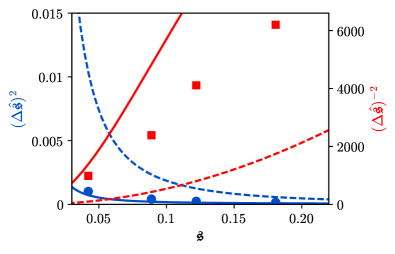
Figure 5: Experimental variances of the separation estimator (blue dots) compared with the direct detection (blue broken line) and the signum-enhanced limit (solid blue line). The latter is corrected for the finite pixel size of $7.6\leavevmode\nobreak\ \mu$m. For completeness, the reciprocal of the variances, called the precisions, are shown in red.

Several separations, ranging from about $0.042\sigma$ ($1.4\leavevmode\nobreak\ \mu$m) to $0.18\sigma$ ($6\leavevmode\nobreak\ \mu$m), were measured. Two hundred intensity scans were recorded for each separation setting. One typical 2D scan is shown in the inset of Fig. 4. Since the two incoherent points are separated horizontally, no information about separation is lost by collecting pixel counts column-wise. The resulting 1D projections are samples from the theoretical intensity distribution $p^{\mathrm{sgn}}(x,\mathfrak{s})$, see Fig. 2. Notice that for small separations only the central parts of the projections contribute significant information. In particular all pixel columns, except the central one, can be ignored in the raw data in the inset of Fig. 4. Therefore, each 2D intensity scan is reduced to a single datum—the total number of detections in the central pixel column.

We express the response of the real measurement by a second-order polynomial on the separation $p^{\mathrm{}}(\mathfrak{s})=a+b\mathfrak{s}^{2}$ and estimate the coefficients from a best fit of the mean experimental detections. For each separation, we calculate the estimator mean $\langle\widehat{\mathfrak{s}}\rangle$ and variance$(\Delta\widehat{\mathfrak{s}})^{2}$.

Experimental results are summarized in Figs. 5 and 6. Figure 5 compares the experimentally determined variances with the theoretical limits of the direct and signum-enhanced imaging for a Gaussian PSF and $434,000$ detections per measurement. Reciprocal quantities (precisions) are also shown. Signum-enhanced imaging clearly breaks the quadratic Rayleigh’s curse in the whole range of measured separations, with an variance improvements up to $10\times$ compared with the direct imaging. Notice also the apparent linear behavior of experimental precisions (red symbols) as compared to the quadratic lower bound predicted for the direct imaging (red broken line).

More estimator statistics is shown in Fig. 6. Experimental estimates are nearly unbiased and not much worse than the theoretical limit calculated for the finite pixel size used in the experiment. Engineering the PSF brings about reliable separation estimates in the region where direct imaging fails, as for example for separations $\mathfrak{s}\lessapprox 0.07\sigma$ in Fig. 6.

In summary, we have demonstrated a robust experimental violation of Rayleigh’s curse. Experimental imperfections prevent one from achieving the ultimate limit shown in Fig. 3. For larger separations, systematic errors and setup instability make important contributions to the total (small) error. For very small separations, the measured signal is very weak and background noise becomes the limiting factor. Further improvements are possible by optimizing the noise statistics and resolution of the camera.

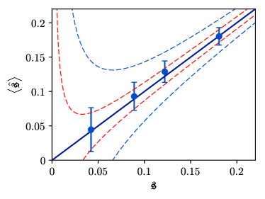
Figure 6: Estimation of the separation from signum-enhanced imaging. Estimator means (dots) and standard deviations (error bars) are shown. Same statistics is provided for the best unbiased estimators from direct (blue lines) and signum-enhanced (red lines) imaging as given by the CRLB. The latter takes in account the finite pixel size used in the experiment.

Finally, one could wonder whether a different filter could yield a better scaling of the Fisher information using direct imaging. The dispersion relations suggest that this behavior is largely determined by the zeros of the PSF. Additional work is needed to explore all these issues, but the simplicity of the signum mask makes it very attractive for superresolution applications.

We acknowledge financial support from the Grant Agency of the Czech Republic (Grant No. 18-04291S), the Palacký University (Grant No. IGA_PrF_2018_003), the European Space Agency’s ARIADNA scheme, and the Spanish MINECO (Grant FIS2015-67963-P).

References

- [1] S. M. Kay, Fundamentals of Statistical Signal Processing, vol. 1 (Prentice Hall, 1993).
- [2] A. J. den Dekker and A. van den Bos, J. Opt. Soc. Am. A 14, 547 (1997).
- [3] P. R. Hemmer and T. Zapata, J. Opt. 14, 083002 (2012).
- [4] M. Tsang, R. Nair, and X.-M. Lu, Phys. Rev. X 6, 031033 (2016).
- [5] R. Nair and M. Tsang, Phys. Rev. Lett. 117, 190801 (2016).
- [6] R. Nair and M. Tsang, Opt. Express 24, 3684 (2016).
- [7] M. Tsang, New J. Phys. 19, 023054 (2017).
- [8] D. Petz and C. Ghinea, Introduction to Quantum Fisher Information (World Scientific, 2011), pp. 261–281.
- [9] C. Lupo and S. Pirandola, Phys. Rev. Lett. 117, 190802 (2016).
- [10] J. Rehacek, M. Paúr, B. Stoklasa, Z. Hradil, and L. L. Sánchez-Soto, Opt. Lett. 42, 231 (2017).
- [11] M. Paur, B. Stoklasa, Z. Hradil, L. L. Sanchez-Soto, and J. Rehacek, Optica 3, 1144 (2016).
- [12] F. Yang, A. Taschilina, E. S. Moiseev, C. Simon, and A. I. Lvovsky, Optica 3, 1148 (2016).
- [13] F. Yang, R. Nair, M. Tsang, C. Simon, and A. I. Lvovsky, Phys. Rev. A 96, 063829 (2017).
- [14] W. K. Tham, H. Ferretti, and A. M. Steinberg, Phys. Rev. Lett. 118, 070801 (2016).
- [15] J. W. Goodman, Introduction to Fourier Optics (Roberts and Company, 2004).
- [16] S. Ram, E. Sally Ward, and R. J. Ober, PNAS 103, 4457 (2006).
- [17] H. L. Royden, Real Analysis (Prentice Hall, 1988).
- [18] A. Kastler, Rev. Opt. 29, 308 (1950).
- [19] H. Wolter, Ann. Phys. 7, 341 (1950).
- [20] A. W. Lohmann, D. Mendlovic, and Z. Zalevsky, Opt. Lett. 21, 281 (1996).
- [21] F. W. King, Hilbert transforms (Cambridge University Press, 2009).
- [22] N. M. Temme, NIST Handbook of Mathematical Functions (Cambridge University Press, 2010), chap. Error Functions, Dawson’s and Fresnel Integrals.
- [23] R. J. Wells, J. Quant. Spect. Rad. Transfer 62, 29 (1999).