On the relationship between metallicity distributions of globular clusters and of circumgalactic gas

Abstract

The abundance of alpha elements and iron in stars of globular clusters (GCs) shows the composition of the gaseous medium, in which they have been formed. In the present paper, we discuss a possibility to consider dense clouds of circumgalactic gas (partial Lyman limit systems and Lyman limit systems) observed in the 100 – 130 kpc neighbourhood of galaxies at redshifts of $\rm 0.1<z<1.1$ as being the residual parts of clouds, in which globular clusters have been formed. Conclusions have been drawn based on statistical analysis of the abundance of magnesium and iron in GCs and in circumgalactic clouds and on the spatial location of objects of both types.

1 Introduction

Interpretation of conditions in which globular clusters (GCs) of ours and other galaxies were formed is a field of intense studies by present-day astrophysics, in which there are still many unsolved issues. Over the past decade, significant progress has been made in understanding the properties of GCs and the conditions in which they were formed (see the review by Kruijssen (2014)).

It has long been established in the number of studies that GCs of the Galaxy are divided into two distinct subsystems: metal-rich and metal-poor in terms of iron (Harris, 1996; Dias et al., 2016; Carretta et al., 2010) and magnesium abundances (Dias et al., 2016; Carretta et al., 2010; Pritzl et al., 2005). This result confirms the earlier result obtained on the basis of the study of metallicity (Marsakov & Suchkov, 1977; Zinn, 1985). The data, suitable for statistical analysis of the abundance of iron and magnesium in GCs, allow us to make significant progress in the study of early stages of evolution of galaxies. It was argued that these elements are produced by two different types of supernovae mainly (Woosley & Weaver, 1995; Tsujimoto et al., 1995; Limongi & Chieffi, 2003; Hirschi et al., 2005): magnesium is formed as a result of explosions of core-collapse supernovae (SNe CC), iron is formed by type I a supernovae (SNe Ia).

The average ages of GCs in the metal-rich and the metal-poor groups are similar (Marin-Franch et al., 2009; VandenBerg et al., 2013; Carretta et al., 2010; Chattopadhyay et al., 2012) within measurement errors which can reach 25%. According to Chattopadhyay et al. (2012), the mean age of the metal-rich Galactic and M31 GCs is $10.6\pm 0.5$ Gyr, and the mean age of the metal-poor Galactic and M31 GCs is $10.2\pm 0.2$ Gyr. It follows therefrom that the enrichment of gas with magnesium and iron occurred quickly. There is nothing surprising in this rapid enrichment by magnesium: the lifetime of SNe CC progenitors from birth to explosion is only a few million years. Rapid iron enrichment was difficult to explain up to and including 2005, because it is thought that the time interval from the moment of formation and up to the explosion in SNe Ia progenitors is about 1.5 billion years, and they massively have exploded in 3 billion years (Dahlen et al., 2004; Strolger et al., 2005). It has been established in recent years that the age of SNe Ia progenitors is $T<500$ Myr and the frequency of SNe Ia explosions in star-forming regions is 3-5 times higher than the corresponding frequency in the representatives of old stellar populations (Mannucci et al., 2006; Brandt et al., 2010; Li et al., 2011; Maoz et al., 2014; Rodney et al., 2014; Andersen & Hjorth, 2018).

The present study discusses a possibility to consider circumgalactic clouds (partial Lyman limit systems, pLLSs, with neutral hydrogen column densities in the range $16.1<logN_{HI}<17.2$ and Lyman limit systems, LLSs, $17.2<logN_{HI}<17.7$) observed in the 100–130 kpc vicinity from galaxies at redshifts of $\rm 0.1<z<1.1$ as the relic of the gaseous medium, from which GCs were formed. LLSs and pLLSs are highly ionised gaseous structures in distinction to more dense Damped Ly$\alpha$ systems (DLAs; $logN_{HI}>20.3$) which are partly neutral. LLSs and pLLSs are expected to probe cool, dense streams through the circumgalactic medium of galaxies ((Wotta et al., 2016) and references therein). In 2013, the results of the first large-scale studies of the chemical element abundance in clouds that appeared in the line of sight of quasars were obtained (Lehner et al., 2013). These studies were continued in a series of papers (Wotta et al., 2016; Lehner et al., 2016). It has been found that the magnesium abundance distribution estimated from 55 clouds is bimodal, i.e., the distribution function has two distinct peaks with the deep minimum at $\rm\mbox{[Mg/H]}\sim-0.9$. The statistics of these studies allows us to draw important conclusions which will be discussed in the paper.

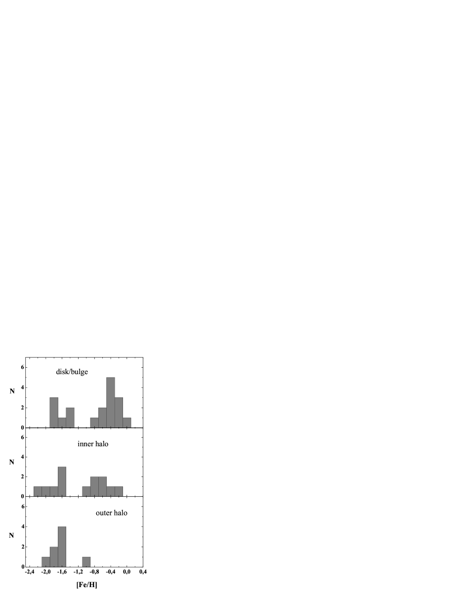
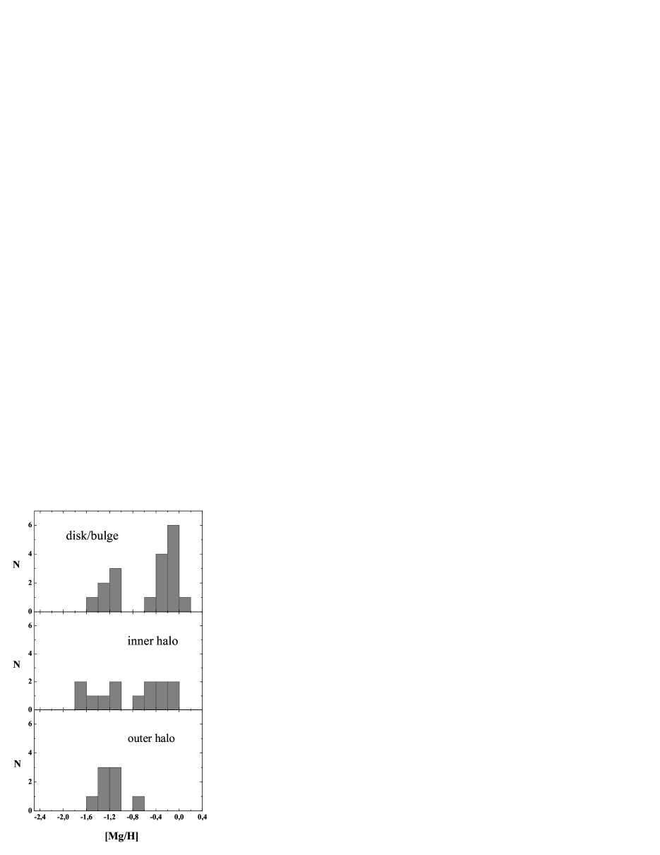
Figure 1: Histograms of iron (left-hand) and magnesium (right-hand)abundances in GCs built using the data from Dias et al. (2016) for objects of three subsystems of the Galaxy: disk/bulge objects, of the inner and outer halos.

2 Statistical analysis of iron and magnesium abundances in globular clusters

Our conclusions about the abundance of chemical elements in GCs are based on analysing the results of the studies presented in three papers: Dias et al. (2016); Carretta et al. (2010); Pritzl et al. (2005). The paper by Dias et al. (2016) presents a sample of fifty one Galactic GCs with parameters determined using one method. The abundances of two chemical elements of interest, [Fe/H] and [Mg/H], were determined using the MILES library. The authors divided clusters into three groups according to the criteria proposed in Carretta et al. (2010): objects of the disc/bulge and of the inner and outer halos. As can be seen from the analysis of histograms built separately for disc/bulge and inner halo objects (see Fig. 1), the distributions are bimodal with a deep minimum at $\mbox{[Fe/H]}\sim-1.2$ ($\mbox{[Mg/H]}\sim-0.9$). Tables 1 and 2 give average values of the iron and magnesium abundance, root-mean-square deviations, and the number of GCs in each group. Let us note that iron-poor clusters coincide with those being magnesium-poor.

Let us proceed to the study carried out by Carretta et al. (2010). In that paper, 139 GCs from the Harris catalogue (Harris, 1996) were divided into three groups on the basis of the cluster velocity and their position in the Galaxy. To the outer halo, twenty eight GCs were assigned, to the inner halo – thirty five GCs, to the disc with a bulge – seventy six GCs. The histograms of the iron abundance in the GCs of three groups are shown in Fig. 2. It can be noticed that two sub-populations are clearly seen only in the disc/bulge group: metal-poor consisting of thirty nine GCs with the average value $\rm\langle\mbox{[Fe/H]}\rangle=-1.50$ and metal-rich consisting of thirty seven GCs with the average value $\rm\langle\mbox{[Fe/H]}\rangle=-0.44$. Between two cluster groups, there is a deep minimum in the vicinity of $\rm\mbox{[Fe/H]}\sim-1.2$. Objects of the outer and inner halos have a number of measurements sufficient for statistical analysis in the metal-poor region only. Mean values of the iron abundance, the root-mean-square deviations, and the number of GCs in each group are given in Tables 1 and 2.

In the paper by Carretta et al. (2010), [Mg/H] were additionally determined for nineteen GCs. Fifteen of them are metal-poor with $\rm\mbox{[Fe/H]}<-0.9$. This group of clusters includes objects of both the halo and disc subsystems. Taking into consideration a small number of GCs, we did not divide them into subgroups and built histograms for the entire sample (Fig. 3). The average values and standard deviations in the metal-poor and metal-rich regions are given in Tables 1 and 2.

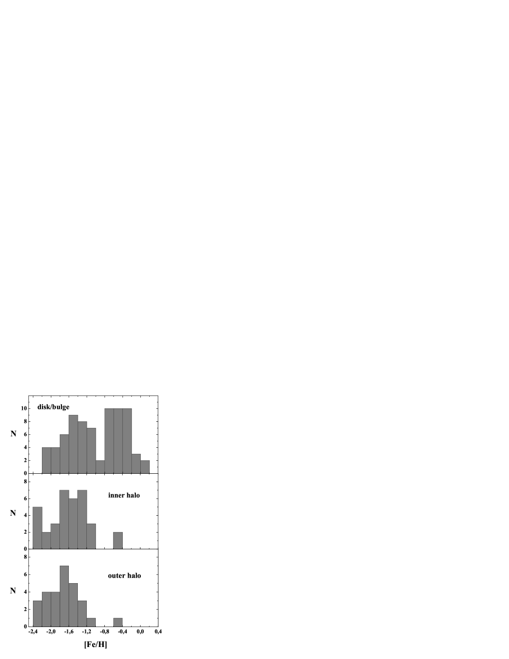
Figure 2: Distribution of the iron abundance in GCs built from the Carretta et al. (2010) data for the objects of three subgroups of GCs in our Galaxy: objects of the disc/bulge and of the inner and outer halos.

Table 1: Iron abundance in globular clusters.

subsystem	metal-poor group			metal-rich group
in the Galaxy
	$<\mbox{[Fe/H]}>$	$\sigma(\mbox{[Fe/H]})$	number of GCs	$<\mbox{[Fe/H]}>$	$\sigma(\mbox{[Fe/H]})$	number of GCs
Carretta et al. 2010
19 GCs with	-1.69	0.41	14	-0.62	0.17	5
measured [Mg/H]
inner halo	-1.67	0.37	33	–	–	2
outer halo	-1.74	0.32	27	–	–	1
disc/bulge	-1.50	0.33	39	-0.44	0.26	37
Dias et al. 2016
inner halo	-1.78	0.24	6	-0.64	0.24	7
outer halo	-1.70	0.13	7	–	–	1
disc/bulge	-1.65	0.14	6	-0.38	0.21	12
Pritzl et al. 2005
halo	-1.73	0.37	32	-0.54	0.20	3
disc/bulge	-	-	-	-0.55	0.29	6

Table 2: Magnesium abundance in globular clusters and circumgalactic clouds.

subsystem	metal-poor group			metal-rich group
in the Galaxy
	$<\mbox{[Mg/H]}>$	$\sigma(\mbox{[Mg/H]})$	number of GCs	$<\mbox{[Mg/H]}>$	$\sigma(\mbox{[Mg/H]})$	number of GCs
Carretta et al. 2010
19 GCs with	-1.19	0.35	15	-0.17	0.15	4
measured [Mg/H]
Dias et al. 2016
inner halo	-1.37	0.25	6	-0.37	0.17	7
outer halo	-1.27	0.13	7	–	–	1
disc/bulge	-1.21	0.15	6	-0.19	0.14	12
Pritzl et al. 2005
halo	-1.38	0.42	33	–	–	2
disc/bulge	–	–	–	-0.24	0.23	6
Wotta et al. 2016
pLLSs	-1.58	0.23	24	-0.34	0.28	20
pLLSs$+$	-1.49	0.28	32	-0.38	0.30	22
LLSs

Let us turn to another study performed in Pritzl et al. (2005). It shows determinations of the abundances of chemical elements in forty five GCs obtained by several groups of authors based on high-resolution spectroscopy of red giants (see Tables 1 and 2 in their paper). For most GCs, the abundance of a chemical element in question was performed by different authors. We used the average values in their Table 2. For our purpose, we need GCs with the iron and magnesium abundances measured. Such data are available for forty one GCs. The clusters belong to different galactic subsystems. According to the criteria proposed in the paper by Mackey & Gilmore (2004), nineteen GCs are classified as belonging to the disc/bulge subsystem including the thick disc, the rest – to the halo subsystem. In compliance with the studies of the cluster-velocity components (Pritzl et al., 2005), six GCs are referred to the disc/bulge subsystem, the rest of objects were divided into the young and old halo subsystems, including 3 objects of the Sagittarius dSph galaxy (M54, Ter7, Pal12). Comparing both classifications, one can notice that according to Pritzl et al. (2005) the halo objects are referred to thick-disc objects, while according to Mackey & Gilmore (2004) all them belong to the metal-poor subgroup with the exception of three GC: Ter7, Pal 12, and NGC6553. For our purpose, it is necessary to determine the average abundance of iron and magnesium for the metal-poor and metal-rich components of a GC, thus, we confine ourselves to analysing the properties of GCs divided into groups in compliance with the classification presented in Pritzl et al. (2005). Tables 1 and 2 show the average abundance, root-mean-square deviations, and the number of clusters in the metal-poor and metal-rich subgroups.

The bimodal metallicity distribution of GCs is also observed in other massive galaxies. It is known, for example, that in the Virgo Cluster galaxies the metallicity distribution of GCs is also bimodal with the average metallicity slightly depending on the parent galaxy mass and close to the GC metallicity distribution in our Galaxy (Kruijssen, 2014). The metallicity distribution of GCs in M31 and of ultracompact dwarf galaxies also complies with this conclusion (Chattopadhyay et al. (2012) and references therein).

The average iron and magnesium abundances of metal-poor GCs determined by the results of all the authors, weighted according to the number of objects, are $\rm\langle\mbox{[Fe/H]}\rangle=-1.66\pm 0.34$, $\rm\langle\mbox{[Mg/H]}\rangle=-1.31\pm 0.35$. The same for metal-rich GCs: $\rm\langle\mbox{[Fe/H]}\rangle=-0.47\pm 0.25$, $\rm\langle\mbox{[Mg/H]}\rangle=-0.24\pm 0.18$.

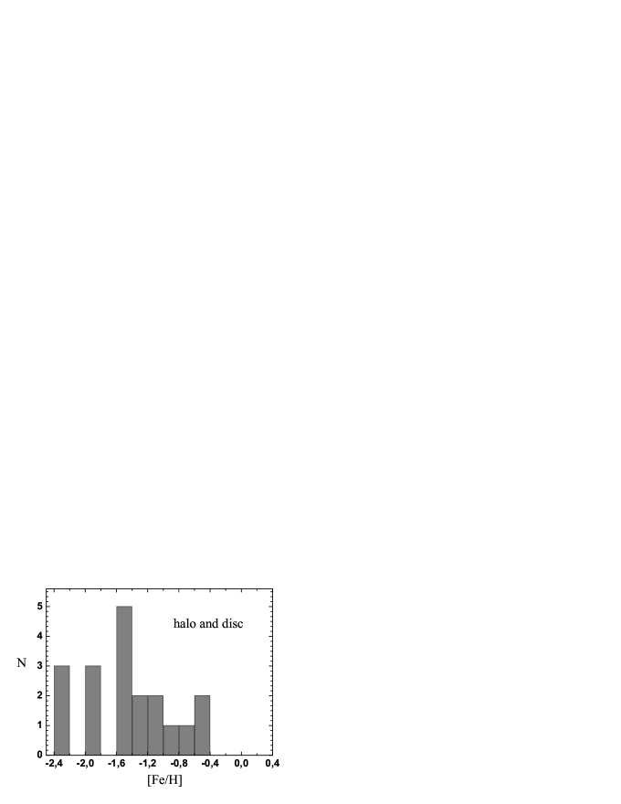
Figure 3: Distributions of iron (left-hand) and magnesium (right-hand) abundances for nineteen GCs of both the halo and disk subsystems from Carretta et al. (2010), for which magnesium abundances are measured.

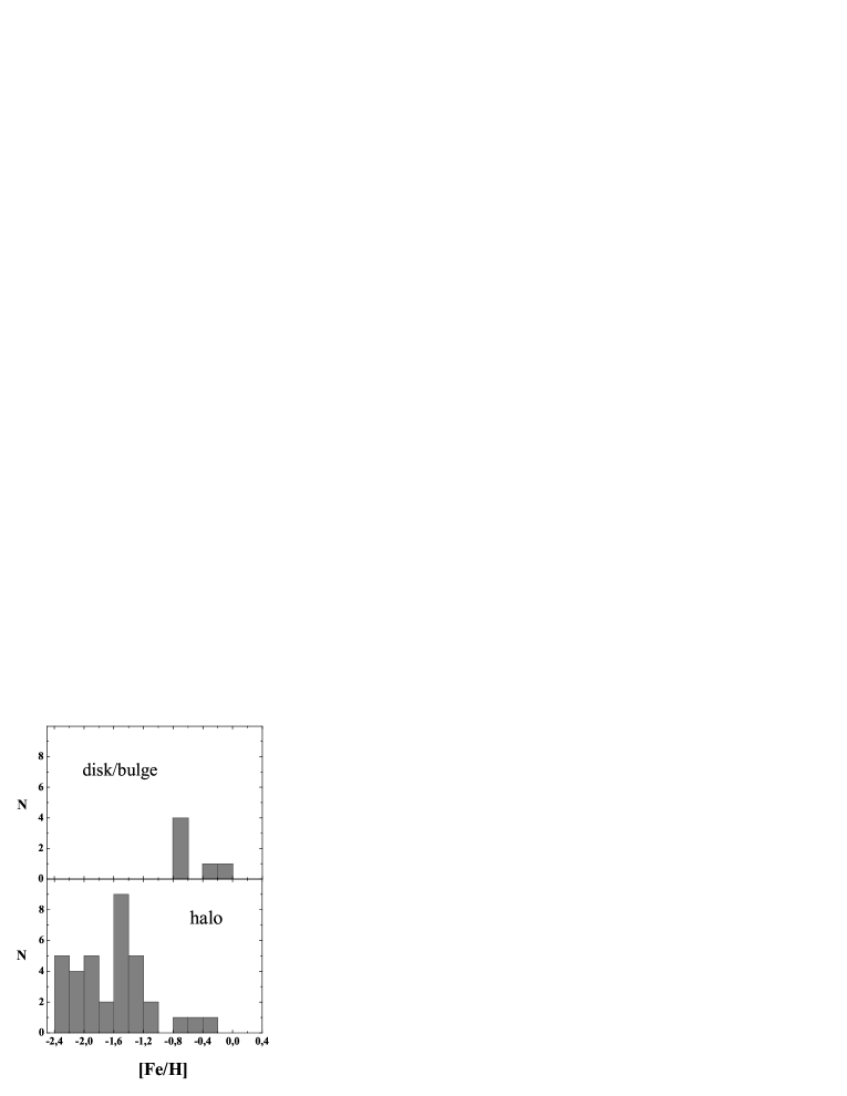
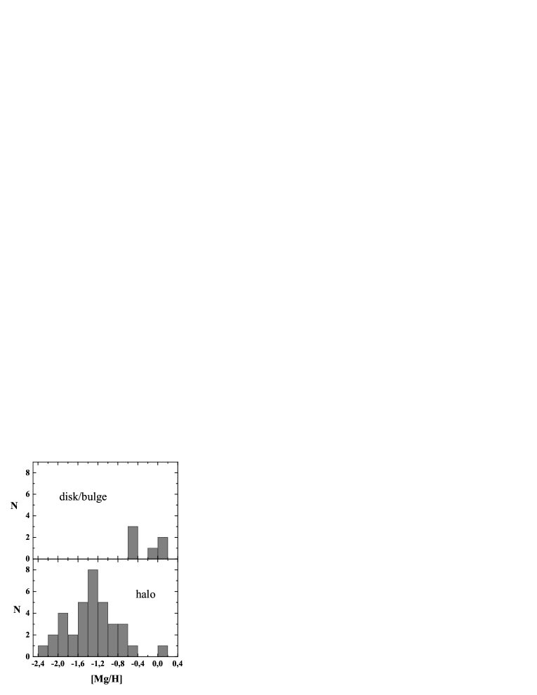
Figure 4: Distributions of iron (left-hand) and magnesium (right-hand) abundances in GCs built using the data from Pritzl et al. (2005) for objects in the two subsystems of the Galaxy: halo and disc/bulge objects.

3 Statistical analysis of magnesium abundance in clouds of the circumgalactic medium

The bimodal metallicity distribution of clouds of the circumgalactic medium was for the first time established by Lehner et al. (2013). The first results of analysing the metallicity of the circumgalactic medium of galaxies located at redshifts of $\rm z<1$ were presented and it was obtained that the metallicity distribution estimated from the alpha-element abundance in twenty eight Lyman limit systems and partial Lyman limit systems is bimodal, i.e., the distribution function has two distinct peaks with the deep minimum at $\rm\mbox{[Mg/H]}\sim-0.9$. The bimodal metallicity distribution in galaxies at redshifts from one to zero means that the metal-poor and metal-rich gas did not noticeably mix during this time interval. All the clouds are located within 100 kpc from the centers of the nearest galaxies.

The paper by Wotta et al. (2016) continued these studies. Its authors analysed the magnesium abundance in the dense circumgalactic medium for galaxies with redshifts of $\rm 0.1<z<~{}1.1$. The lines of singly-ionized magnesium are strong and well-resolved, thus, this element is an exceptional indicator of metallicity, in the authors opinion. Combined with the studies of 2013, forty four optically thin systems (pLLSs) and eleven optically thicker (LLSs) have been investigated. It has been found that the metallicity distribution of pLLSs at $z<~{}1$ is bimodal, therefore, the distribution function has two distinct peaks, each of which is close to the normal distribution with a dip between them at $\rm\mbox{[Mg/H]}\sim-0.9$. In the sample observed, the maximum of the distribution function for the metal-poor group of pLLSs is at $\rm\mbox{[Mg/H]}\sim-1.58$, for the metal-rich group it is at $\rm\mbox{[Mg/H]}\sim-0.34$ (see Fig. 5, the analogue of Fig. 12 in Wotta et al. (2016)).

Fig. 6 shows the metallicity distribution of circumgalactic clouds at redshifts of $z<1$ for the whole sample pLLSs+LLSs ($16.1<logN_{HI}<17.7$). The metallicity distribution function is bimodal with the distinct minimum at $\mbox{[Mg/H]}\sim-0.9$. Table 2 gives the number of clouds in each subgroup, the average abundance of magnesium, and the root-mean-square deviations.

The average abundance of magnesium in the sample of clouds consisting of pLLSs$+$LLSs in the metal-poor group is $\rm\mbox{[Mg/H]}=-1.49$, in the metal-rich group – $\rm\mbox{[Mg/H]}=-0.38$. Comparing the magnesium abundance in the metal-poor and metal-rich subgroups of circumgalactic clouds and the magnesium abundance in the same subgroups of GCs, one can conclude that they coincide within errors of abundance measurements in clouds of 0.3 dex. For the metal-rich group, the magnesium abundance in clouds is by 0.14 dex smaller than in GCs. For the metal-poor subgroup, the magnesium abundance in clouds is by 0.18 dex smaller than in GCs. Hence, one can assume that pLLSs+LLSs clouds can be the rest of parent clouds of GCs. It is shown in the paper by Lehner et al. (2016) that high-metallicity pLLSs$+$LLSs appear starting from $z\sim 2.5$ that corresponds to the time of their formation $T\sim 11$ Gyr ago. At redshifts of $2.5<z<3.3$, the metallicity distribution for clouds is presented mainly by a metal-poor component. It follows herefrom that, heavier-element enrichment of the fraction of metal-poor gas has taken place through thermonuclear fusion products of supernovae of the first GC generation entering into it. The second generation has subsequently been formed from this enriched gas. It should be noted that the ages of some high-metallicity Galactic GCs were estimated to be 12-13 Gyr (see Table 1 in Chattopadhyay et al. (2012)), i.e., they are as old as low-metallicity GCs according to these data. The errors of absolute age determination are large and can reach 25%. It is not excluded that the process of star cluster formation was extended in time, and low-metallicity GCs continued to form at the same time, when high-metallicity GCs originated in other clouds. The picture is complicated by the fact that the expanding shells from supernovae that have exploded in low-metallicity GCs are fragmented due to enhanced gaseous instabilities (de Avillez & Mac Low, 2002; Dedikov & Shchekinov, 2004; Vasiliev et al., 2009) and radiation losses (Vasiliev et al., 2017) in high-metallicity and low-metallicity regions. The characteristic time of metal mixing between such fragments is hundreds millions of years (de Avillez & Mac Low, 2002), which is much greater than the typical time-scale of a star-forming burst which is about several million years. Therefore, it is impossible to completely exclude the formation of low-metallicity GCs at the second stage of star formation in the clouds. It is difficult to reconstruct the exact evolutionary scenario due to age determination uncertainties.

4 Estimation of magnesium production by supernovae in the first generation of globular clusters and enrichment of the parent cloud with metals

Figure 5: Magnesium abundance distribution in 44 partial Lyman limit systems at redshifts of $0.1<~{}z<~{}1.1$ determined in Wotta et al. (2016). The metallicity distribution is bimodal. The distinct dip in the distribution is observed at [Mg/H]=-0.9.

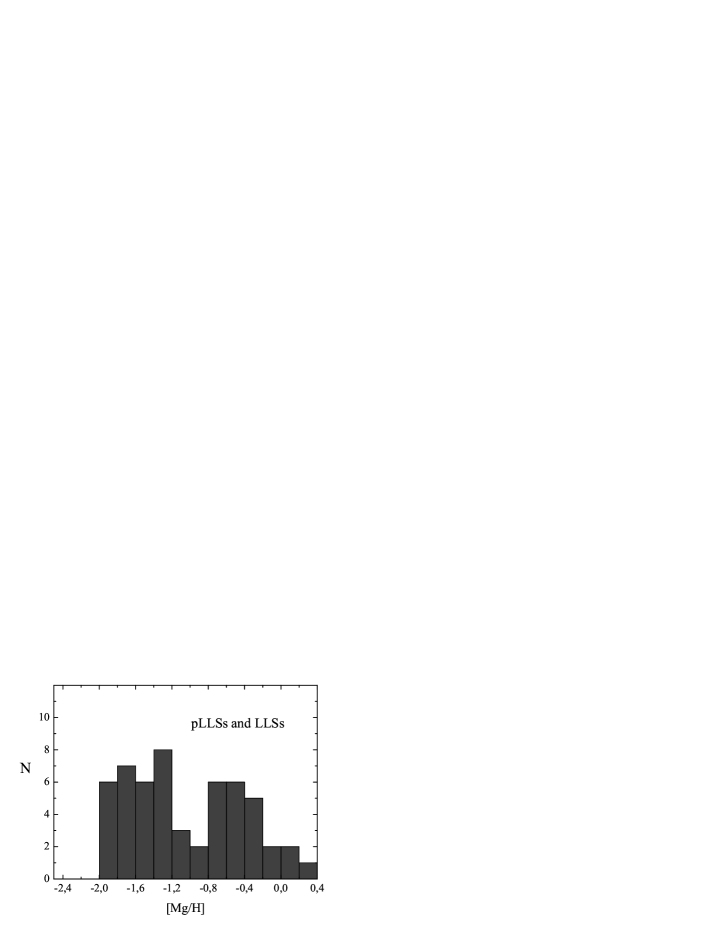
Figure 6: Magnesium abundance distribution in 55 partial Lyman limit systems and Lyman limit systems at redshifts of $0.1<~{}z<~{}1.1$ determined in Wotta et al. (2016). The metallicity distribution is bimodal. The distinct dip in the distribution is observed at [Mg/H]=-0.9.

Let us estimate the mass fraction of magnesium corresponding to the average values of [Mg/H] for metal-rich and metal-poor groups of GCs and circumgalactic clouds.

Let $Z_{Mg}$ denote the mass fraction of magnesium in relation to hydrogen in the object under study, $Z_{Mg_{\sun}}$ is the same mass fraction in the Sun. [Mg/H] can mean both the fraction by the number of atoms $N_{Mg}\over N_{H}$ and by the mass, where the mass fraction is determined with the expression $\rm N_{Mg}\cdot m_{Mg}\over N_{H}\cdot m_{H}$, with the ratio of masses of magnesium and hydrogen atoms decreasing with the logarithm difference: $\rm\mbox{[Mg/H]}=lgZ_{Mg}-lgZ_{Mg_{\sun}}$. It follows from here that $Z_{Mg}=10^{lgZ_{Mg_{\sun}}+\mbox{[Mg/H]}}$.

The mass fraction of magnesium in the Sun $Z_{Mg_{\sun}}={{N_{Mg}\cdot m_{Mg}}\over{{N_{H}\cdot m_{H}}}}X$, where $X=0.7381$ is the mass fraction of hydrogen in the Sun (Asplund et al., 2009). It follows from here that $lgZ_{Mg_{\sun}}=lg({N_{Mg}\over N_{H}})+lg({m_{Mg}\over m_{H}})+lg(X)=-3.1$. (We used the value determined in the paper by Asplund et al. (2009) for the Sun $A_{Mg}=lg({N_{Mg}\over N_{H}})+12=7.64$ ). Thus, if the magnesium abundance in GCs is $\mbox{[Mg/H]}=-1.31$, then the mass fraction of magnesium in it is $Z_{Mg}=10^{-1.31-3.1}=10^{-4.41}$. If the magnesium abundance in GCs is $\mbox{[Mg/H]}=-0.24$, then the mass fraction of magnesium in it is $Z_{Mg}=10^{-0.24-3.1}=10^{-3.34}$ Therefore, the magnesium abundance in the metal-rich GC group is twelve times higher than that in the metal-poor group.

Similar reasoning is correct for circumgalactic gaseous clouds also. The mass fraction of magnesium in the metal-rich group equals $Z_{Mg}=10^{-0.38-3.1}=10^{-3.48}$, in the metal-poor group $Z_{Mg}=10^{-1.49-3.1}=10^{-4.59}$. In the metal-rich group of circumgalactic clouds, the magnesium abundance is approximately thirteen times higher than that in the metal-poor one.

Thus, taking into consideration the similarity of metallicity distributions of GCs and circumgalactic clouds for $z<1$ and the prevalence of the metal-poor component for $z>2$, we can suppose that the metal-rich component originated from the metal-poor one through formation of GCs with subsequent enrichment with supernovae explosion products.

4.1 Limitations imposed by GCs on magnesium and iron nucleosynthesis

In the papers by Kruijssen (2014) and Shapiro et al. (2010), it is shown that the regions of gas concentration observed at high redshifts around large galaxies with the characteristic sizes of 1-3 kpc and masses $M\propto 10^{8}-10^{9}M_{\sun}$ can be the birthplaces of several hundreds of GCs, only a dozen of which have survived till our days. For their part, Lehner et al. (2013), having qualitatively estimated the properties of circumgalactic clouds, drew the conclusion that their sizes could reach several kpc.

As was shown in the paper by Ferrara et al. (2000), the process of gas enrichment with supernova explosions occurs in two stages. Supernova bursts push chemical elements out of GCs or UCDs. The expanding shells lose energy due to the high pressure of the surrounding gas and form bubbles of a relatively small size. Modelling of shell expansion is illustrated, for example, in Shen et al. (2014) and Vasiliev et al. (2017). At the second stage, metals are diffused over long distances comparable to the distance between galaxies. As it was shown by Ferrara et al. (2000), turbulent mixing of gaseous layers at the interface between shock waves from supernova can be important for determining the spatial structure of the metal distribution. The areas enriched with metals gradually increase in number and size. Unfortunately, the details of this process are not yet clear. Thus, now we observe the relics of the primeval clouds which served as the building material for metal-poor GCs, and the remains of the metal-enriched parts of these clouds, from which the high-metallicity GC group was formed.

It was shown by Lehner et al. (2013) that for the metal-poor sample of pLLSs and LLSs the number of hydrogen atoms along the line of sight $logN_{H}=19.0\pm 0.5$, while for the metal-rich sample $logN_{H}=18.6\pm 0.7$. The sizes and covering factors are similar. Therefore, the metal-enriched gas in the circumgalactic medium may be on average less massive than the metal-poor gas by a factor of $\sim 2$ (Lehner et al., 2013).

Let us estimate the number of supernovae capable to enrich half the mass of the primeval cloud up to the observed abundances of chemical elements. If the mass of a cloud $M\approx 10^{9}M_{\sun}$, then the magnesium mass in the metal-poor cloud $M_{Mg}=10^{9-3.1-1.49}=10^{4.41}M_{\sun}$. Taking into account that the mass of the metal-rich cloud is twice smaller $M\approx 10^{8.7}M_{\sun}$, the mass of Mg in it is $M_{Mg}=10^{8.7-3.1-0.38}=10^{5.22}M_{\sun}$. If we assume that a metal-rich cloud with $\mbox{[Mg/H]}=-0.38$ has been formed from a metal-poor one with $\mbox{[Mg/H]}=-1.49$, then the cloud has acquired $M_{Mg}\approx 10^{5.2}M_{\sun}$.

It is natural to expect that the major contribution in magnesium production has been made by rapidly evolving massive stars that exploded as SNe CC . According to calculations of Tsujimoto et al. (1995) and Hirschi et al. (2005), a single core-collapse supernova ejects $M_{Mg}\approx 0.1M_{\sun}$ when exploding. In order to produce $M_{Mg}\approx 10^{5.2}M_{\sun}$, $10^{6.2}$ SNe CC are necessary. For the reasoning given, the accepted mass of a cloud is not critical, since both the magnesium mass in the cloud and the number of supernovae in it are proportional to the mass of the cloud: the cloud with $M\approx 10^{8}M_{\sun}$ will obtain the magnesium mass $M_{Mg}\approx 10^{4.2}M_{\sun}$ with $10^{5.2}$ SNe CC required.

Let us estimate whether it is possible to expect such a number of SNe CC resulting from star formation. As is shown in the paper by Shapiro et al. (2010) (and references therein), structures with a mass of $10^{-6}-10^{-3}$ of the gaseous clouds mass have been formed inside it at the initial stages of evolution of a galaxy; and, what is actually important for our study, about 10% of the mass of a cloud is transferred to stars (Wilson et al., 2003), from which the first generation of GCs can later develop. Namely, the mass of stars formed from a cloud with $M\propto 10^{9}M_{\sun}$ will be $M_{*}\propto 10^{8}M_{\sun}$.

The stellar mass distribution is described by the initial mass function (IMF). The IMF is conventionally denoted as $\varphi(m)$ and determined in such a way that the mass fraction of stars enclosed in the interval [$m;m+dm$] is described with the expression $m\varphi(m)dm$. The integral $\!\!\int_{m_{l}}^{m_{u}}\!\!m\varphi(m)dm=1$ is a condition of IMF normalizing, where $m_{l}$, the minimum mass of forming stars, is assumed to be equal to $0.1M_{\sun}$, $m_{u}$ – the maximum mass of forming stars is assumed to be equal to $70M_{\sun}$.

We are interested in stars that can explode as SNe CC. Such stars have an initial mass of greater than $8M_{\sun}$.

It was found in recent papers (Weisz et al., 2015) (and references therein) that the high-mass IMF slope ($m>1.5M_{\sun}$) inferred from numerous studies of young star clusters is in the range of 1.2$\div$1.7. The IMF slope is constant and equal to 1.35 in case if we choose the Salpeter IMF (Salpeter, 1955). Weisz et al. (2015) concluded that for 85 star clusters in M31 the high-mass slope is universal and equal to $1.45^{+0.03}_{-0.06}$. It is difficult to use the findings of Weisz et al. (2015); Kroupa (2001, 2003) and Zhang & Fall (1999) in our calculations, because the normalization coefficients are not given. For the multi-slope expression of IMF, the normalization coefficients may be different for various mass ranges, as it is shown in Kroupa et al. (1993) and (1986). Therefore, in the following we will use the IMF shape proposed by Salpeter (1955). Let us recall that it was defined while studying young star clusters: $\varphi(m)=0.1716\cdot m^{-2.35}$. Note, however, that differences between the results of our calculations using the mentioned various IMF slopes are within 5%.

Let us estimate the stellar mass fraction that is accounted for by SNe CC: $\!\!\int_{8}^{70}\!\!m\varphi(m)dm\approx 0.12$. There are studies (Acharova et al., 2013; Kochanek et al., 2008) showing that the maximum mass of stars resulting in SNe CC can not exceed $30M_{\sun}$. In this case, only $\!\!\int_{8}^{30}\!\!m\varphi(m)dm\approx 0.09$ of the GC mass is accounted for by SNe CC. Thus, about 10% of GC mass is accounted for by SNe CC in two considered cases. Consequently, it can be concluded that the mass of supernovae formed from a cloud with $M\propto 10^{9}M_{\sun}$ will be $M_{*}\approx 10^{7}M_{\sun}$.

The average mass of a star that explodes as a supernova is found from formula (1) from Tsujimoto et al. (1995):

$\langle Mcc\rangle={{\!\!\int_{8}^{70}\!\!m\varphi(m)dm}\over{\!\!\int_{8}^{70}\!\!\varphi(m)dm}}\approx 17.5$ $M_{\sun}$ ($\langle Mcc\rangle=15M_{\sun}$ for $m_{u}=30M_{\sun}$).

It follows from here that approximately $10^{5.8}$ SNe CC can explode in the cloud, which is 2.5 times smaller than the required number of supernovae for the thirteen times enrichment of one half of the cloud with magnesium. Such an amount of SNe CC will generate $M_{Mg}\approx 10^{4.8}M_{\sun}$.

Three possibilities to solve the issue of producing the necessary mass of magnesium can be seen. The first one is the following: the fraction of gas in the cloud enriched by the products of first supernovae constitutes not 50% but 20% ($M\approx 10^{8.3}M_{\sun}$) of the initial cloud mass. This assumption looks believable taking into account the errors of measuring $logN_{H}$ (Lehner et al., 2013). Then the mass of magnesium in the enriched part of the cloud will be $M_{Mg}=10^{8.3-3.1-0.38}=10^{4.82}M_{\sun}$. The second possibility is that the fraction of the cloud gas transformed into stars should be about 25%. This is much, at first glance, but as is shown in the papers by Kennicutt & Evans (2012) (and references therein) and Wu et al. (2009), it is observationally established that at a surface density of $100-300M_{\sun}/$pc² a so-called explosive star-formation mode occurs, in which the fraction of gas transformed into stars can exceed 50%. Theoretical studies confirm such a possibility (Mouschovias & Spitzer, 1976; McKee, 1989). The third possibility is the production of the residuary amount of magnesium by another type of supernovae, SNe Ia. According to available models, in which SNe Ia is considered the result of a white dwarf explosion, the magnesium mass emitted during the explosion is approximately equal to $M_{Mg}\approx 0.01M_{\sun}$ (Tsujimoto et al., 1995). Therefore, to produce the missing $M_{Mg}\approx 10^{5}M_{\sun}$, the number of SNe Ia should be 6 times higher than the number of SNe CC. Before omitting this alternative, let us consider the analysis of the iron abundance in GCs, since SNe Ia are thought to be the main supplier of iron.

4.2 Analysis of the enrichment of globular clusters with iron

In a similar way as conducted for magnesium, we will analyse the iron abundance in GCs. Since there is no data on the iron abundance in circumgalactic clouds, then the conclusions about the iron abundance in GCs are generalized to the iron abundance in the gaseous medium from which they have been formed. Let us denote $Z_{Fe}$ – the iron mass fraction in relation to hydrogen in the objects under study, $Z_{{Fe}_{\sun}}$ is the iron mass fraction in the Sun. It follows that $\rm Z_{Fe}=10^{lgZ_{{Fe}_{\sun}}+[Fe/H]}$.

The mass fraction of iron in the Sun $Z_{Fe_{\sun}}={{N_{Fe}\cdot m_{Fe}}\over{{N_{H}\cdot m_{H}}}}X$, where $X=0.7381$ is the hydrogen mass fraction in the Sun (Asplund et al., 2009). Hence, $lgZ_{Fe_{\sun}}=lg({N_{Fe}\over N_{H}})+lg({m_{Fe}\over m_{H}})+lg(X)=-2.84$ (We used the value defined in the paper of Asplund et al. (2009) for the Sun $A_{Fe}=lg({N_{Fe}\over N_{H}})+12=7.54$). Thus, if the iron abundance in a GC $\mbox{[Fe/H]}=-1.66$, then the iron mass fraction in it $Z_{Fe}=10^{-1.66-2.84}=10^{-4.50}$. If the iron abundance in a GC $\mbox{[Fe/H]}=-0.47$, then the iron mass fraction in it $Z_{Fe}=10^{-0.47-2.84}=10^{-3.31}$. In other words, the iron abundance in the metal-rich GC group is fifteen times higher than that in the metal-poor. Now we assume that the iron mass fraction in the clouds is the same as in GCs. If the mass of a cloud $M\approx 10^{9}M_{\sun}$, then the iron mass $M_{Fe}\approx 10^{4.5}M_{\sun}$ in the metal-poor cloud.

Let us, first, consider the case when the fraction of the enriched part of the cloud is 20% of the initial cloud mass (first possibility formulated in Sec. 4.1). Then the iron mass has increased from $M_{Fe}=10^{8.3-4.5}=10^{3.8}M_{\sun}$ to $M_{Fe}=10^{8.3-3.31}\approx 10^{5}M_{\sun}$, and the cloud gained $M_{Fe}=10^{4.97}\approx 10^{5}M_{\sun}$.

When a core-collapse supernova explodes, $M_{Fe}\approx 0.01M_{\sun}$ is emitted (Tsujimoto et al., 1995). Hence, $10^{5.8}$ SNe CC will produce $M_{Fe}=10^{3.8}M_{\sun}$. Thus, the contribution of core-collapse supernovae to the production of iron is negligibly small. Consequently, $M_{Fe}\approx 10^{5}M_{\sun}$ should be produced by other sources – SNe Ia, and mainly by those formed from short-lived progenitors – prompt SNe Ia (pSNe Ia), since according to Mannucci et al. (2006), Li et al. (2011), Maoz et al. (2014), Rodney et al. (2014), and Andersen & Hjorth (2018), SNe Ia evolved from long-lived progenitors have not been observed for initial 1-1.5 Gyr. If we assume that the canonically accepted $0.6M_{\sun}$ of iron is emitted with the explosion of such a pSNe Ia (Nomoto, 1997), then $10^{5.2}$ of pSNe Ia will be necessary which is four times smaller than SNe CC. If we assume that with the pSNe Ia explosion, $0.23M_{\sun}$ of iron is emitted (it is the mass gained according to theoretical calculations conducted in Acharova et al. (2013) for pSNe Ia and complying with the estimate of the nickel mass emitted in explosions of some SNe Ia (Childress et al., 2015)), then $10^{5.6}$ of pSNe Ia will be needed which is 1.6 times smaller than the number of SNe CC. For comparison, according to Li et al. (2011), the current frequency of explosions of SNe CC in our Galaxy equals 2.3 per century, and the frequency of bursts of pSNe Ia in star-forming regions is 0.43 per century. In other words, in massive galaxies, the frequency of bursts of SNe CC is five times higher than those of pSNe Ia. It is important to note that the conclusions on the frequency of supernovae explosions in Li et al. (2011) were drawn from the analysis of evolved galaxies close to the modern age. We, however, are concerned with the GCs, in which the relation between the supernovae subtypes is not measured observationally. The characteristic property of GCs is in the fact that the density of stars is high in them. When analysing the obtained results, we conclude, that our first assumption leads to the reliable estimates of the frequencies of SNe CC and pSNe Ia bursts and could take place in reality.

We now turn to the second possibility, formulated in Sec. 4.1: the mass of the enriched part of the cloud is twice less than the original one and fraction of the cloud gas transformed into stars should be $\sim 25\%$. In this case, the mass of iron in the enriched part of the cloud is $M_{Fe}=10^{5.4}M_{\sun}$. It can be accepted that the cloud gained $M_{Fe}=10^{5.37}M_{\sun}$. The contribution to the iron production by $10^{6.2}$ SNe CC is negligible, as it was argued above. Consequently, when producing $0.6M_{\sun}$ of iron by a single supernova, the necessary number of pSNe Ia is $10^{5.6}$ which is four times smaller than the number of SNe CC. On the other hand, when producing $0.23M_{\sun}$ of iron by a single supernova, the necessary number of pSNe Ia is $10^{6}$, which is $1.6$ times less than the number of SNe CC. According to the presented analysis of the frequencies of SNe CC and pSNe Ia explosions, the ratio of frequencies has not changed with respect to the first considered possibility. One may conclude that the second cloud enrichment scenario is probable.

From the above arguments, it follows automatically that the third possibility formulated in Sec. 4.1 is impossible, because a number of pSNe Ia cannot six times exceed a number of SNe CC.

Can restrictions be placed on the frequency of different types of supernovae from analysing of other properties of globular clusters? It is the characteristic feature of GCs that the density of stars is high in them and stellar collisions are possible (Hills & Day, 1976; Fregeau et al., 2004). Some researchers consider blue straggler stars to be an observational manifestation of such processes (Ferraro et al., 2009; Dalessandro et al., 2013; Simunovic et al., 2014; Li et al., 2018). It is important to notice that the exact nature of stars that produce SNe Ia, remains unknown (Ruiter et al., 2011; Hillebrandt & Niemeyer, 2000; Leibundgut, 2000). It is generally agreed that type SNe Ia is caused by an explosion of a carbon-oxygen white dwarf. However, the details of the process of accretion of companions matter onto it remain unclear (Yungelson, 2008). At the same time, the recent finding by Sana et al. (2012) shows that the binary interaction may affect 70% or more of the massive star population. This result is confirmed by the studies of Kobulnicky & Fryer (2007). At the same time, the interaction of binary stars is considered to be an important formation channel of SN Ibc supernovae also (Nomoto, 1995), whose spectra show the high magnesium abundance and the low iron abundance (Smartt, 2009). Thus, it can be concluded that the available data, unfortunately, are not enough to predict the ratio of the SNe CC and pSNe Ia frequencies. Analysis of abundances of chemical elements is the only source of information about the number of different types of supernovae in GCs.

5 Conclusions

We have conducted a statistical study of the iron and magnesium abundances in GCs circumgalactic gaseous clouds. On the comparison between the magnesium abundance in the metal-poor and metal-rich subgroups of circumstellar clouds at redshifts of $0.1<z<1.1$ with magnesium and the magnesium abundance in similar subgroups of GCs, we can conclude that they coincide within an error of abundance measurements in clouds of 0.3 dex. The magnesium abundance in clouds is by 0.14 dex smaller than in GCs for the metal-rich subgroup and by 0.18 dex – for the metal-poor subgroup. An assumption can be made from this that the pLLSs+LLSs clouds are the remnants of host clouds of GCs.

From the fact that the cloud metallicity distribution is presented only by the metal-poor component at redshifts $2.5<z<3.3$, it follows that the fraction of metal-poor gas was enriched with heavier elements through thermonuclear fusion products of supernovae of the first GC generation entering into it. The second generation of GCs was formed from this enriched gas.

Let us discuss how the scheme proposed in our study agrees with ideas developed in the literature. In the literature, the process of formation of globular clusters is considered within the framework of two basic concepts. According to the first one, metal-poor GCs are formed in low-mass galaxies and then, together with parent galaxies, are accreted to the halo of massive galaxies (Searl & Zinn (1978), Shapiro et al. (2010) and references therein). Metal-rich GCs form from the gas enriched by stars of massive galaxies. These stars were not constituents of metal-poor GCs (see also Elmegreen et al. (2012)). According to the second concept, the halo of each massive galaxy experiences two episodes of the GC formation (the ‘in situ’ model) (Forbes, Brodie & Grillmair, 1997). First, when a proto-galactic cloud collapses, low-metallicity GCs are formed. High-metallicity GCs originate during the second stage of star formation.

The results of our study are consistent with the second aforementioned concept (Forbes, Brodie & Grillmair, 1997).

Our reasoning can be relevant not only for GCs but also in the case of ultra-compact dwarf galaxies (UCDs), because the last ones have metallicities, spatial distribution and specific frequencies similar to those of GCs (e.g. Zhang et al. (2016), Voggel et al. (2016), Mieske et al. (2012), Francis et al. (2012) and references in these papers). UCDs are more massive, luminous, and have higher mass-to-light ratios than globular clusters but are fainter and more compact than dwarf elliptical galaxies and M32-like galaxies. It was proposed many times in the literature that UCDs and GCs were formed under similar conditions (Goodman & Bekki (2018), Romanowsky et al. (2017), Goerdt et al. (2008) Chattopadhyay et al. (2012) and references in these papers).

Unfortunately, the available literature data about the properties of pLLSs are not sufficient to make definite conclusions concerning the spatial distribution of their low-metallicity and high-metallicity representatives relative to the planes of galactic disks. It is clear that DLAs ($logN_{HI}>20.3$) are more concentrated to the planes of galactic disks. The typical distances from host galactic planes for DLAs are comparable with these of thick disk objects in our Galaxy (Rao et al., 2011). DLAs are on average denser than pLLSs. The mean metallicity of DLAs is close to the metallicity of high-metallicity pLLSs. We cannot extrapolate our conclusions to DLAs, because there are no enough data in the literature for the statistical analysis of magnesium abundances in them (e.g. Vladilo et al. (2011)).

Studying the abundances of chemical elements in GCs, one can come to nontrivial conclusions regarding the fraction of gas transformed into stars, the contribution of supernovae to the production of heavier elements and the fraction of the circumgalactic gas enriched in chemical elements synthesized in it during first starforming bursts. The amount of magnesium produced by first generations of GCs does agree with two hypotheses: i) the fraction of mass of the enriched part of the cloud is $20\%$ of the initial cloud mass and the fraction of the cloud gas, transformed into stars is $10\%$; ii) the mass of the enriched part of the cloud is twice less than the original one, and the fraction of the cloud gas transformed into stars is $25\%$.

According to the available observations and theoretical calculations, SNe CC produce a negligible amount of iron. The bulk of its mass is produced by SNe Ia, and namely by those the progenitors of which explode in the first Myr after forming. It is shown in the present study that the number of pSNe Ia in GCs must be 2-4 times less than the number of SNe CC.

References

- Acharova et al. (2013) Acharova I.A. , Gibson B.K. , Mishurov Yu. N. , et al., 2013, A&A, 557, 107
- Andersen & Hjorth (2018) Andersen P. and Hjorth J., 2018, 2018arXiv180100793A
- Asplund et al. (2009) Asplund M., Grevesse N., Sauval A.J.,et al. 2009, ARA&A, 47, 481
- de Avillez & Mac Low (2002) de Avillez M.A., Mac Low M.-M., 2002, ApJ, 581, 1047
- Brandt et al. (2010) Brandt T. D., Tojeiro R., Aubourg E., et al. 2010, AJ, 140, 804
- Carretta et al. (2010) Carretta E., Bragaglia A., Gratton R. G, 2010, A&A, 516, A55
- Chattopadhyay et al. (2012) Chattopadhyay T., Sharina M., Davoust E., et al. 2012, ApJ, 750, 91
- Childress et al. (2015) Childress M.J., Hillier D.J., Seitenzahl I., et al. 2015, MNRAS, 454, 3816
- Dahlen et al. (2004) Dahlen T. et al. 2004, ApJ, 613, 189
- Dalessandro et al. (2013) Dalessandro E., Ferraro F. R., Massari D., et al. 2013, ApJ, 778, 135
- Dedikov & Shchekinov (2004) Dedikov S.Yu., Shchekinov Yu.A., 2004, Astronomy Reports, 48, 9
- Dias et al. (2016) Dias B., Barbuy B., Saviane I., et al., 2016, A&A, 590, 9
- Elmegreen et al. (2012) Elmegreen B.G., Malhotra S., Rhoads J., 2012, ApJ, 757, 9
- Ferrara et al. (2000) Ferrara A., Pettini M. & Shchekinov Yu., 2000, MNRAS, 319, 539
- Ferraro et al. (2009) Ferraro F. R., Beccari G., Dalessandro E., et al. 2009, Nature, 462, 1028
- Forbes, Brodie & Grillmair (1997) Forbes D. A., Brodie J. P., Grillmair C. J., 1997, AJ, 113, 1652
- Francis et al. (2012) Francis K. J., Drinkwater M. J., Chilingarian I. V., Bolt A. M., Firth P., 2012, MNRAS, 425, 325
- Fregeau et al. (2004) Fregeau J. M., Cheung P., Portegies Zwart S. F.,& Rasio F. A., 2004, MNRAS, 352, 1
- Goerdt et al. (2008) Goerdt T., Moore B., Kazantzidis S., Kaufmann T., Maccio A., Stadel J., 2008, MNRAS, 385, 2136
- Goodman & Bekki (2018) Goodman M. & Bekki K., 2018, MNRAS 478, 3564
- Harris (1996) Harris W. E., 1996, AJ, 112, 1487
- Hillebrandt & Niemeyer (2000) Hillebrandt W., Niemeyer J.C., 2000, ARA&A, 38, 191
- Hills & Day (1976) Hills J. G. & Day C.A., 1976, ApL, 17, 87
- Hirschi et al. (2005) Hirschi R., Meynet G., Maeder A. 2005, A&A, 433, 1013
- Kennicutt & Evans (2012) Kennicutt R.C., Evans N.J., 2012, ARA&A, 50, 531
- Kobulnicky & Fryer (2007) Kobulnicky H.A., Fryer C.L., 2007, ApJ, 670, 747
- Kochanek et al. (2008) Kochanek C., Beacom J., Kistler M., et al. 2008, ApJ, 684, 1336
- Kruijssen (2014) Kruijssen J. M. Diederik, 2014 Classical and Quantum Gravity, 31, Issue 24, article id. 244006
- Kroupa et al. (1993) Kroupa P., Tout C. A., & Gilmore G. 1993, MNRAS, 262, 545
- Kroupa (2001) Kroupa P. 2001, MNRAS, 322, 231
- Kroupa (2003) Kroupa P., & Weidner C. 2003, ApJ, 598, 1076
- Lehner et al. (2016) Lehner N., O’Meara J.M., Howk J.C., 2016, ApJ, 833, L283
- Lehner et al. (2013) Lehner N., Howk J. C., Tripp T. M., et al. 2013, ApJ, 770, 138
- Li et al. (2011) Li W., Chornock R., Leaman J., et al. 2011, MNRAS, 412, L1473
- Li et al. (2018) Li C., Deng L., de Grijs R., Jiang D., Xin Y. 2018, ApJ, 856, L25
- Leibundgut (2000) Leibundgut B., 2000, A&ARv, 10, 179
- Limongi & Chieffi (2003) Limongi M., Chieffi A. 2003, ApJ, 592, 404
- Mackey & Gilmore (2004) Mackey A. D., Gilmore G. F. 2004, MNRAS, 355, 504
- Mannucci et al. (2006) Mannucci F. , Della Valle M. and Panagia N. 2006, MNRAS, 370, 773
- Maoz et al. (2014) Maoz D., Mannucci F., Nelemans G., 2014, ARA&A, 52, 107
- Marin-Franch et al. (2009) Marin-Franch A., Aparicio A., Piotto G.et al., 2009, ApJ, 694, 1498
- Marsakov & Suchkov (1977) Marsakov V.A., Suchkov A.A., 1997, SvA, 21, 700
- McKee (1989) McKee C. F. 1989, ApJ, 345, 782
- Mieske et al. (2012) Mieske S., Hilker M., Misgeld I., 2012, A&A, 537, 3
- Mouschovias & Spitzer (1976) Mouschovias T.Ch., Spitzer L.Jr. 1976, ApJ, 210, 326
- Nomoto (1997) Nomoto K., Iwamoto K., Nakasato N., et al. 1997, Nucl. Phys. A, 621, 467
- Nomoto (1995) Nomoto K., Iwamoto K., Suzuki T., 1995, Phys. Rep., 256, 173
- Pritzl et al. (2005) Pritzl B.J., Venn K.A., Irwin M., 2005, AJ, 130, 2140
- Rao et al. (2011) Rao S.M., Belfort-Mihalyi M., Turnshek D.A., et al., 2011, MNRAS, 416, 1215
- Rodney et al. (2014) Rodney S. A., Riess A., Strogler L.-G. 2014, AJ, 148, 13
- Romanowsky et al. (2017) Romanowsky A., Brodie J. P. and SAGES Collaboration, 2017, in C. Charbonnel & A. Nota, eds., Proc. IAU Sympo. 316: Formation, Evolution, and Survival of Massive Star Clusters. Cambridge Univ. Press, Cambridge, p. 105
- Ruiter et al. (2011) Ruiter A. J., Belczynski K., Sim S. A., et al. 2011, MNRAS, 417, 408
- Salpeter (1955) Salpeter E. E., 1955, ApJ, 121, 161
- Sana et al. (2012) Sana H., de Mink S. E., de Koter A., et al. 2012, Science, 337, 444
- (55) Scalo J. M., 1986, FCPh, 11, 1
- Searl & Zinn (1978) Searle L. & Zinn R., 1978, ApJ, 225, 357
- Shapiro et al. (2010) Shapiro K.L., Genzel R., Forster S. 2010 MNRAS, 403, L36
- Shen et al. (2014) Shen S., Madau P., Conroy C., et al., 2014, ApJ, 792, 99
- Simunovic et al. (2014) Simunovic M., Puzia T. H. & Sills A. 2014, ApJ, 795, L10
- Smartt (2009) Smartt S. J., 2009, ARA&A, 47, 63
- Strolger et al. (2005) Strolger L.-G., et al, 2005, ApJ, 635, 1370
- Tsujimoto et al. (1995) Tsujimoto, T., Nomoto, K., Yoshii, Y., et al. 1995, MNRAS, 277, 945
- Wilson et al. (2003) Wilson C. D., Scoville N., Madden S. C., Charmandaris V., 2003, ApJ, 599, 1049
- Yungelson (2008) Yungelson L. R., 2008, Astronomy Letters, 34, 620
- VandenBerg et al. (2013) VandenBerg Don A., Brogaard K., Leaman R., Casagrande L., 2013, ApJ 775, 134
- Vasiliev et al. (2017) Vasiliev E. O., Shchekinov Y., Nath B., 2017, MNRAS, 468, 2757
- Vasiliev et al. (2009) Vasiliev E.O., Dedikov S.Yu., Shchekinov Yu.A., 2009, AstBu, 64,317
- Vladilo et al. (2011) Vladilo G., Abate C., Yin J., Cescutti G., Matteucci F., 2011, A&A, 530, 33
- Voggel et al. (2016) Voggel K.; Hilker M.; Richtler T., 2016, A&A, 586, 102
- Weisz et al. (2015) Weisz D.R., Johnson L.C., Foreman-Mackey D., 2015, ApJ, 806, 198
- Woosley & Weaver (1995) Woosley S., Weaver T. 1995, ApJS, 101, 181
- Wotta et al. (2016) Wotta C.B., Lehner N., Howk J.C.,et al. 2016, ApJ,831,95
- Wu et al. (2009) Wu J., Vanden Bout P.A., Evans N.J., et al. 2009, ApJ, 707, 988
- Zhang et al. (2016) Zhang H.-X. et al. 2018, ApJ, 858, 37
- Zhang & Fall (1999) Zhang Q.,& Fall S.M. 1999, ApJ, 527, 81
- Zinn (1985) Zinn R. 1985, ApJ, 293, 424