Adaptive Semi-supervised Learning for Cross-domain
Sentiment Classification

Abstract

We consider the cross-domain sentiment classification problem, where a sentiment classifier is to be learned from a source domain and to be generalized to a target domain. Our approach explicitly minimizes the distance between the source and the target instances in an embedded feature space. With the difference between source and target minimized, we then exploit additional information from the target domain by consolidating the idea of semi-supervised learning, for which, we jointly employ two regularizations – entropy minimization and self-ensemble bootstrapping – to incorporate the unlabeled target data for classifier refinement. Our experimental results demonstrate that the proposed approach can better leverage unlabeled data from the target domain and achieve substantial improvements over baseline methods in various experimental settings.

1 Introduction

In practice, it is often difficult and costly to annotate sufficient training data for diverse application domains on-the-fly. We may have sufficient labeled data in an existing domain (called the source domain), but very few or no labeled data in a new domain (called the target domain). This issue has motivated research on cross-domain sentiment classification, where knowledge in the source domain is transferred to the target domain in order to alleviate the required labeling effort.

One key challenge of domain adaptation is that data in the source and target domains are drawn from different distributions. Thus, adaptation performance will decline with an increase in distribution difference. Specifically, in sentiment analysis, reviews of different products have different vocabulary. For instance, restaurants reviews would contain opinion words such as “tender”, “tasty”, or “undercooked” and movie reviews would contain “thrilling”, “horrific”, or “hilarious”. The intersection between these two sets of opinion words could be small which makes domain adaptation difficult.

Several techniques have been proposed for addressing the problem of domain shifting. The aim is to bridge the source and target domains by learning domain-invariant feature representations so that a classifier trained on a source domain can be adapted to another target domain. In cross-domain sentiment classification, many works  Blitzer et al. (2007); Pan et al. (2010); Zhou et al. (2015); Wu and Huang (2016); Yu and Jiang (2016) utilize a key intuition that domain-specific features could be aligned with the help of domain-invariant features (pivot features). For instance, “hilarious” and “tasty” could be aligned as both of them are relevant to “good”.

Despite their promising results, these works share two major limitations. First, they highly depend on the heuristic selection of pivot features, which may be sensitive to different applications. Thus the learned new representations may not effectively reduce the domain difference. Furthermore, these works only utilize the unlabeled target data for representation learning while the sentiment classifier was solely trained on the source domain. There have not been many studies on exploiting unlabeled target data for refining the classifier, even though it may contain beneficial information. How to effectively leverage unlabeled target data still remains an important challenge for domain adaptation.

In this work, we argue that the information from unlabeled target data is beneficial for domain adaptation and we propose a novel Domain Adaptive Semi-supervised learning framework (DAS) to better exploit it. Our main intuition is to treat the problem as a semi-supervised learning task by considering target instances as unlabeled data, assuming the domain distance can be effectively reduced through domain-invariant representation learning. Specifically, the proposed approach jointly performs feature adaptation and semi-supervised learning in a multi-task learning setting. For feature adaptation, it explicitly minimizes the distance between the encoded representations of the two domains. On this basis, two semi-supervised regularizations – entropy minimization and self-ensemble bootstrapping – are jointly employed to exploit unlabeled target data for classifier refinement.

We evaluate our method rigorously under multiple experimental settings by taking label distribution and corpus size into consideration. The results show that our model is able to obtain significant improvements over strong baselines. We also demonstrate through a series of analysis that the proposed method benefits greatly from incorporating unlabeled target data via semi-supervised learning, which is consistent with our motivation. Our datasets and source code can be obtained from https://github.com/ruidan/DAS.

2 Related Work

Domain Adaptation: The majority of feature adaptation methods for sentiment analysis rely on a key intuition that even though certain opinion words are completely distinct for each domain, they can be aligned if they have high correlation with some domain-invariant opinion words (pivot words) such as “excellent” or “terrible”. Blitzer et al. (2007) proposed a method based on structural correspondence learning (SCL), which uses pivot feature prediction to induce a projected feature space that works well for both the source and the target domains. The pivot words are selected in a way to cover common domain-invariant opinion words. Subsequent research aims to better align the domain-specific words Pan et al. (2010); He et al. (2011); Wu and Huang (2016) such that the domain discrepancy could be reduced. More recently, Yu and Jiang (2016) borrow the idea of pivot feature prediction from SCL and extend it to a neural network-based solution with auxiliary tasks. In their experiment, substantial improvement over SCL has been observed due to the use of real-valued word embeddings. Unsupervised representation learning with deep neural networks (DNN) such as denoising autoencoders has also been explored for feature adaptation Glorot et al. (2011); Chen et al. (2012); Yang and Eisenstein (2014). It has been shown that DNNs could learn transferable representations that disentangle the underlying factors of variation behind data samples.

Although the aforementioned methods aim to reduce the domain discrepancy, they do not explicitly minimize the distance between distributions, and some of them highly rely on the selection of pivot features. In our method, we formally construct an objective for this purpose. Similar ideas have been explored in many computer vision problems, where the representations of the underlying domains are encouraged to be similar through explicit objectives Tzeng et al. (2014); Ganin and Lempitsky (2015); Long et al. (2015); Zhuang et al. (2015); Long et al. (2017) such as maximum mean discrepancy (MMD) Gretton et al. (2012). In NLP tasks, Li et al. (2017) and Chen et al. (2017) both proposed using adversarial training framework for reducing domain difference. In their model, a sub-network is added as a domain discriminator while deep features are learned to confuse the discriminator. The feature adaptation component in our model shares similar intuition with MMD and adversary training. We will show a detailed comparison with them in our experiments.

Semi-supervised Learning: We attempt to treat domain adaptation as a semi-supervised learning task by considering the target instances as unlabeled data. Some efforts have been initiated on transfer learning from unlabeled data Dai et al. (2007); Jiang and Zhai (2007); Wu et al. (2009). In our model, we reduce the domain discrepancy by feature adaptation, and thereafter adopt semi-supervised learning techniques to learn from unlabeled data. Primarily motivated by Grandvalet and Bengio (2004) and Laine and Aila (2017), we employed entropy minimization and self-ensemble bootstrapping as regularizations to incorporate unlabeled data. Our experimental results show that both methods are effective when jointly trained with the feature adaptation objective, which confirms to our motivation.

3 Model Description

3.1 Notations and Model Overview

We conduct most of our experiments under an unsupervised domain adaptation setting, where we have no labeled data from the target domain. Consider two sets $D_{s}$ and $D_{t}$. $D_{s}=\{\mathbf{x}_{i}^{(s)},\mathbf{y}_{i}^{(s)}\}|_{i=1}^{n_{s}}$ is from the source domain with $n_{s}$ labeled examples, where $\mathbf{y}_{i}\in\mathbb{R}^{C}$ is a one-hot vector representation of sentiment label and $C$ denotes the number of classes. $D_{t}=\{\mathbf{x}_{i}^{(t)}\}|_{i=1}^{n_{t}}$ is from the target domain with $n_{t}$ unlabeled examples. $N=n_{s}+n_{t}$ denotes the total number of training documents including both labeled and unlabeled. We aim to learn a sentiment classifier from $D_{s}$ and $D_{t}$ such that the classifier would work well on the target domain. We also present some results under a setting where we assume that a small number of labeled target examples are available (see Figure 3).

For the proposed model, we denote $G$ parameterized by $\theta_{g}$ as a neural-based feature encoder that maps documents from both domains to a shared feature space, and $\mathcal{F}$ parameterized by $\theta_{f}$ as a fully connected layer with softmax activation serving as the sentiment classifier. We aim to learn feature representations that are domain-invariant and at the same time discriminative on both domains, thus we simultaneously consider three factors in our objective: (1) minimize the classification error on the labeled source examples; (2) minimize the domain discrepancy; and (3) leverage unlabeled data via semi-supervised learning.

Suppose we already have the encoded features of documents $\{\bm{\xi}_{i}^{(s,t)}=G(\mathbf{x}_{i}^{(s,t)};\theta_{g})\}|_{i=1}^{N}$ (see Section 4.1), the objective function for purpose (1) is thus the cross entropy loss on the labeled source examples

$$L=-\frac{1}{n_{s}}\sum_{i=1}^{n_{s}}\sum_{j=1}^{C}\mathbf{y}_{i}^{(s)}(j)\log\tilde{\mathbf{y}}^{(s)}_{i}(j)$$ (1)

where $\tilde{\mathbf{y}}_{i}^{(s)}=\mathcal{F}(\bm{\xi}^{(s)}_{i};\theta_{f})$ denotes the predicted label distribution. In the following subsections, we will explain how to perform feature adaptation and domain adaptive semi-supervised learning in details for purpose (2) and (3) respectively.

3.2 Feature Adaptation

Unlike prior works Blitzer et al. (2007); Yu and Jiang (2016), our method does not attempt to align domain-specific words through pivot words. In our preliminary experiments, we found that word embeddings pre-trained on a large corpus are able to adequately capture this information. As we will later show in our experiments, even without adaptation, a naive neural network classifier with pre-trained word embeddings can already achieve reasonably good results.

We attempt to explicitly minimize the distance between the source and target feature representations ($\{\bm{\xi}_{i}^{(s)}\}|_{i=1}^{n_{s}}$ and $\{\bm{\xi}_{i}^{(t)}\}_{i=1}^{n_{t}}$). A few methods from literature can be applied such as Maximum Mean Discrepancy (MMD) Gretton et al. (2012) or adversary training Li et al. (2017); Chen et al. (2017). The main idea of MMD is to estimate the distance between two distributions as the distance between sample means of the projected embeddings in Hilbert space. MMD is implicitly computed through a characteristic kernel, which is used to ensure that the sample mean is injective, leading to the MMD being zero if and only if the distributions are identical. In our implementation, we skip the mapping procedure induced by a characteristic kernel for simplifying the computation and learning. We simply estimate the distribution distance as the distance between the sample means in the current embedding space. Although this approximation cannot preserve all statistical features of the underlying distributions, we find it performs comparably to MMD on our problem. The following equations formally describe the feature adaptation loss $\mathcal{J}$:

$$\mathcal{J}=KL(\mathbf{g}_{s}||\mathbf{g}_{t})+KL(\mathbf{g}_{t}||\mathbf{g}_{s})$$ (2)

$$\mathbf{g}_{s}^{\prime}=\frac{1}{n_{s}}\sum_{i=1}^{n_{s}}\bm{\xi}_{i}^{(s)}\text{,}\quad\quad\mathbf{g}_{s}=\frac{\mathbf{g}_{s}^{\prime}}{\|\mathbf{g}_{s}^{\prime}\|_{1}}$$ (3)

$$\mathbf{g}_{t}^{\prime}=\frac{1}{n_{t}}\sum_{i=1}^{n_{t}}\bm{\xi}_{i}^{(t)}\text{,}\quad\quad\mathbf{g}_{t}=\frac{\mathbf{g}_{t}^{\prime}}{\|\mathbf{g}_{t}^{\prime}\|_{1}}$$ (4)

$L_{1}$ normalization is applied on the mean representations $\mathbf{g}_{s}^{\prime}$ and $\mathbf{g}_{t}^{\prime}$, rescaling the vectors such that all entries sum to 1. We adopt a symmetric version of KL divergence Zhuang et al. (2015) as the distance function. Given two distribution vectors $\mathbf{\emph{P}},\mathbf{\emph{Q}}\in\mathbb{R}^{k}$, $KL(\mathbf{\emph{P}}||\mathbf{\emph{Q}})=\sum_{i=1}^{k}\mathbf{\emph{P}}(i)\log(\frac{\mathbf{\emph{P}}(i)}{\mathbf{\emph{Q}}(i)})$.

3.3 Domain Adaptive Semi-supervised Learning (DAS)

We attempt to exploit the information in target data through semi-supervised learning objectives, which are jointly trained with $L$ and $\mathcal{J}$. Normally, to incorporate target data, we can minimize the cross entropy loss between the true label distributions $\mathbf{y}_{i}^{(t)}$ and the predicted label distributions $\tilde{\mathbf{y}}_{i}^{(t)}=\mathcal{F}(\bm{\xi}^{(t)}_{i};\theta_{f})$ over target samples. The challenge here is that $\mathbf{y}_{i}^{(t)}$ is unknown, and thus we attempt to estimate it via semi-supervised learning. We use entropy minimization and bootstrapping for this purpose. We will later show in our experiments that both methods are effective, and jointly employing them overall yields the best results.

Entropy Minimization: In this method, $\mathbf{y}_{i}^{(t)}$ is estimated as the predicted label distribution $\tilde{\mathbf{y}}_{i}^{(t)}$, which is a function of $\theta_{g}$ and $\theta_{f}$. The loss can thus be written as

$$\Gamma=-\frac{1}{n_{t}}\sum_{i=1}^{n_{t}}\sum_{j=1}^{C}\tilde{\mathbf{y}}^{(t)}_{i}(j)\log\tilde{\mathbf{y}}^{(t)}_{i}(j)$$ (5)

Assume the domain discrepancy can be effectively reduced through feature adaptation, by minimizing the entropy penalty, training of the classifier is influenced by the unlabeled target data and will generally maximize the margins between the target examples and the decision boundaries, increasing the prediction confidence on the target domain.

Self-ensemble Bootstrapping: Another way to estimate $\mathbf{y}_{i}^{(t)}$ corresponds to bootstrapping. The idea is to estimate the unknown labels as the predictions of the model learned from the previous round of training. Bootstrapping has been explored for domain adaptation in previous works Jiang and Zhai (2007); Wu et al. (2009). However, in their methods, domain discrepancy was not explicitly minimized via feature adaptation. Applying bootstrapping or other semi-supervised learning techniques in this case may worsen the results as the classifier can perform quite bad on the target data.

Algorithm 1 Pseudocode for training DAS

0:  $D_{s}$, $D_{t}$, $G$, $\mathcal{F}$

0:  $\alpha$ = ensembling momentum, $0\leq\alpha<1$

0:  $w(t)$ = weight ramp-up function

  $\mathbf{Z}\leftarrow 0_{[N\times C]}$

  $\tilde{\mathbf{z}}\leftarrow 0_{[N\times C]}$

  for $t\in[1,\text{\emph{max-epochs}}]$ do

     for each minibatch $B^{(s)}$, $B^{(t)}$, $B^{(u)}$ in     $D_{s}$, $D_{t}$, $\{x_{i}^{(s,t)}\}|_{i=1}^{N}$ do

        compute loss $L$ on $[\mathbf{x}_{i\in B^{(s)}},\mathbf{y}_{i\in B^{(s)}}]$

        compute loss $\mathcal{J}$ on $[\mathbf{x}_{i\in B^{(s)}},\mathbf{x}_{j\in B^{(t)}}]$

        compute loss $\Gamma$ on $\mathbf{x}_{i\in B^{(t)}}$

        compute loss $\Omega$ on $[\mathbf{x}_{i\in B^{(u)}},\tilde{\mathbf{z}}_{i\in B^{(u)}}]$

        $\textrm{\emph{overall-loss}}\leftarrow L+\lambda_{1}\mathcal{J}+\lambda_{2}\Gamma+w(t)\Omega$ update network parameters

     end for

     $\mathbf{Z}^{\prime}_{i}\leftarrow\mathcal{F}(G(\mathbf{x}_{i}))$, for $i\in N$

     $\mathbf{Z}\leftarrow\alpha\mathbf{Z}+(1-\alpha)\mathbf{Z}^{\prime}$

     $\tilde{\mathbf{z}}\leftarrow\text{\emph{one-hot-vectors}}(\mathbf{Z})$

  end for

Inspired by the ensembling method proposed in Laine and Aila (2017), we estimate $\mathbf{y}_{i}^{(t)}$ by forming ensemble predictions of labels during training, using the outputs on different training epochs. The loss is formulated as follows:

$$\Omega=-\frac{1}{N}\sum_{i=1}^{N}\sum_{j=1}^{C}\tilde{\mathbf{z}}^{(s,t)}_{i}(j)\log\tilde{\mathbf{y}}^{(s,t)}_{i}(j)$$ (6)

where $\tilde{\mathbf{z}}$ denotes the estimated labels computed on the ensemble predictions from different epochs. The loss is applied on all documents. It serves for bootstrapping on the unlabeled target data, and it also serves as a regularization that encourages the network predictions to be consistent in different training epochs. $\Omega$ is jointly trained with $L$, $\mathcal{J}$, and $\Gamma$. Algorithm 1 illustrates the overall training process of the proposed domain adaptive semi-supervised learning (DAS) framework.

In Algorithm 1, $\lambda_{1}$, $\lambda_{2}$, and $w(t)$ are weights to balance the effects of $\mathcal{J}$, $\Gamma$, and $\Omega$ respectively. $\lambda_{1}$ and $\lambda_{2}$ are constant hyper-parameters. We set $w(t)=\exp[-5(1-\frac{t}{\text{\emph{max-epochs}}})^{2}]\lambda_{3}$ as a Gaussian curve to ramp up the weight from $0$ to $\lambda_{3}$. This is to ensure the ramp-up of the bootstrapping loss component is slow enough in the beginning of the training. After each training epoch, we compute $\mathbf{Z}^{\prime}_{i}$ which denotes the predictions made by the network in current epoch, and then the ensemble prediction $\mathbf{Z}_{i}$ is updated as a weighted average of the outputs from previous epochs and the current epoch, with recent epochs having larger weight. For generating estimated labels $\tilde{\mathbf{z}}_{i}$, $\mathbf{Z}_{i}$ is converted to a one-hot vector where the entry with the maximum value is set to one and other entries are set to zeros. The self-ensemble bootstrapping is a generalized version of bootstrappings that only use the outputs from the previous round of training Jiang and Zhai (2007); Wu et al. (2009). The ensemble prediction is likely to be closer to the correct, unknown labels of the target data.

4 Experiments

Domain		#Pos	#Neg	#Neu	Total
Book	Set 1	2000	2000	2000	6000
	Set 2	4824	513	663	6000
Electronics	Set 1	2000	2000	2000	6000
	Set 2	4817	694	489	6000
Beauty	Set 1	2000	2000	2000	6000
	Set 2	4709	616	675	6000
Music	Set 1	2000	2000	2000	6000
	Set 2	4441	785	774	6000

(a) Small-scale datasets

Domain	#Pos	#Neg	#Neu	Total
IMDB	55,242	11,735	17,942	84,919
Yelp	155,625	29,597	45,941	231,163
Cell Phone	148,657	24,343	21,439	194,439
Baby	126,525	17,012	17,255	160,792

(b) Large-scale datasets

Table 1: Summary of datasets.

4.1 CNN Encoder Implementation

We have left the feature encoder $G$ unspecified, for which, a few options can be considered. In our implementation, we adopt a one-layer CNN structure from previous works Kim (2014); Yu and Jiang (2016), as it has been demonstrated to work well for sentiment classification tasks. Given a review document $\mathbf{x}=(x_{1},x_{2},...,x_{n})$ consisting of $n$ words, we begin by associating each word with a continuous word embedding Mikolov et al. (2013) $\mathbf{e}_{x}$ from an embedding matrix $\mathbf{E}\in\mathbb{R}^{V\times d}$, where $V$ is the vocabulary size and $d$ is the embedding dimension. $E$ is jointly updated with other network parameters during training. Given a window of dense word embeddings $\mathbf{e}_{x_{1}},\mathbf{e}_{x_{2}},...,\mathbf{e}_{x_{l}}$, the convolution layer first concatenates these vectors to form a vector $\mathbf{\hat{x}}$ of length $ld$ and then the output vector is computed by Equation (7):

$$Conv(\mathbf{\hat{x}})=f(\mathbf{W}\cdot\mathbf{\hat{x}}+\mathbf{b})$$ (7)

$\theta_{g}=\{\mathbf{W}$, $\mathbf{b}\}$ is the parameter set of the encoder $G$ and is shared across all windows of the sequence. $f$ is an element-wise non-linear activation function. The convolution operation can capture local contextual dependencies of the input sequence and the extracted feature vectors are similar to $n$-grams. After the convolution operation is applied to the whole sequence, we obtain a list of hidden vectors $\mathbf{H}=(\mathbf{h}_{1},\mathbf{h}_{2},...,\mathbf{h}_{n})$. A max-over-time pooling layer is applied to obtain the final vector representation $\bm{\xi}$ of the input document.

4.2 Datasets and Experimental Settings

Existing benchmark datasets such as the Amazon benchmark Blitzer et al. (2007) typically remove reviews with neutral labels in both domains. This is problematic as the label information of the target domain is not accessible in an unsupervised domain adaptation setting. Furthermore, removing neutral instances may bias the dataset favorably for max-margin-based algorithms like ours, since the resulting dataset has all uncertain labels removed, leaving only high confidence examples. Therefore, we construct new datasets by ourselves. The results on the original Amazon benchmark is qualitatively similar, and we present them in Appendix A for completeness since most of previous works reported results on it.

Small-scale datasets: Our new dataset was derived from the large-scale Amazon datasets released by McAuley et al. (2015). It contains four domains: Book (BK), Electronics (E), Beauty (BT), and Music (M). Each domain contains two datasets. Set 1 contains 6000 instances with exactly balanced class labels, and set 2 contains 6000 instances that are randomly sampled from the large dataset, preserving the original label distribution, which we believe better reflects the label distribution in real life. The examples in these two sets do not overlap. Detailed statistics of the generated datasets are given in Table 1(a).

In all our experiments on the small-scale datasets, we use set 1 of the source domain as the only source with sentiment label information during training, and we evaluate the trained model on set 1 of the target domain. Since we cannot control the label distribution of unlabeled data during training, we consider two different settings:

Setting (1): Only set 1 of the target domain is used as the unlabeled set. This tells us how the method performs in a condition when the target domain has a close-to-balanced label distribution. As we also evaluate on set 1 of the target domain, this is also considered as a transductive setting.

Setting (2): Set 2 from both the source and target domains are used as unlabeled sets. Since set 2 is directly sampled from millions of reviews, it better reflects real-life sentiment distribution.

Large-scale datasets: We further conduct experiments on four much larger datasets: IMDB (I), Yelp2014 (Y), Cell Phone (C), and Baby (B). IMDB and Yelp2014 were previously used in Tang et al. (2015); Yang et al. (2017). Cell phone and Baby are from the large-scale Amazon dataset McAuley et al. (2015); He and McAuley (2016). Detailed statistics are summarized in Table 1(b). We keep all reviews in the original datasets and consider a transductive setting where all target examples are used for both training (without label information) and evaluation. We perform sampling to balance the classes of labeled source data in each minibatch $B^{(s)}$ during training.

4.3 Selection of Development Set

Ideally, the development set should be drawn from the same distribution as the test set. However, under the unsupervised domain adaptation setting, we do not have any labeled target data at training phase which could be used as development set. In all of our experiments, for each pair of domains, we instead sample 1000 examples from the training set of the source domain as development set. We train the network for a fixed number of epochs, and the model with the minimum classification error on this development set is saved for evaluation. This approach works well on most of the problems since the target domain is supposed to behave like the source domain if the domain difference is effectively reduced.

Another problem is how to select the values for hyper-parameters. If we tune $\lambda_{1}$ and $\lambda_{2}$ directly on the development set from the source domain, most likely both of them will be set to 0, as unlabeled target data is not helpful for improving in-domain accuracy of the source domain. Other neural network models also have the same problem for hyper-parameter tuning. Therefore, our strategy is to use the development set from the target domain to optimize $\lambda_{1}$ and $\lambda_{2}$ for one problem (e.g., we only do this on E$\rightarrow$BK), and fix their values on the other problems. This setting assumes that we have at least two labeled domains such that we can optimize the hyper-parameters, and then we fix them for other new unlabeled domains to transfer to.

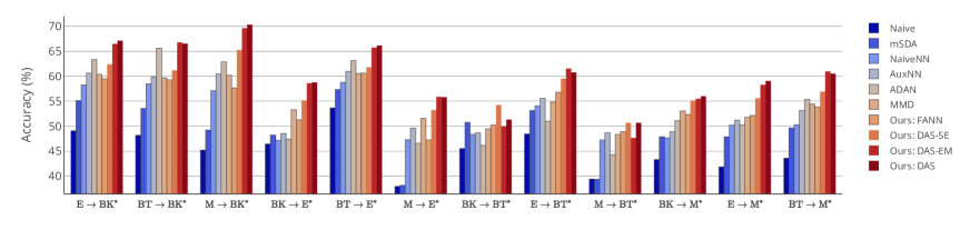
(a) Accuracy on the small-scale dataset under setting 1.

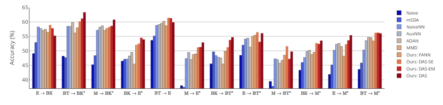
(b) Accuracy on the small-scale dataset under setting 2.

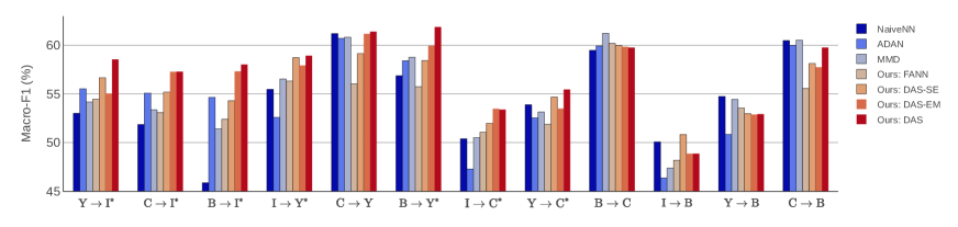
(c) Macro-F1 on the large-scale dataset.

Figure 1: Performance comparison. Average results over 5 runs with random initializations are reported for each neural method. ^∗ indicates that the proposed method (either of DAS, DAS-EM, DAS-SE) is significantly better than other baselines (baseline 1-6) with $p<0.05$ based on one-tailed unpaired t-test.

4.4 Training Details and Hyper-parameters

We initialize word embeddings using the 300-dimension GloVe vectors supplied by Pennington et al., (2014), which were trained on 840 billion tokens from the Common Crawl. For each pair of domains, the vocabulary consists of the top 10000 most frequent words. For words in the vocabulary but not present in the pre-trained embeddings, we randomly initialize them.

We set hyper-parameters of the CNN encoder following previous works Kim (2014); Yu and Jiang (2016) without specific tuning on our datasets. The window size is set to 3 and the size of the hidden layer is set to 300. The nonlinear activation function is Relu. For regularization, we also follow their settings and employ dropout with probability set to 0.5 on $\bm{\xi}_{i}$ before feeding it to the output layer $\mathcal{F}$, and constrain the $l_{2}$-norm of the weight vector $\theta_{f}$, setting its max norm to 3.

On the small-scale datasets and the Aamzon benchmark, $\lambda_{1}$ and $\lambda_{2}$ are set to 200 and 1, respectively, tuned on the development set of task E$\rightarrow$BK under setting 1. On the large-scale datasets, $\lambda_{1}$ and $\lambda_{2}$ are set to 500 and 0.2, respectively, tuned on I$\rightarrow$Y. We use a Gaussian curve $w(t)=\exp[-5(1-\frac{t}{t_{max}})^{2}]\lambda_{3}$ to ramp up the weight of the bootstrapping loss $\Omega$ from $0$ to $\lambda_{3}$, where $t_{max}$ denotes the maximum number of training epochs. We train 30 epochs for all experiments. We set $\lambda_{3}$ to 3 and $\alpha$ to 0.5 for all experiments.

The batch size is set to 50 on the small-scale datasets and the Amazon benchmark. We increase the batch size to 250 on the large-scale datasets to reduce the number of iterations. RMSProp optimizer with learning rate set to 0.0005 is used for all experiments.

4.5 Models for Comparison

We compare with the following baselines:

(1) Naive: A non-domain-adaptive baseline with bag-of-words representations and SVM classifier trained on the source domain.

(2) mSDA Chen et al. (2012): This is the state-of-the-art method based on discrete input features. Top 1000 bag-of-words features are kept as pivot features. We set the number of stacked layers to 3 and the corruption probability to 0.5.

(3) NaiveNN: This is a non-domain-adaptive CNN trained on source domain, which is a variant of our model by setting $\lambda_{1}$, $\lambda_{2}$, and $\lambda_{3}$ to zeros.

(4) AuxNN Yu and Jiang (2016): This is a neural model that exploits auxiliary tasks, which has achieved state-of-the-art results on cross-domain sentiment classification. The sentence encoder used in this model is the same as ours.

(5) ADAN Chen et al. (2017): This method exploits adversarial training to reduce representation difference between domains. The original paper uses a simple feedforward network as encoder. For fair comparison, we replace it with our CNN-based encoder. We train 5 iterations on the discriminator per iteration on the encoder and sentiment classifier as suggested in their paper.

(6) MMD: MMD has been widely used for minimizing domain discrepancy on images. In those works Tzeng et al. (2014); Long et al. (2017), variants of deep CNNs are used for encoding images and the MMDs of multiple layers are jointly minimized. In NLP, adding more layers of CNNs may not be very helpful and thus those models from image-related tasks can not be directly applied to our problem. To compare with MMD-based method, we train a model that jointly minimize the classification loss $L$ on the source domain and MMD between $\{\bm{\xi_{i}^{(s)}}|_{i=1}^{n_{s}}\}$ and $\{\bm{\xi_{i}^{(t)}}|_{i=1}^{n_{t}}\}$. For computing MMD, we use a Gaussian RBF which is a common choice for characteristic kernel.

In addition to the above baselines, we also show results of different variants of our model. DAS as shown in Algorithm 1 denotes our full model. DAS-EM denotes the model with only entropy minimization for semi-supervised learning (set $\lambda_{3}=0$). DAS-SE denotes the model with only self-ensemble bootstrapping for semi-supervised learning (set $\lambda_{2}=0$). FANN (feature-adaptation neural network) denotes the model without semi-supervised learning performed (set both $\lambda_{2}$ and $\lambda_{3}$ to zeros).

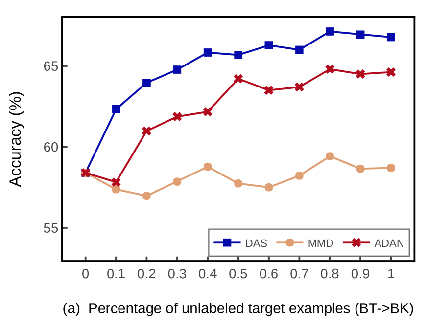
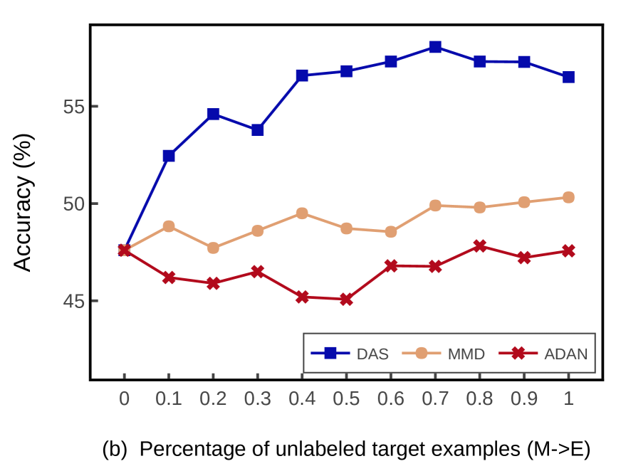
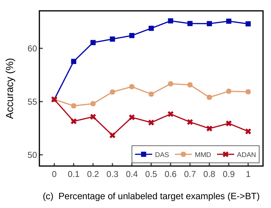
Figure 2: Accuracy vs. percentage of unlabeled target training examples.

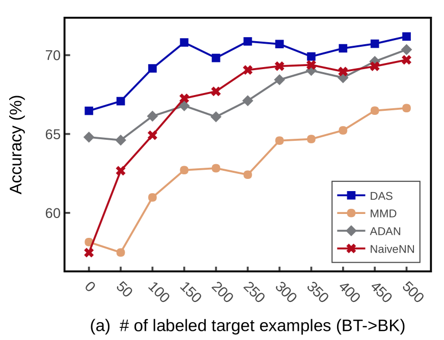
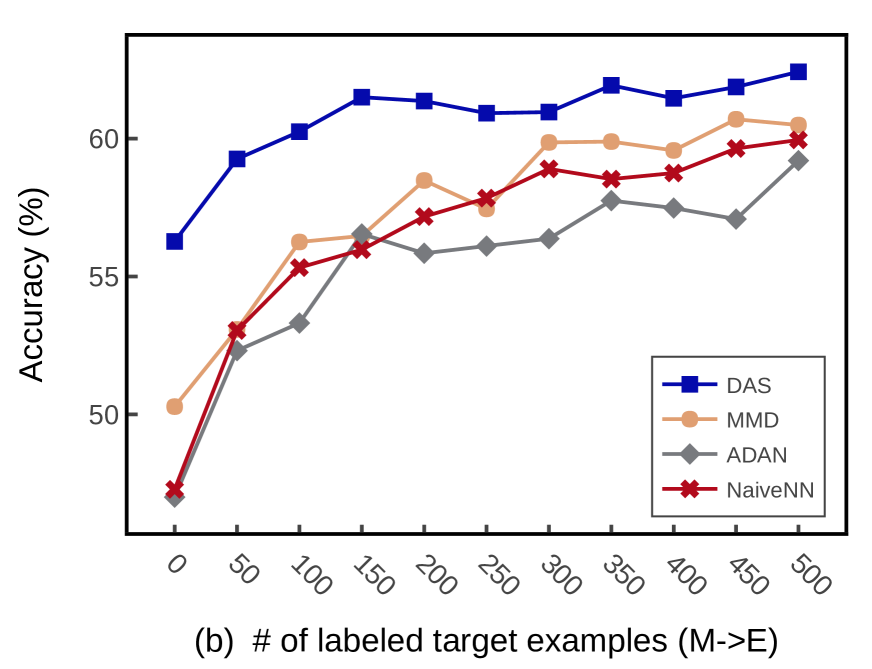
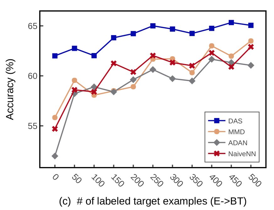
Figure 3: Accuracy vs. number of labeled target training examples.

4.6 Main Results

Figure 1 shows the comparison of adaptation results (see Appendix B for the exact numerical numbers). We report classification accuracy on the small-scale dataset. For the large-scale dataset, macro-F1 is instead used since the label distribution in the test set is extremely unbalanced. Key observations are summarized as follows. (1) Both DAS-EM and DAS-SE perform better in most cases compared with ADAN, MDD, and FANN, in which only feature adaptation is performed. This demonstrates the effectiveness of the proposed domain adaptive semi-supervised learning framework. DAS-EM is more effective than DAS-SE in most cases, and the full model DAS with both techniques jointly employed overall has the best performance. (2) When comparing the two settings on the small-scale dataset, all domain-adaptive methods generally perform better under setting 1. In setting 1, the target examples are balanced in classes, which can provide more diverse opinion-related features. However, when considering unsupervised domain adaptation, we should not presume the label distribution of the unlabeled data. Thus, it is necessary to conduct experiments using datasets that reflect real-life sentiment distribution as what we did on setting2 and the large-scale dataset. Unfortunately, this is ignored by most of previous works. (3) Word-embeddings are very helpful, as we can see even NaiveNN can substantially outperform mSDA on most tasks.

To see the effect of semi-supervised learning alone, we also conduct experiments by setting $\lambda_{1}=0$ to eliminate the effect of feature adaptation. Both entropy minimization and bootstrapping perform very badly in this setting. Entropy minimization gives almost random predictions with accuracy below 0.4, and the results of bootstrapping are also much lower compared to NaiveNN. This suggests that the feature adaptation component is essential. Without it, the learned target representations are less meaningful and discriminative. Applying semi-supervised learning in this case is likely to worsen the results.

best-value-at	highly-recommend-!	nars-are-amazing	beauty-store-suggested	since-i-love
good-value-at	highly-advise-!	ulta-are-fantastic	durable-machine-and	years-i-love
perfect-product-for	gogeous-absolutely-perfect	length-are-so	perfect-length-and	bonus-i-love
great-product-at	love-love-love	expected-in-perfect	great-store-on	appearance-i-love
amazing-product-$*$	highly-recommend-for	setting-works-perfect	beauty-store-for	relaxing-i-love

(a) NaiveNN

prices-my-favorite	so-nicely-!	purchase-thanks-!	feel-wonderfully-clean	are-really-cleaning
brands-my-favorite	more-affordable-price	buy-again-!	on-nicely-builds	washing-and-cleaning
very-great-stores	shampoo-a-perfect	without-hesitation-!	polish-easy-and	really-good-shampoo
great-bottle-also	an-excellent-value	buy-this-!	felt-cleanser-than	deeply-cleans-my
scent-pleasantly-floral	really-enjoy-it	discount-too-!	honestly-perfect-it	totally-moisturize-our

(b) FANN

bath-’s-wonderful	love-fruity-sweet	feeling-smooth-radiant	cleans-thoroughly-*	excellent-everyday-lotion
all-pretty-affordable	absorb-really-nicely	love-lavender-scented	loving-this-soap	affordable-cleans-nicely
it-delivers-fabulous	shower-lather-wonderfully	am-very-grateful	bed-of-love	fantastic-base-coat
and-blends-nicely	*-smells-fantastic	love-fruity-fragrances	shower-!-*	nice-gentle-scrub
heats-quickly-love	and-clean-excellent	perfect-beautiful-shimmer	radiant-daily-moisturizer	surprisingly-safe-on

(c) DAS

Table 2: Comparison of the top trigrams (each column) from the target domain (beauty) captured by the 5 most positive-sentiment-related CNN filters learned on E$\rightarrow$BT. $*$ denotes a padding.

4.7 Further Analysis

In Figure 2, we show the change of accuracy with respect to the percentage of unlabeled data used for training on three particular problems under setting 1. The value at $x=0$ denotes the accuracies of NaiveNN which does not utilize any target data. For DAS, we observe a nonlinear increasing trend where the accuracy quickly improves at the beginning, and then gradually stabilizes. For other methods, this trend is less obvious, and adding more unlabeled data sometimes even worsen the results. This finding again suggests that the proposed approach can better exploit the information from unlabeled data.

We also conduct experiments under a setting with a small number of labeled target examples available. Figure 3 shows the change of accuracy with respect to the number of labeled target examples added for training. We can observe that DAS is still more effective under this setting, while the performance differences to other methods gradually decrease with the increasing number of labeled target examples.

4.8 CNN Filter Analysis

In this subsection, we aim to better understand DAS by analyzing sentiment-related CNN filters. To do that, 1) we first select a list of the most related CNN filters for predicting each sentiment label (positive, negative neutral). Those filters can be identified according to the learned weights $\theta_{f}$ of the output layer $\mathcal{F}$. Higher weight indicates stronger relatedness. 2) Recall that in our implementation, each CNN filter has a window size of 3 with Relu activation. We can thus represent each selected filter as a ranked list of trigrams with highest activation values.

We analyze the CNN filters learned by NaiveNN, FANN and DAS respectively on task E$\rightarrow$BT under setting 1. We focus on E$\rightarrow$BT for study because electronics and beauty are very different domains and each of them has a diverse set of domain-specific sentiment expressions. For each method, we identify the top 10 most related filters for each sentiment label, and extract the top trigrams of each selected filter on both source and target domains. Since labeled source examples are used for training, we find the filters learned by the three methods capture similar expressions on the source domain, containing both domain-invariant and domain-specific trigrams. On the target domain, DAS captures more target-specific expressions compared to the other two methods. Due to space limitation, we only present a small subset of positive-sentiment-related filters in Table 2. The complete results are provided in Appendix C. From Table 2, we can observe that the filters learned by NaiveNN are almost unable to capture target-specific sentiment expressions, while FANN is able to capture limited target-specific words such as “clean” and “scent”. The filters learned by DAS are more domain-adaptive, capturing diverse sentiment expressions in the target domain.

5 Conclusion

In this work, we propose DAS, a novel framework that jointly performs feature adaptation and semi-supervised learning. We have demonstrated through multiple experiments that DAS can better leverage unlabeled data, and achieve substantial improvements over baseline methods. We have also shown that feature adaptation is an essential component, without which, semi-supervised learning is not able to function properly. The proposed framework could be potentially adapted to other domain adaptation tasks, which is the focus of our future studies.

Appendix A Results on Amazon Benchmark

Most previous works Blitzer et al. (2007); Pan et al. (2010); Glorot et al. (2011); Chen et al. (2012); Zhou et al. (2016) carried out experiments on the Amazon benchmark released by Blitzer et al. (2007). The dataset contains 4 different domains: Book (B), DVDs (D), Electronics (E), and Kitchen (K). Following their experimental settings, we consider the binary classification task to predict whether a review is positive or negative on the target domain. Each domain consists of 1000 positive and 1000 negative reviews respectively. We also allow 4000 unlabeled reviews to be used for both the source and the target domains, of which the positive and negative reviews are balanced as well, following the settings in previous works. We construct 12 cross-domain sentiment classification tasks and split the labeled data in each domain into a training set of 1600 reviews and a test set of 400 reviews. The classifier is trained on the training set of the source domain and is evaluated on the test set of the target domain. The comparison results are shown in Table 3.

S	T	Naive	mSDA	NaiveNN	AuxNN	ADAN	MMD	FANN	DAS-EM	DAS-SE	DAS
D	B	75.20	78.50	81.10	80.80	81.70	81.05	80.30	82.00∗	82.10∗	82.05∗
E	B	68.85	76.15	77.95	78.00	78.55	78.65	77.25	80.25∗	77.75	80.00∗
K	B	70.00	75.65	77.75	77.85	79.25	79.70	79.20	79.95	79.60	80.05∗
B	D	77.15	80.60	80.80	81.75	82.30	82.00	81.65	82.65	82.35	82.75∗
E	D	69.50	76.30	77.00	80.65	79.70	80.10	79.55	81.40∗	79.75	80.15
K	D	71.40	76.05	79.35	78.90	80.45	79.35	76.90	81.65∗	82.15∗	81.40∗
B	E	72.15	75.55	76.20	76.40	77.60	76.45	76.75	80.25∗	75.80	81.15∗
D	E	71.65	76.00	76.60	77.55	79.70	80.20	79.25	81.40∗	80.05	81.55∗
K	E	79.75	84.20	84.85	84.05	86.85	85.75	85.60	85.70	85.95	85.80
B	K	73.50	75.95	77.40	78.10	76.10	75.20	77.55	81.55∗	79.45∗	82.25∗
D	K	72.00	76.30	78.55	80.05	77.35	79.70	78.00	80.80	79.50	81.50∗
E	K	82.80	84.45	84.95	84.15	83.95	81.75	83.85	84.50	83.80	84.85
Average		73.66	77.98	79.38	79.85	80.29	80.00	79.65	81.84	80.68	81.96

Table 3: Accuracies on the Amazon benchmark. Average results over 5 runs with random initializations are reported for each neural method. ^∗ indicates that the proposed method (DAS-EM, DAS-SE, DAS) is significantly better than other baselines with $p<0.05$ based on one-tailed unpaired t-test.

Appendix B Numerical Results of Figure 1

Due to space limitation, we only show results in figures in the paper. All numerical numbers used for plotting Figure 1 are presented in Table 4. We can observe that DAS-EM, DAS-SE, and DAS all achieve substantial improvements over baseline methods under different settings.

S	T	Naive	mSDA	NaiveNN	AuxNN	ADAN	MMD	FANN	DAS-EM	DAS-SE	DAS
E	BK	49.07	55.13	58.26	60.62	63.32	60.38	59.59	66.48∗	62.37	67.12∗
BT	BK	48.17	53.53	58.48	59.86	65.62	59.66	59.28	66.78∗	61.17	66.53
M	BK	45.20	49.22	57.10	60.43	62.87	60.20	57.65	69.63∗	65.24∗	70.31∗
BK	E	46.43	48.22	47.15	48.45	47.42	53.32	51.27	58.59∗	55.15∗	58.73∗
BT	E	53.63	57.32	58.77	60.98	63.13	60.53	60.62	65.71∗	61.78	66.14∗
M	E	37.93	38.13	47.28	49.60	46.57	51.55	47.23	55.88∗	53.22∗	55.78∗
BK	BT	45.57	50.77	48.35	48.67	46.14	49.48	50.24	49.49	54.23∗	51.30∗
E	BT	48.43	53.13	54.07	55.58	50.98	54.83	56.78	61.53∗	59.52∗	60.76∗
M	BT	39.42	39.37	47.23	48.65	44.26	48.35	48.89	47.65	50.67∗	50.66∗
BK	M	43.32	47.88	47.67	48.87	51.10	53.04	52.35	55.47∗	55.13∗	55.98∗
E	M	41.83	47.88	50.21	51.19	50.23	51.81	52.14	58.28∗	55.60∗	59.06∗
BT	M	43.55	49.62	50.27	53.11	55.35	54.43	53.84	60.95∗	56.90∗	60.5∗
Average		45.21	49.18	52.07	53.84	53.92	54.80	54.15	59.74	57.58	60.24

(a) Accuracy on the small-scale dataset under setting 1

S	T	Naive	mSDA	NaiveNN	AuxNN	ADAN	MMD	FANN	DAS-EM	DAS-SE	DAS
E	BK	49.07	52.88	58.26	57.72	57.07	57.43	56.43	57.78	58.93	55.20
BT	BK	48.17	47.65	58.48	58.46	59.78	56.17	57.98	61.17∗	60.17∗	63.32∗
M	BK	45.20	48.33	57.10	58.15	58.67	57.08	57.75	58.62	58.25	60.77∗
BK	E	46.43	47.07	47.15	48.22	49.48	45.42	51.95	54.51∗	52.47∗	53.92∗
BT	E	53.63	55.12	58.77	59.08	59.45	60.24	58.67	61.27	61.42	59.83
M	E	37.93	37.40	47.28	49.43	47.00	48.72	48.92	51.28∗	51.18∗	52.88∗
BK	BT	45.57	49.63	48.35	47.80	47.52	45.43	49.83	53.72∗	51.23∗	54.67∗
E	BT	48.43	51.98	54.07	54.37	51.28	54.92	55.42	53.10	56.43∗	56.05∗
M	BT	39.43	37.73	47.23	46.92	45.73	46.68	48.48	47.18	51.57∗	49.73∗
BK	M	43.32	45.97	47.67	48.79	50.20	48.76	49.47	52.37∗	52.68∗	53.52∗
E	M	41.83	45.12	50.21	52.31	52.57	51.50	48.18	53.63∗	52.25	55.38∗
BT	M	43.55	45.78	50.27	53.55	54.68	54.55	53.41	56.24∗	56.23∗	56.02∗
Average		45.21	47.06	52.07	52.98	52.79	52.23	53.04	55.07	55.23	55.94

(b) Accuracy on the small-scale dataset under setting 2

S	T	NaiveNN	ADAN	MMD	FANN	DAS-EM	DAS-SE	DAS
Y	I	53.01	55.52	54.16	54.46	55.04	56.66∗	58.54∗
C	I	51.84	55.07	53.35	53.07	57.27∗	55.18	57.28∗
B	I	45.85	54.64	51.40	52.39	57.31∗	54.30	58.02∗
I	Y	55.46	52.57	56.52	56.30	57.92∗	58.72∗	58.92∗
C	Y	61.22	60.70	60.81	56.02	61.17	59.14	61.39
B	Y	56.86	58.42	58.77	55.72	59.94∗	58.43	61.87∗
I	C	50.38	47.27	50.49	51.04	53.46∗	51.97∗	53.38∗
Y	C	53.87	52.53	53.12	51.86	53.48	54.67∗	55.44∗
B	C	59.48	59.91	61.23	60.19	59.84	59.98	59.76
I	B	50.05	46.34	47.35	48.17	48.84	50.81	48.84
Y	B	54.73	50.82	54.43	53.54	52.87	52.95	52.91
C	B	60.47	59.99	60.52	55.56	57.74	58.12	59.75
Average		54.43	54.48	55.18	54.02	56.24	55.91	57.18

(c) Macro-F1 scores on the large-scale dataset

Table 4: Performance comparison. Average results over 5 runs with random initializations are reported for each neural method. ^∗ indicates that the proposed method (DAS, DAS-EM, DAS-SE) is significantly better than other baselines with $p<0.05$ based on one-tailed unpaired t-test.

Appendix C CNN Filter Analysis Full Results

As mentioned in Section 4.8, we conduct CNN filter analysis on NaiveNN, FANN, and DAS. For each method, we identify the top 10 most related filters for positive, negative, neutral sentiment labels respectively, and then represent each selected filter as a ranked list of trigrams with the highest activation values on it. Table 5, 6, 7 in the following pages illustrate the trigrams from the target domain (beauty) captured by the selected filters learned on E$\rightarrow$BT for each method.

We can observe that compared to NaiveNN and FANN, DAS is able to capture a more diverse set of relevant sentiment expressions on the target domain for each sentiment label. This observation is consistent with our motivation. Since NaiveNN, FANN and other baseline methods solely train the sentiment classifier on the source domain, the learned encoder is not able to produce discriminative features on the target domain. DAS addresses this problem by refining the classifier on the target domain with semi-supervised learning, and the overall objective forces the encoder to learn feature representations that are not only domain-invariant but also discriminative on both domains.

1	2	3	4	5
best-value-at	highly-recommend-!	nars-are-amazing	beauty-store-suggested	since-i-love
good-value-at	highly-advise-!	ulta-are-fantastic	durable-machine-and	years-i-love
perfect-product-for	gogeous-absolutely-perfect	length-are-so	perfect-length-and	bonus-i-love
great-product-at	love-love-love	expected-in-perfect	great-store-on	appearance-i-love
amazing-product-$*$	highly-recommend-for	setting-works-perfect	beauty-store-for	relaxing-i-love
6	7	8	9	10
store-and-am	office-setting-thanks	car-washes-!	speed-is-perfect	!-i-recommend
cleanser-and-am	locks-shimmering-color	price-in-stores	buttons-are-perfect	!-i-highly
olay-and-am	dirty-blonde-color	products-are-priced	unit-is-superb	shower-i-slather
daily-and-need	victoria-secrets-gorgeous	car-and-burning	spray-is-perfect	spots-i-needed
shower-and-noticed	dirty-pinkish-color	from-our-store	coverage-is-excellent	best-i-use

(a) NaiveNN

1	2	3	4	5
prices-my-favorite	so-nicely-!	purchase-thanks-!	feel-wonderfully-clean	are-really-cleaning
brands-my-favorite	more-affordable-price	buy-again-!	on-nicely-builds	washing-and-cleaning
very-great-stores	shampoo-a-perfect	without-hesitation-!	polish-easy-and	really-good-shampoo
great-bottle-also	an-excellent-value	buy-this-!	felt-cleanser-than	deeply-cleans-my
scent-pleasantly-floral	really-enjoy-it	discount-too-!	honestly-perfect-it	totally-moisturize-our
6	7	8	9	10
shower-or-cleaning	definitely-purchase-again	more-affordable-price	absolutely-wonderful-!	felt-cleaner-than
water-onto-my	definitely-buy-again	a-perfect-length	perfect-for-running	flat-iron-through
bleach-your-towels	perfect-for-my	an-exceptional-value	concealer-for-my	rubbed-grease-on
pump-onto-my	definitely-order-again	’ve-enjoyed-it	moisturizing-for-my	deeply-cleans-my
water-great-for	super-happy-to	pretty-decent-layer	super-glue-even	being-cleaner-after

(b) FANN

1	2	3	4	5
bath-’s-wonderful	love-fruity-sweet	feeling-smooth-radiant	cleans-thoroughly-*	excellent-everyday-lotion
all-pretty-affordable	absorb-really-nicely	love-lavender-scented	loving-this-soap	affordable-cleans-nicely
it-delivers-fabulous	shower-lather-wonderfully	am-very-grateful	bed-of-love	fantastic-base-coat
and-blends-nicely	*-smells-fantastic	love-fruity-fragrances	shower-!-*	nice-gentle-scrub
heats-quickly-love	and-clean-excellent	perfect-beautiful-shimmer	radiant-daily-moisturizer	surprisingly-safe-on
6	7	8	9	10
shower-lather-wonderfully	highly-recommend-!	excellent-fragrance-and	its-unique-smoothing	forgeous-gragrance-mist
affordable-cleans-nicely	definitely-recommend-!	fantastic-for-daytime	smooth-luxurious-texture	wonderful-bedtime-scent
peels-great-price	love-love-!	wonderfully-moisturizing-and	’s-extremely-gentle	love-essie-polish
daughter-loves-this	highly-advise-!	lathers-great-cleans	’s-affordable-combination	perfect-beautiful-shimmer
cleans-great-smells	time-advise-!	delightful-shampoo-works	absorbs-quite-well	fantastic-coverage-hydrates

(c) DAS

Table 5: Top 5 trigrams from the target domain (beauty) captured by the top 10 most positive-sentiment-related CNN filters learned on E$\rightarrow$BT. $*$ denotes a padding.

1	2	3	4	5
pads-ruined-my	simply-threw-out	hours-after-trying	junk-drawer-$*$	contacted-manufacturer-about
highly-disappointed-and	reviewer-pointed-out	minutes-after-rinsing	refund-time-!	minutes-not-worth
dryers-blew-my	extracts-broke-into	disappointed-after-trying	total-fake-wen	’ve-owned-this
completely-worthless-didn’t	actually-threw-out	lips-after-trying	waste-your-time	hour-unless-it
am-disappointed-and	clips-barely-keep	dry-after-shampooing	total-fail-!	results-they-claim
6	7	8	9	10
were-awful-garbage	two-failed-attempts	auto-ship-sent	refund-and-dispose	broke-don’t-fix
what-awful-garbage	a-mistake-save	am-returning-to	refund-spend-your	sent-me-expired
and-utter-waste	a-definite-return	am-unable-to	wouldn’t-recommend-!	wearing-false-eyelashes
are-absolute-garbage	a-pathetic-limp	am-pale-ghost	not-buy-dunhill	a-temporary-fix
piece-of-junk	a-total-disappointment	got-returned-and	not-worth-returning	a-disappointment-cheap

(a) NaiveNN

1	2	3	4	5
nasty-sunburn-lol	the-worse-mascaras	stale-very-unhappy	actually-hurts-your	a-return-label
bother-returning-them	it-caused-patchy	were-horrible-failures	didn’t-bother-returning	stay-away-completely
fails-miserably-at	lifeless-disaster-enter	send-this-crap	it-hurts-your	like-bug-quit
minutes-auric-needs	it-fails-miserably	were-awful-garbage	didn’t-exist-in	a-defective-brown
severely-burned-me	feel-worse-leaving	were-horribly-red	skin-horribly-after	’d-refund-the
6	7	8	9	10
worse-with-exercise	not-stink-your	it-fails-miserably	got-progressively-worse	stopped-working-for
worse-and-after	mistake-save-your	is-ineffective-apart	gave-opposite-result	uncomfortable-i-returned
unable-to-return	nothing-!-by	but-horribly-unhealthy	another-epic-fail	i-am-returning
worse-my-face	nothing-happened-!	a-pathetic-limp	got-horribly-painful	stopped-working-shortly
poorly-in-step	nothing-save-your	a-worse-job	was-downright-painful	not-waterproof-makeup

(b) FANN

1	2	3	4	5
poorly-designed-product	a-refund-spend	completely-waste-of	smells-disgusting-!	burning-rubber-stench
defective-dryer-promising	a-refund-save	of-junk-*	smells-horribly-like	began-smelling-vomit
disgusting-smelling-thing	i-regret-spending	were-awful-garbage	does-not-straighten	reaction-and-wasted
hurts-your-scalp	just-wouldn’t-spend	worthless-waste-of	’s-false-advertising	control-and-smelled
hurts-your-hair	looked-washed-out	throwing-money-away	a-disgusting-cheap	using-this-disgusting
6	7	8	9	10
super-irritating-!	got-promptly-broke	sore-and-painful	it-caused-patchy	painful-it-hurt
strong-reaction-and	after-ive-washed	is-simply-irritating	layer-hydrogenated-alcohols	unnecessary-health-risks
really-burned-and	after-several-attempts	tight-and-uncomfortable	the-harmful-uva	uncomfortable-to-wear
very-pasty-and	this-stuff-stinks	drying-and-irritating	my-severe-dark	stinging-your-eyes
super-streaky-and	again-i-threw	goopy-and-unpleasant	a-allergic-reaction	unbearable-to-wear

(c) DAS

Table 6: Top 5 trigrams from the target domain (beauty) captured by the top 10 most negative-sentiment-related CNN filters learned on E$\rightarrow$BT. $*$ denotes a padding.

1	2	3	4	5
purpose-cologne-splash	okay-cord-was	hands-feet-elbows	aggressive-in-general	but-its-okay
other-hanae-mori	cocamide-dea-is	been-sealed-tight	pimples-in-general	it-moisturizes-okay
the-mavala-peeled	coily-conditioner-is	stainless-steel-blackhead	biotin-in-general	but-moisturizes-keeps
avoid-hair-pulling	flaky-dandruff-is	severely-tight-chest	dimethicone-is-terrible	but-don’t-expect
cause-rashes-stinging	quickly-cord-is	thick-nasty-callouses	but-in-general	it-lathers-ok
6	7	8	9	10
pretty-damaged-from	darker-olive-complexion	doesn’t-mind-pushing	producto-por-los	feeling-didn’t-last
daughter-suffers-from	stronger-healthier-or	kinda-doesn’t-its	unstuck-frownies-$*$	curls-didn’t-last
teenager-suffers-from	natural-ingredient-however	kinda-kinky-coily	they-push-$*$	extra-uv-protection
tissue-damage-during	vitamin-enriched-color	okay-job-of	uva-rays-uva	garnier-fructis-curl
the-damage-on	natural-ingredients-$*$	intended-purpose-that	tend-to-slip	the-mavala-after

(a) NaiveNN

1	2	3	4	5
worse-and-after	maybe-a-refund	very-disappointing-waste	my-ears-are	pretty-neutral-neither
worse-before-improving	ok-mask-i	ok-but-clean	my-neck-line	ok-so-if
unable-to-return	ok-pining-it	ok-but-will	cause-unsightly-beads	ok-during-pregnancy
unless-your-entire	ok-try-i	ok-but-didn’t	my-sporadic-line	kinda-annoying-if
horrible-in-execution	ok-tho-i	ok-nothing-special	your-ear-is	ok-this-seems
6	7	8	9	10
uncomfortable-i-returned	sticky-lathers-and	some-fading-when	are-very-painful	its-also-convenient
weak-they-bend	quickly-deep-cleans	real-disappointment-the	are-less-painful	that-also-my
claimed-faulty-$*$	but-elegant-bottle	especially-noticeable-after	are-a-pain	that-may-make
suffers-from-wind	beat-the-price	progressively-worse-during	about-sum-damage	that-allows-your
as-defective-$*$	and-reasonably-priced	style-unfortunately-the	offered-no-pain	its-helpful-to

(b) FANN

1	2	3	4	5
’m-kinda-pale	darker-but-nope	ok-but-horrible	noticeable-i-avoid	same-result-mediocre
a-terrible-headache	gray-didn’t-cover	ok-but-didn’t	however-i-lean	it-caused-patchy
but-kinda-annoying	makeup-doesn’t-sweat	okay-but-doesn’t	but-otherwise-ok	doesn’t-cause-flare
’m-kinda-mad	dark-spots-around	okay-however-it	but-im-deciding	the-harmful-uva
i-kinda-stopped	moist-but-thats	unfortunately-straight	however-i-prefer	rather-unpleasant-smell
6	7	8	9	10
kinda-annoying-if	brutal-winter-however	higher-rating-because	nothing-for-odor	but-darker-*
pretty-bad-breakage	summer-color-however	slight-burnt-rubber	kinda-recommend-this	slightly-darker-shade
my-slight-discoloration	beige-shade-however	noticeable-tan-since	not-recommend-if	somewhat-pale-affect
smells-kinda-bad	is-okay-however	somewhat-pale-affect	noticeable-but-non	but-somewhat-heavy
look-kinda-crappy	bit-greasy-however	kinda-pale-so	nothing-special-moderate	bit-dull-heavy

(c) DAS

Table 7: Top 5 trigrams from the target domain (beauty) captured by the top 10 most neutral-sentiment-related CNN filters learned on E$\rightarrow$BT. $*$ denotes a padding.

References

- Blitzer et al. (2007) John Blitzer, Mark Dredze, and Fernando Pereira. 2007. Biographies, Bollywood, boom-boxes and blenders: domain adaptation for sentiment classification. In Annual Meeting of the Association for Computational Linguistics.
- Chen et al. (2012) Minmin Chen, Zhixiang Xu, Kilian Q. Weinberger, and Fei Sha. 2012. Marginalized denoising autoencoders for domain adaptation. In The 29th International Conference on Machine Learning.
- Chen et al. (2017) Xilun Chen, Yu Sun, Ben Athiwarakun, Claire Cardie, and Kilian Weinberger. 2017. Adversarial deep averaging networks for cross-lingual sentiment classifier. In Arxiv e-prints arXiv:1606.01614.
- Dai et al. (2007) Wenyuan Dai, Gui rong Xue, Qiang Yang, and Yong Yu. 2007. Transferring naive Bayes classifiers for text classification. In AAAI Conference on Artificial Intelligence.
- Ganin and Lempitsky (2015) Yaroslav Ganin and Victor Lempitsky. 2015. Unsupervised domain adaptation by backpropagation. In International Conference on Machine Learning.
- Glorot et al. (2011) Xavier Glorot, Antoine Bordes, and Yoshua Bengio. 2011. Domain adaptation for large-scale sentiment classification: a deep learning approach. In The 28th International Conference on Machine Learning.
- Grandvalet and Bengio (2004) Yves Grandvalet and Yoshua Bengio. 2004. Semi-supervised learning by entropy minimization. In Neural Information Processing Systems.
- Gretton et al. (2012) Arthur Gretton, Karsten M. Borgwardt, Malte J. Rasch, Bernhard Schölkopf, and Alexander Smola. 2012. A kernel two-sample test. Journal of Machine Learning Research, 13:723–773.
- He and McAuley (2016) Ruining He and Julian McAuley. 2016. Ups and downs: modeling the visual evolution of fashion trends with one-class collaborative filtering. In WWW.
- He et al. (2011) Yulan He, Chenghua Lin, and Harith Alani. 2011. Automatically extracting polarity-bearing topics for cross-domain sentiment classification. In ACL.
- Jiang and Zhai (2007) Jing Jiang and ChengXiang Zhai. 2007. Instance weighting for domain adaptation in NLP. In Annual Meeting of the Association for Computational Linguistics.
- Kim (2014) Yoon Kim. 2014. Convolutional neural networks for sentence classification. In Conference on Empirical Methods in Natural Language Processing.
- Laine and Aila (2017) Samuli Laine and Timo Aila. 2017. Temporal ensembling for semi-supervised learning. In International Conference on Learning Representation.
- Li et al. (2017) Zheng Li, Yun Zhang, Ying Wei, Yuxiang Wu, and Qiang Yang. 2017. End-to-end adversarial memory network for cross-domain sentiment classification. In The 26th International Joint Conference on Artificial Intelligence.
- Long et al. (2015) Mingsheng Long, Yue Cao, Jianmin Wang, and Michael I. Jordan. 2015. Learning transferable features with deep adaptation networks. In International Conference on Machine Learning.
- Long et al. (2017) Mingsheng Long, Han Zhu, Jianmin Wang, and Michael I. Jordan. 2017. Deep transfer learning with joint adaptation networks. In International Conference on Machine Learning.
- McAuley et al. (2015) Julian J. McAuley, Christopher Targett, Qinfeng Shi, and Anton van den Hengel. 2015. Image-based recommendations on styles and substitutes. In The 38th International ACM SIGIR Conference on Research and Development in Information Retrieval.
- Mikolov et al. (2013) Tomas Mikolov, Ilya Sutskever, Kai Chen, Greg Corrado, and Jeffrey Dean. 2013. Distributed representations of words and phrases and their compositionality. In Neural Information Processing Systems.
- Pan et al. (2010) Sinno Jialin Pan, Xiaochuan Ni, Jian-Tao Sun, Qiang Yang, and Zheng Chen. 2010. Cross-domain sentiment classification via spectral feature alignment. In The 19th International World Wide Web Conference.
- Pennington et al. (2014) Jeffrey Pennington, Richard Socher, and Christopher D Manning. 2014. GloVe: Global vectors for word representation. In Conference on Empirical Methods in Natural Language Processing.
- Tang et al. (2015) Duyu Tang, Bing Qin, and Ting Liu. 2015. Learning semantic representation of users and products for document level sentiment classification. In Annual Meeting of the Association for Computational Linguistics.
- Tzeng et al. (2014) Eric Tzeng, Judy Hoffman, Ning Zhang, Kate Saenko, and Trevor Darrell. 2014. Deep domain confusion: maximizing for domain invariance. In Arxiv e-prints arXiv:1412.3474.
- Wu et al. (2009) Dan Wu, Wee Sun Lee, Nan Ye, and Hai Leong Chieu. 2009. Domain adaptive bootstrapping for named entity recognition. In Conference on Empirical Methods in Natural Language Processing.
- Wu and Huang (2016) Fangzhao Wu and Yongfeng Huang. 2016. Sentiment domain adaptation with multiple sources. In Annual Meeting of the Association for Computational Linguistics.
- Yang et al. (2017) Wei Yang, Wei Lu, and Vincent W. Zheng. 2017. A simple regularization-based algorithm for learning cross-domain word embeddings. In Conference on Empirical Methods in Natural Language Processing.
- Yang and Eisenstein (2014) Yi Yang and Jacob Eisenstein. 2014. Fast easy unsupervised domain adaptation with marginalized structured dropout. In Annual Meeting of the Association for Computational Linguistics.
- Yu and Jiang (2016) Jianfei Yu and Jing Jiang. 2016. Learning sentence embeddings with auxiliary tasks for cross-domain sentiment classification. In Conference on Empirical Methods in Natural Language Processing.
- Zhou et al. (2015) Guangyou Zhou, Tingting He, Wensheng Wu, and Xiaohua Tony Hu. 2015. Linking heterogeneous input features with pivots for domain adaptation. In The 24th International Joint Conference on Artificial Intelligence.
- Zhou et al. (2016) Guangyou Zhou, Zhiwen Xie, Jimmy Xiangji Huang, and Tingting He. 2016. Bi-transferring deep neural networks for domain adaptation. In Annual Meeting of the Association for Computational Linguistics.
- Zhuang et al. (2015) Fuzhen Zhuang, Xiaohu Cheng, Ping Luo, Sinno Jialin Pan, and Qing He. 2015. Supervised representation learning: transfer learning with deep autoencoders. In The 24th International Joint Conference on Artificial Intelligence.