ELUCID. VI: Cosmic variance of galaxy distribution in the local Universe

Abstract

Halo merger trees are constructed from ELUCID, a constrained $N$-body simulation in the Sloan Digital Sky Survey (SDSS) volume. These merger trees are used to populate dark matter halos with galaxies according to an empirical model of galaxy formation. Mock catalogs in the SDSS sky coverage are constructed, which can be used to study the spatial distribution of galaxies in the low-$z$ Universe. These mock catalogs are used to quantify the cosmic variance in the galaxy stellar mass function (GSMF) measured from the SDSS survey. The GSMF estimated from the SDSS magnitude-limited sample can be affected significantly by the presence of the under-dense region at $z<0.03$, so that the low-mass end of the function can be underestimated significantly. Several existing methods designed to deal with the effects of the cosmic variance in the estimate of GSMF are tested, and none is found to be able to fully account for the cosmic variance. We propose a method based on the conditional stellar mass functions in dark matter halos, which can provide an unbiased estimate of the global GSMF. The application of the method to the SDSS data shows that the GSMF has a significant upturn at $M_{*}<10^{9.5}\,h^{-1}{\rm M_{\odot}}$, which has been missed in many earlier measurements of the local GSMF.

1. Introduction

The Universe contains prominent structures up to $\sim 100\,{\rm Mpc}$, only reaching homogeneity on much large scales (e.g. Peebles, 1980; Davis et al., 1985). The properties of galaxies and other objects, which form and evolve in the cosmic web, are expected to be affected by their large-scale environments. Thus, astronomical observations, which are always made in limited volumes in the Universe, can be affected by the cosmic variance (CV) caused by spatial variations of the statistical properties of cosmic objects, such as galaxies, due to the presence of large scale structure. Because of CV, statistics obtained from a sample that covers a specific volume in the Universe may be different from those expected for the Universe as a whole. Erroneous inferences would then be made if such biased observational data were used to constrain models.

Cosmic variance (CV) is a well known problem (e.g. Somerville et al., 2004; Jha et al., 2007; Driver & Robotham, 2010; Moster et al., 2011; Marra et al., 2013; Keenan et al., 2013; Wojtak et al., 2014; Whitbourn & Shanks, 2014, 2016), and various attempts have been made to deal with it. One way is to analyze different (sub-)samples, e.g. obtained from the Jackknife sampling of the observational data, and to use the variations among them to have some handle on the CV. However, this can only provide information about the variance within the total sample itself, but not that of the total sample relative to a fair sample of the Universe. Another way is to use the spatial distribution of bright galaxies (a density-defining population), which can be observed in a large volume, to quantify the CV expected in sub-volumes (e.g. Driver & Robotham, 2010), or to re-scale (or correct) the number density of faint galaxies observed in a smaller volume, as was done by Baldry et al. (2012) in their estimate of galaxy stellar mass functions in the GAMA sample. However, this method relies on the assumption that galaxies of different luminosities/masses have similar spatial distributions, which may not be true. The same problem also exists in the maximal likelihood method (e.g. G. Efstathiou, 1988), where galaxy luminosity function is explicitly assumed to be independent of environment. Yet another way is to estimate the CV expected from a given sample using simple, analytic models for the clustering properties of galaxies on large scales. Along this line, Somerville et al. (2004) tested the effects of the CV on different scales, and proposed the use of either the two-point correlation function of galaxies, or the combination of the linear density field with halo bias models (e.g. Mo & White, 1996; Sheth et al., 2001), to predict the CV of different surveys. Similarly, Moster et al. (2011) carried out an investigation of the CV expected in observations of the galaxy populations at different redshifts, using the linear density field predicted by the ${\rm\Lambda CDM}$ model combined with a bias model that takes into account the dependence of galaxy distribution on galaxy mass and redshift. Unfortunately, such an approach does not take into account observational selection effects. More importantly, this approach only gives a statistical estimate of the CV but does not measure the deviation of a specific sample from a fair sample. Finally, one can also use a large number of mock galaxy samples, either obtained directly from hydrodynamic simulations, or from N-body simulation-based semi-analytic (SAM) and empirical models, to quantify how the sample-to-sample variation of the statistical measure in question depends on sample volume. However, this needs a large set of simulations for each model, analyzed in a way that takes into account the observational selection effects in the data, which in practice is costly and time consuming. Furthermore, the same as the approach based on galaxy clustering statistics, this approach can only provide a statistical statement of the expected CV, but does not provide a way to correct the variance of a specific sample.

Can one develop a systematic method to study the cosmic variance, and to quantify and correct biases that are present in observational data? The answer is yes, and the key is to use constrained simulations. Indeed, if one can accurately reconstruct the initial conditions for the formation of the structures in which the observed galaxy population reside, one can then carry out simulations with such initial conditions in a sufficiently large box that contains the constrained volume, so that the large box can be used as a fair sample, while the constrained region can be used to model the observational data. By comparing the statistics obtained from the mock samples with those obtained from the whole box, one can quantify and correct the CV in the observational data.

In the past few years, the ELUCID collaboration has embarked on the development of a method to accurately reconstruct the initial conditions responsible for the density field in the low-$z$ Universe (Wang et al., 2014). As demonstrated by various tests (Wang et al., 2014; Wang et al., 2016), the reconstruction method is much more accurate than other methods that have been developed, and works reliably even in highly non-linear regimes. The initial conditions in a $500\,h^{-1}{\rm{Mpc}}$ box that contains the main part of the SDSS volume have already been obtained, and a high resolution $N$-body simulation, run with $(3072)^{3}$ particles, has been carried out with these initial conditions in the current $\Lambda$CDM cosmology (Wang et al., 2016).

In the present paper, we use the dark matter halo merger trees constructed from the ELUCID simulation to populate simulated halos with model galaxies predicted by the empirical galaxy formation model developed by Lu et al. (2014a, 2015b, thereafter L14, L15). The model galaxies in the constrained volume are then used to construct mock catalogs that contain the same CV as the real SDSS sample. We compare galaxy stellar mass functions (GSMF) estimated from the mock catalogs with that obtained from the total simulation box to quantify the CV within the SDSS volume. Finally, we propose a method based on the conditional stellar mass or luminosity distribution in dark matter halos to correct for the CV in the observed GSMF. As we will see, the CV can be very severe in the low-mass end of the GSMF obtained from methods commonly adopted, and the low-mass end slope of the true GSMF in the low-$z$ Universe may be significantly steeper than those published in the literature.

The structure of the paper is as follows. In §2 we describe methods to implement Monte Carlo halo merger trees in simulated merger trees, so as to extend all trees down to a mass resolution sufficient for our purpose. In §3 we populate simulated halos with galaxies using an empirical model of galaxy formation, and construct a number of mock catalogs to mimics the SDSS survey both in spatial distribution and physical properties. In §4 we examine in detail the cosmic variance in the estimates of the GSMF, and show how commonly adopted methods to measure the galaxy luminosity function (GLF) and GSMF fail to account for the CV. We also propose and test a new method to correct for CV in GLF and GSMF, and apply it to the real SDSS data to obtain the CV-corrected GLF and GSMF. Finally, a brief summary of our main results is presented in §5.

Throughout the paper, we define the GSMF as $\Phi(M_{*})=\mathrm{d}N/\mathrm{d}V/\mathrm{d}\log M_{*}$, which is the number of galaxies per unit volume per unit stellar mass in logarithmic space, and define the GLF in $\rm X$-band as $\Phi(M_{\rm X})={\rm d}N/{\rm d}V/{\rm d}(M_{\rm X}-5\log h)$, which is the number of galaxies per unit volume per unit magnitude. The magnitude $M_{\rm X}$ is $k$-corrected to redshift $0.1$ without evolution correction, unless specified otherwise.

2. Merger trees of dark matter halos from the ELUCID simulation

2.1. The simulation

We use the ELUCID simulation carried out by Wang et al. (2016) to model the dark matter halo population, their formation histories, and spatial distribution. This is an $N$-body simulation that uses L-GADGET, a memory optimized version of GADGET-2 (Springel, 2005), to follow the evolution of $3072^{3}$ dark matter particles (each with a mass of $3.088\times 10^{8}\,h^{-1}{\rm M_{\odot}}$) in a periodic cubic box with side length of $500\,h^{-1}{\rm{Mpc}}$ in co-moving units. The cosmology used is the one based on WMAP5 (Dunkley et al., 2009; Komatsu et al., 2009): a flat Universe with $\Omega_{K}=0$; a matter density parameter $\Omega_{\rm m,0}=0.258$; a cosmological constant $\Omega_{\Lambda,0}=0.742$; a baryon density parameter $\Omega_{\rm B,0}=0.044$; a Hubble constant $H_{0}=100h\ \mathrm{km\ s^{-1}\ \,{\rm Mpc}^{-1}}$ with $h=0.72$; and a Gaussian initial density field with power spectrum $P(k)\propto k^{n}$, with $n=0.96$ and with the amplitude specified by $\sigma_{8}=0.80$. The simulation is run from redshift $z=100$ to $z=0$, with outputs recorded at 100 snapshots between $z=18.4$ and $z=0.0$.

The initial conditions (phases of Fourier modes) of the density field are those obtained from the reconstruction based on the halo-domain method of Wang et al. (2009) and the Hamiltonian Markov Chain Monte Carlo (HMC) method (Wang et al., 2013, 2014), constrained by the distributions of dark matter halos represented by galaxy groups and clusters selected from the SDSS redshift survey (Yang et al., 2007; Yang et al., 2012). As shown in Wang et al. (2016) with the use of mock catalogs, more than $95\%$ of the groups with masses above $10^{14}\,h^{-1}{\rm M_{\odot}}$ can be matched with the simulated halos of similar masses, with a distance error tolerance of $\sim 4\,h^{-1}{\rm{Mpc}}$, and massive structures such as the Coma cluster and the Sloan Great Wall can be well reproduced in the reconstruction. Thus, the use of the constrained simulation from ELUCID allows us not only to model accurately the large-scale environments within which observed galaxies reside, but also to recover, at least partially, the formation histories of the massive structures seen in the local Universe.

2.2. The construction of halo merger trees

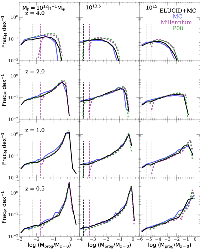
Figure 1.— Conditional progenitor mass functions (mean fraction of mass in progenitors in per unit progenitor mass $M_{\rm prog}/M_{z=0}$ bin in logarithmic space) of dark matter halos from different kinds of merging trees, for different $z=0$ halos of different masses (each column) and for progenitors at different redshifts (each row). Black solid: halo merger trees obtained from ELUCID simulation repaired by Monte-Carlo-based trees. Blue solid: P08 (Parkinson et al., 2008) Monte Carlo trees generated with the WMAP5 cosmology. Purple dashed: Millennium (Springel, 2005) FOF halo merger trees. Green dashed: P08 Monte Carlo trees with Millennium cosmology. The two vertical solid lines show the 20 particles mass resolution of halos in ELUCID and Millennium simulations, respectively.

Halos and their sub-halos with more than 20 particles are identified with the friend-of-friend (FOF) and SUBFIND algorithms (Springel et al., 2005). To be safe, we only use halos identified in the simulation with masses $M_{\rm h}\geq M_{\rm th}=10^{10}\,h^{-1}{\rm M_{\odot}}$. However, this mass resolution is not sufficient to resolve lower mass halos in which star formation may still be significant, particularly at high $z$. In order to trace the star formation histories in halos to high redshifts, we need to reach a halo mass of about $10^{9}\,h^{-1}{\rm M_{\odot}}$, below which star formation is expected to be unimportant due to photo-ionization heating (e.g. Babul & Rees, 1992; Thoul & Weinberg, 1996). Here we adopt a Monte Carlo method to extend the merger trees of the simulated halos down to a mass limit, $10^{9}\,h^{-1}{\rm M_{\odot}}$. Jiang & van den Bosch (2014) have tested the performances of several different methods of generating Monte Carlo halo merger trees, and found that the method of Parkinson et al. (2008, thereafter P08) consistently provides the best match to the halo merging trees obtained from $N$-body simulations. We therefore adopt the P08 method.

We join the P08 Monte Carlo trees to the halo merger trees obtained from the simulation through the following steps:

1. For each simulated halo merger tree $T$, we eliminate halos that have masses below $M_{\rm th}=10^{10}\,h^{-1}{\rm M_{\odot}}$ but have no progenitors more massive than $M_{\rm th}$. The purpose of the second condition is to preserve halos which once had masses larger than $M_{\rm th}$ but have become less massive later due to stripping and/or mass loss.

2. For each halo $H$ that is not eliminated in $T$, we generate a Monte Carlo tree $t$ (down to $10^{9}\,h^{-1}{\rm M_{\odot}}$), rooted from a halo $h$ that has the same mass and the same redshift as $H$, and eliminate all halos more massive than $10^{10}\,h^{-1}{\rm M_{\odot}}$ in $t$.

3. We add $t$ to $H$. The procedure is repeated for all halos with masses above $10^{10}\,h^{-1}{\rm M_{\odot}}$ in all trees in the ELUCID simulation, so that all such halos have merger trees extended to $10^{9}\,h^{-1}{\rm M_{\odot}}$.

4. For halos with masses below $10^{10}\,h^{-1}{\rm M_{\odot}}$ at $z=0$, their merger trees are entirely generated with the Monte Carlo method. Note that these halos are not identified from the simulation, but can be used to model galaxies in such low-mass halos when needed.

With these steps, we obtain ‘repaired’ halo merger trees that have a mass resolution of $10^{9}\,h^{-1}{\rm M_{\odot}}$, with halos more massive than $10^{10}\,h^{-1}{\rm M_{\odot}}$ sampled entirely by the simulation, and the less massive ones modeled by Monte-Carlo trees. Fig. 1 shows the conditional progenitor mass functions of dark matter halos, defined as the fraction of mass in progenitors per logarithmic mass, for merger trees rooted from different masses, and for progenitors at different redshifts. Our results, obtained by combining the simulated trees above the mass resolution $M_{\rm th}$ with the Monte Carlo merging trees generated with the P08 model below the mass limit, are shown by the black solid lines, and compared with the merger trees generated entirely with the P08 model. Overall, the progenitor mass distributions we obtain match well those obtained from the Monte Carlo method, indicating that our merger trees are reliable.

Since galaxies form and evolve in dark matter halos, our ‘repaired’ halo merger trees from the ELUCID simulation provide the basis to link galaxy properties to dark matter halos, and can be used in combinations with halo-based methods of galaxy formation, such as abundance matching, semi-analytic and other empirical models, to populate halos with galaxies. The method can, in principle, be applied to simulated halos with any mass resolution and with any cosmology, to extend halo merger trees to a sufficiently low mass, as long as reliable Monte Carlo trees can be generated. We note that our merger trees do not include high order sub-halos, i.e. sub-halos in sub-halos. In the next section, we apply the empirical model, developed in L14 and L15, to follow galaxy formation and evolution in dark matter halos, based on our repaired halo merger trees.

3. Populating halos with galaxies

In this section, we describe the L14, L15 empirical method, developed by Lu et al. (2014a, 2015b), to populate galaxies in the halo merger trees described in the previous section. Briefly, we assign a central galaxy to each distinctive halo and give it an appropriate star formation rate (SFR) according to the empirical model. We then evolve all galaxies in the current snapshot to the next, following the accretion of galaxies by dark matter halos and the mergers of galaxies. The stellar masses for both central and satellite galaxies are obtained by integrating the stellar contents along their histories. Finally, observable quantities, such as luminosity and apparent magnitude, are obtained from a stellar population synthesis model.

3.1. The empirical model of galaxy formation

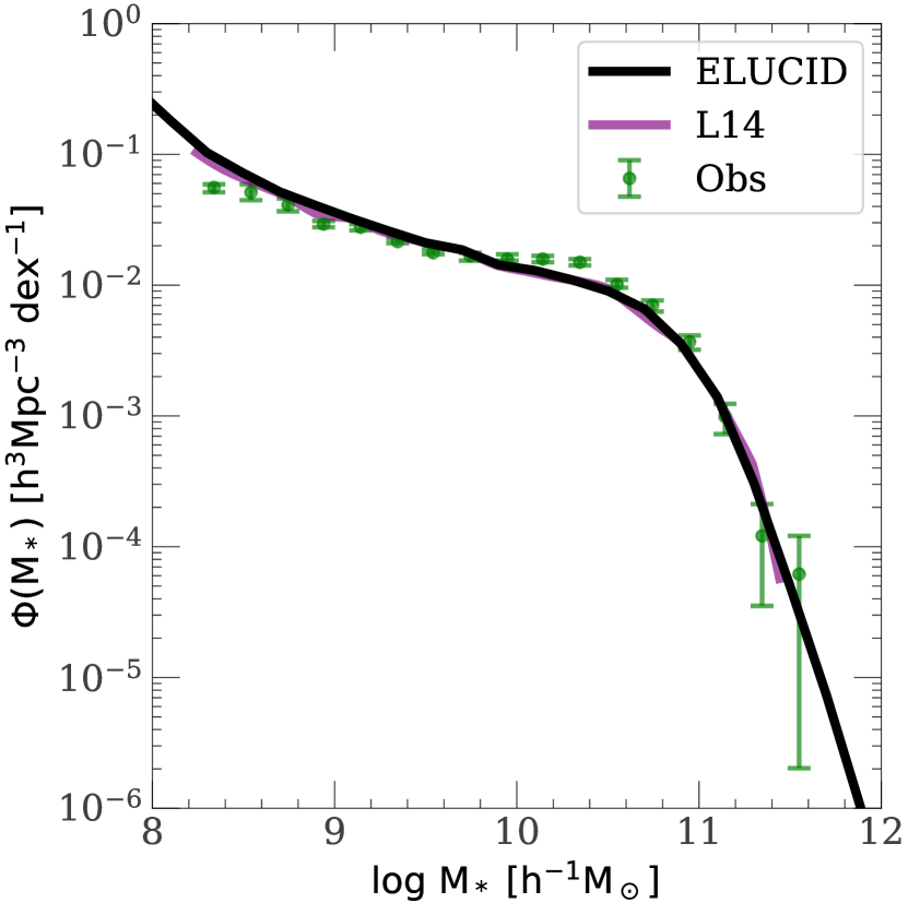
Figure 2.— Galaxy stellar mass functions at redshift $z=0$. Black solid line: model galaxies based on our repaired trees. Purple solid line: from  Lu et al., 2014a, based on Monte Carlo halo merger trees. Green dots with error bars: from observational result which is used by L14 to calibrate the model.

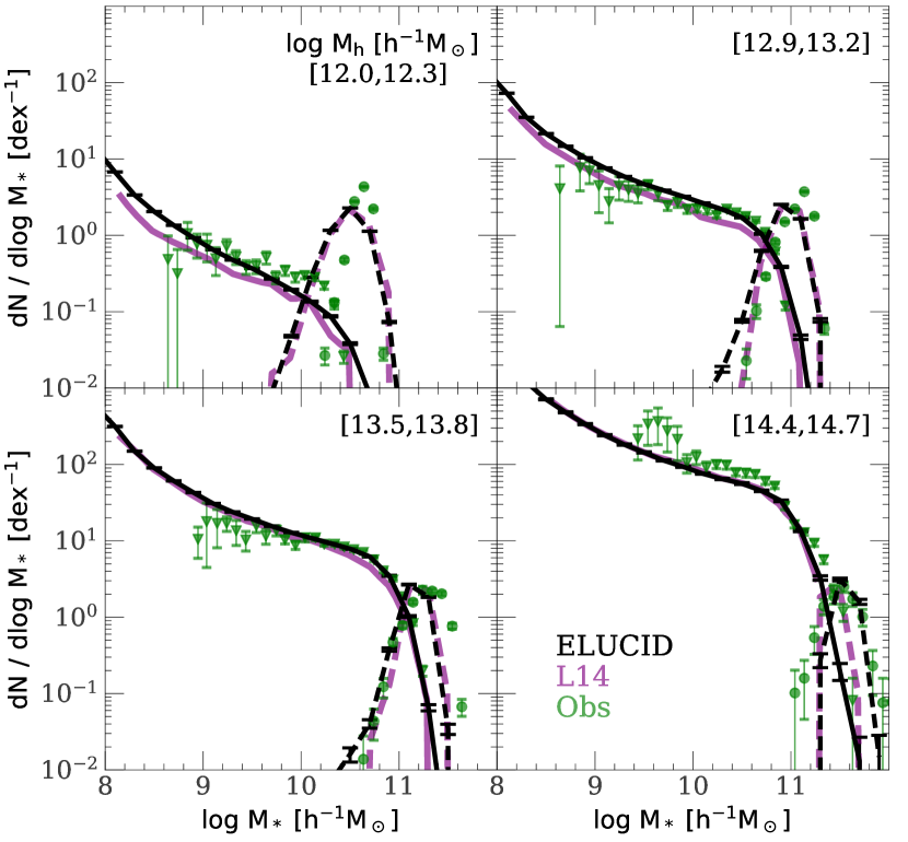
Figure 3.— Conditional stellar mass functions in halos with different mass $M_{\rm h}$ (as indicated in each panel) at redshift $z=0$. Black lines: model galaxies based on our repaired trees, for central galaxies (dashed) and satellite galaxies (solid). The error bars indicate the standard deviations among 100 bootstrap resamplings. Purple lines: from Lu et al., 2014a, based on Monte Carlo halo merger trees, for central galaxies (dashed) and satellite galaxies (solid). Green markers with error bars: from observational result of Yang et al., 2008, for central galaxies (circles) and satellite galaxies (triangles).

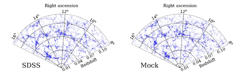
Figure 4.— Spatial distribution of SDSS (left panel) and mock (right panel) galaxies. Selections are made for all galaxies with $r\leq 17.6$ in the redshift range $[0.01,\ 0.12]$ in the Sloan NGC region. Only galaxies in a $4^{\circ}$ declination slice are plotted.

In the model of L14 and L15, SFR of a central galaxy is assumed to depend on the halo mass $M_{\rm halo}$ and redshift $z$ as

$$\begin{split}{\rm SFR}&(M_{\rm halo},z)=\\ &\varepsilon\frac{f_{\rm B}M_{\rm halo}}{\tau_{0}}(1+z)^{\kappa}(1+X)^{\alpha}\left(\frac{X+R}{X+1}\right)^{\beta}\left(\frac{X}{X+R}\right)^{\gamma}\end{split}$$ (1)

where $\tau_{0}=1/(10H_{0})$, $\kappa=3/2$. $f_{\rm B}=\Omega_{\rm B,0}/\Omega_{\rm m,0}$ is the cosmic baryon fraction, and $\varepsilon$ and $\beta$ are time-independent model parameters. The parameters, $\alpha$ and $\gamma$, are assumed to be time-dependent, given by

$$\alpha=\alpha_{0}(1+z)^{\alpha^{{}^{\prime}}}$$ (2)

and

$$\gamma=\left\{\begin{aligned} &\gamma_{a}&\mathrm{if}\ z<z_{c}\\ &(\gamma_{a}-\gamma_{b})(\frac{z+1}{z_{c}+1})^{\gamma^{{}^{\prime}}}+\gamma_{b}&\mathrm{if}\ z\geq z_{c}\end{aligned}\right.$$ (3)

where $\alpha_{0}$, $\alpha^{{}^{\prime}}$, $\gamma_{a}$, $\gamma_{b}$ and $z_{c}$ are time-independent model parameters. In L14 and L15, both $\alpha$ and $\gamma$ are chosen to be time-dependent to make the model compatible with the observed galaxy stellar mass functions (GSMFs) at different redshifts and the composite conditional luminosity function of cluster galaxies at redshift $z=0$ (see also Lim et al., 2017b). All the model parameters are determined by fitting the model predictions to a set of observational data (see the original papers for details). Here we adopt the parameters listed in L14 (denoted by ’Model III SMF+CGLF’ in this paper), which are based on a cosmology consistent with the WMAP5 cosmology (Dunkley et al., 2009; Komatsu et al., 2009) used here.

Once a dark matter halo hosting a galaxy is accreted by a bigger halo, the central galaxy in it is assumed to become a satellite galaxy, and thus experience satellite-specific processes, such as tidal stripping and ram-pressure stripping, which may reduce and quench its star formation. L14 modelled the SFR in satellites as

$${\rm SFR}(M_{*},z)={\rm SFR}(t_{\rm accr})\exp\left[-\frac{t-t_{\rm accr}}{\tau(M_{*})}\right]$$ (4)

with

$$\tau(M_{*})=\tau_{*,0}\exp(-M_{*}/M_{*,c})\,.$$ (5)

Here $M_{*}$ is the current mass of the satellite galaxy, $\tau_{*,0}$ and $M_{*,c}$ are time-independent model parameters, and $t_{\rm accr}$ is the cosmic time at which the host halo of the galaxy is accreted. After accretion, the satellite halo and the galaxies it hosts are expected to experience dynamical friction, which causes them to move towards the inner part of the new host halo. The satellites may then merger with the central galaxy located near the center. We follow L14 and use an empirical model to determine the time when the merger occurs:

$$\Delta t=0.216\frac{Y^{1.3}}{\ln(1+Y)}\exp(1.9\eta)\frac{r_{\rm halo}}{v_{\rm halo}},$$ (6)

where $Y=M_{\rm cen}/M_{\rm sat}$ is the ratio of mass between the central halo and the satellite halo at the time when the accretion occurs, and $r_{\rm halo}$ and $v_{\rm halo}$ are the virial radius and virial velocity of the central halo (e.g. Boylan-Kolchin et al., 2008). The parameter, $\eta$, describes the specific orbital angular momentum, and is assumed to follow a probability distribution $P(\eta)=\eta^{1.2}(1-\eta)^{1.2}$ (e.g. Zentner et al., 2005). After merger, a fraction of $f_{\rm TS}$ of the stellar mass of the satellite is added to the central galaxy, with $f_{\rm TS}$ a model parameter.

The ingredients given above can be used to predict the stellar mass and SFR of both central and satellite galaxies. In order to make predictions for galaxy luminosities in different bands, we also need the metallicities of stars. We use the mean metallicity - stellar mass relation given by Gallazzi et al. (2005) to assign metallicities to galaxies according to their masses. A simple stellar population synthesis model, based on the Bruzual & Charlot (2003) with a Chabrier initial mass function (Chabrier, 2003), is adopted to obtained the mass to light ratio of formed star, and the mass loss due to stellar evolution.

We note that the L14 model, which is based on Monte-Carlo merger trees, does not take into account some special events that exist in numerical simulations. In simulated merger trees, some sub-halos were main halos at some early times, accreted into other systems as satellites later, and were eventually ejected and became main halos again. For such cases, we treat the galaxy in the sub-halo as a satellite galaxy even after the sub-halo is ejected. The ejected sub-halos are then treated as new main halos after ejection. This implementation does not make much physical sense, but best mimic the Monte Carlo merger trees in which sub-halos are never ejected, and all halos at a given time are treated equally without depending on whether or not they have gone through a big halo. Such an implementation is necessary, as the model parameters given by L14 are calibrated by using Monte-Carlo merger trees.

Fig. 2 shows the galaxy stellar mass function (GSMF) of model galaxies at redshift z = 0, in black solid line, in comparison with the result of L14 (purple solid line). As one can see, the L14 result is well reproduced over wide ranges of stellar masses, which demonstrates that our implementation of the L14 model with the ELUCID halo merger trees are reliable, as long as the general galaxy GSMF is concerned. For reference, we also include the observational data points (green dots with error bars) that were used in L14 to constrain their model parameters.

As a more demanding test, we compare in Fig. 3 the conditional galaxy stellar mass functions (CGSMFs) in halos of different masses at redshift $z=0$ obtained from the ELUCID halo merger trees with those given by L14. Here again we see a good agreement between the two. Since the CGSMF gives the average number of galaxies of a given stellar mass in a halo of a given mass, a good match in CGSMFs also implies that the spatial clustering of galaxies as a function of stellar mass is also reproduced.

3.2. Galaxy occupation in dark matter halos

To use our model galaxies to construct mock catalogs, we need to assign spatial positions and peculiar velocities to galaxies in each halo in the simulation according to the halo occupation distributions (HODs) obtained from the empirical model described above. Here we adopt a sub-halo abundance matching method that links galaxies in a halo to the sub-halos in it. As shown in Wang et al. (2016), the sub-halo population can be identified reliably from the ELUCID simulation for sub-halos with masses down to $\sim 10^{10}\,h^{-1}{\rm M_{\odot}}$. The abundance matching goes as follows. For a given halo, we first rank galaxies in descending order of stellar mass and sub-halos in descending order of halo mass. Here the mass of a sub-halo is that at the time when the sub-halo was first accreted into its host. Note that sub-halos both identified directly from the simulation and added using Monte Carlo merger trees (see §2.2) are used. For sub-halos identified in the simulation, their positions and velocities are those given by the SUNFIND. For the Monte Carlo sub-halos that are joined to the simulated halos, on the other hand, we assign random positions according to the NFW profile (Navarro et al., 1997) with concentration parameters given by Zhao et al. (2009), and their velocities are drawn from a Gaussian distribution with dispersion appropriate for the density profile assumed. For sub-halos that are rooted from a $z=0$ Monte Carlo halo, the galaxies hosted by them are usually too faint to be relevant; they are only included for completeness, but actually are not used in constructing the mock catalog. Finally, the position and velocity of the sub-halo are assigned to the galaxy that has the same rank. For those galaxies that do not have sub-halo counter-parts, their positions and velocities are assigned randomly according to the NFW profile. This method can be used to construct volume limited samples within the entire simulation box down to stellar masses $\sim 10^{8}\,h^{-1}{\rm M_{\odot}}$, with full phase space information obtained from the simulated sub-halos. This is sufficient for most of our purposes.

3.3. The SDSS mock catalog

With full information about the luminosities and phase space coordinates for individual galaxies, it is straightforward to make mock catalogs using galaxies in the constrained volume and applying the same selection criteria as in the observation. For each model galaxy in the simulation box, we assign to it a cosmological redsfhit, $z_{\rm cos}$, according to its distance to a virtual observer, and the observed redshift, $z_{\rm obs}$, is given by $z_{\rm cos}$ together with its line-of-sight (los) peculiar velocity, $v_{\rm los}$:

$$z_{\rm obs}=z_{\rm cos}+(1+z_{\rm cos})\frac{v_{\rm los}}{c}\,,$$ (7)

with $c$ the speed of light. Here the location of the virtual observer and the coordinate system are determined by the orientation of the SDSS volume in the simulation box. SDSS apparent magnitudes in $u$, $g$, $r$, $i$, and $z$ are assigned to each galaxy according to its luminosities in the corresponding bands. For our SDSS mock sample, we select all galaxies in the SDSS Northern-Galactic-Cap (NGC) region with redshifts $0.01<z<0.12$ and with magnitude $r\leq 17.6$.

Fig. 4 shows the real SDSS galaxies (left) and the mock galaxies (right) in the same slice in the SDSS sky coverage. It is clear that the distribution of the mock galaxies is very similar to that of the real galaxies. The large scale structures in the local Universe, such as the Sloan Great Wall at redshift $\approx 0.08$, are well reproduced. Thus, the mock catalog can be used to investigate both the properties of the galaxy population in the cosmic web, and the large scale clustering of galaxies. In particular, since all galaxies above our mass resolution limit, which is about $10^{8}\,h^{-1}{\rm M_{\odot}}$, are modeled in the entire simulation box, a comparison of the statistical properties between the SDSS mock catalog and the whole simulation box carries information about the CV of the SDSS sample.

4. Cosmic variance in galaxy stellar mass functions

The realistic model catalogs described above have many applications, such as to study the relationships between galaxies and the the mass density field, and to investigate the galaxy population in different components of the cosmic web. Here we use them to analyze and quantify the cosmic variances (CV) in the measurements of the galaxy stellar mass function (GSMF) and luminosity function (GLF). We first use model galaxies in the whole simulation box to quantify the CV as a function of sample volume and galaxy mass. We then use the SDSS mock catalog to examine the CV in the SDSS, and to investigate different estimates of the GSMF/GLF in their abilities to account for the CV. We propose and test a new method that can best correct for the CV. Finally, we apply our method to the SDSS catalog to obtain GLF and GSMF that are free of the CV.

4.1. Cosmic variance as a function of sample volume and galaxy mass

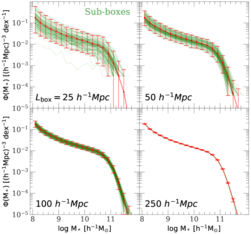
Figure 5.— GSMFs at $z=0$ in sub-boxes in the $500\,h^{-1}{\rm{Mpc}}$ box of ELUCID simulation. For each sub-box size $L_{\rm box}\leq 100h^{-1}{\rm Mpc}$, 100 sub-boxes without overlap are randomly chosen in the simulation box, while for $L_{\rm box}=250\,h^{-1}{\rm{Mpc}}$, all the 8 sub-boxes are used. The GSMFs of individual sub-boxes are shown by the green curves in each panel. The average over the sub-boxes of the same size is given by the red line in each panel. Error bars covering $96\%$ ($2\sigma$) range among different sub-boxes are also plotted.

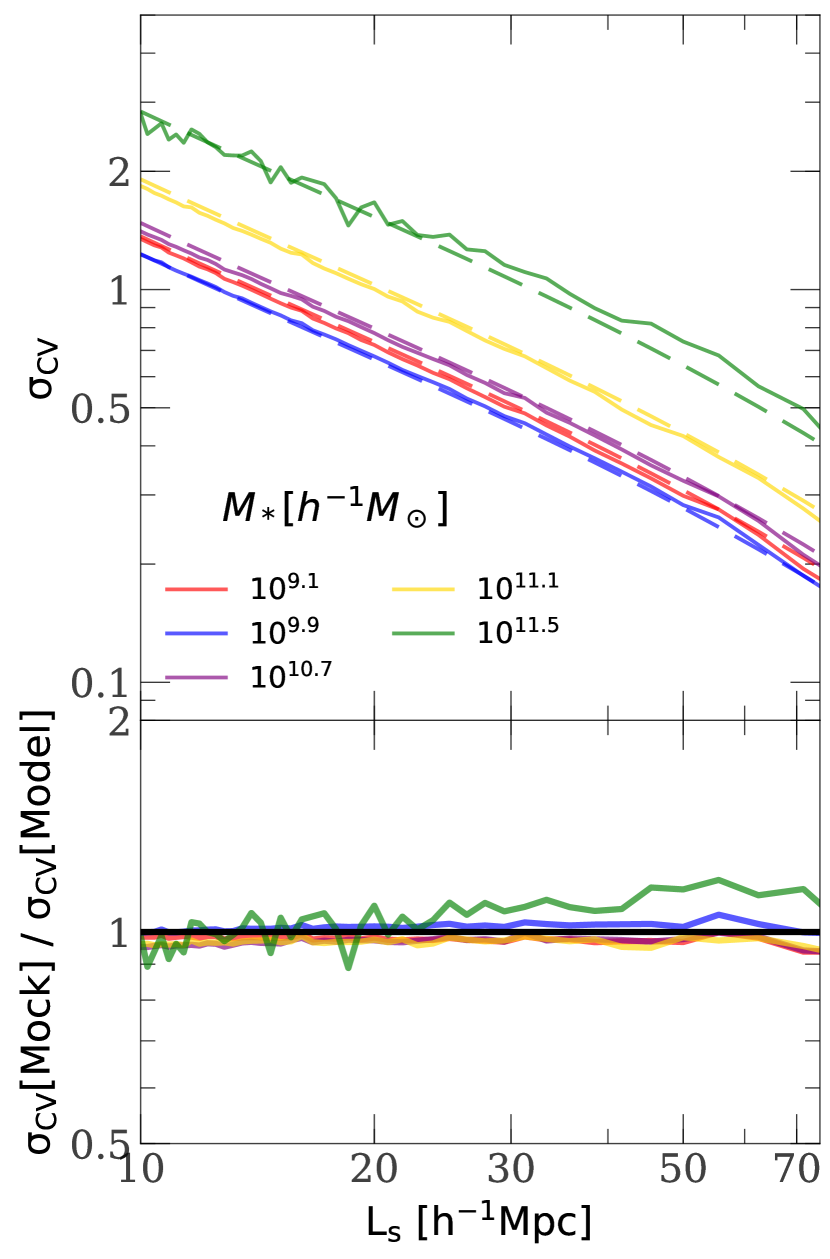
Figure 6.— Upper panel: Cosmic variance $\sigma_{\rm CV}$ as a function of the characteristic size of sample $L_{\rm s}$ and stellar mass $M_{*}$, as indicated in the panel. Solid lines are $\sigma_{\rm CV}$ estimated from the mock sample, while dashed lines are from the fitting formula. Lower panel: Ratio of $\sigma_{\rm CV}$ between the mock sample and model prediction. The black solid line indicates the ratio of $1.0$.

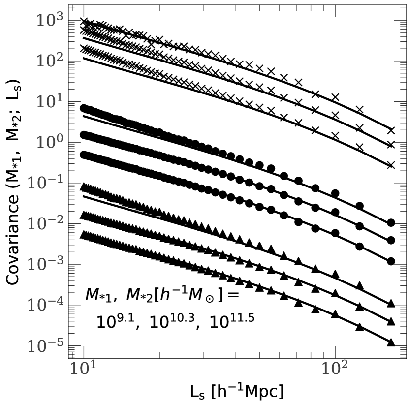
Figure 7.— The covariance, ${\rm Cov}(M_{*,1},\ M_{*,2};\ L_{\rm s})$, of the GSMF between two stellar masses, $M_{*,1}$ and $M_{*,2}$, as a function of the characteristic sample size $L_{s}$. Symbols show results obtained from the mock sample. Different $M_{*,1}$ are represented by different symbols: $M_{*,1}[\,h^{-1}{\rm M_{\odot}}]=10^{9.1},\ 10^{10.3},\ 10^{11.5}$, from bottom up, scaled by $0.01,\ 1,\ 100$, respectively, for clarity. Different $M_{*,2}$ with the same $M_{*,1}$ are re-scaled by $0.3,\ 1,\ 1.2$, for $M_{*,2}[\,h^{-1}{\rm M_{\odot}}]=10^{9.1},\ 10^{10.3},\ 10^{11.5}$, respectively. The solid curves are model predictions.

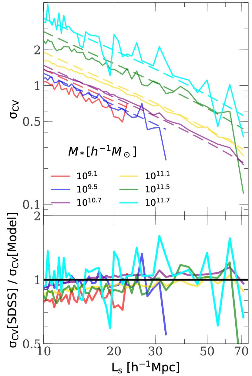
Figure 8.— The model of cosmic variance compared with SDSS data. Upper panel: Cosmic variance $\sigma_{\rm CV}$ of the GSMF as a function of the characteristic sample size $L_{\rm s}$, for galaxies of different stellar masses, $M_{*}$, as shown by different colors. Solid lines are $\sigma_{\rm CV}$ estimated from the SDSS sample, while dashed lines are predictions of the fitting model. Lower panel: The ratio of $\sigma_{\rm CV}$ between the SDSS sample and the model. The black horizontal line indicates the ratio of $1.0$.

To quantify the effects of CV, we partition the whole $500^{3}\ h^{-3}\mathrm{Mpc}^{3}$ simulation box into sub-boxes, each with a given size $L_{\rm s}$, without overlap. For each sub-box $i$ we calculate the galaxy number density $n_{g,i}(M_{*};L_{s})$. Fig. 5 shows the GSMFs obtained for 100 sub-boxes with sizes $L_{\rm s}=25$, $50$, $100$, and $250\,h^{-1}{\rm{Mpc}}$, respectively. The results of individual sub-boxes are shown by the green lines, while the average and the $2\sigma$ variance ($96\%$) among the GSMFs are shown by the red curve and bars, respectively. As expected, the scatter among the sub-boxes decreases as the sub-box size increases. For instance, the scatter for $L_{\rm s}=50\,h^{-1}{\rm{Mpc}}$ is about $\approx 0.3\ {\rm dex}$ over almost the entire stellar mass range, while it is smaller than $10\%$ for $L_{\rm s}=250\,h^{-1}{\rm{Mpc}}$.

Theoretically, the galaxy number density $n_{g}$ is related to the mass density $\rho_{m}$ by a stochastic bias relation:

$$\delta_{g}=b\delta_{m}+\epsilon\,,$$ (8)

where $\delta_{g}=(n_{g}/{\overline{n}}_{g})-1$ and $\delta_{m}=(\rho_{m}/{\overline{\rho}}_{m})-1$, with ${\overline{n}}_{g}$ and ${\overline{\rho}}_{m}$ being the mean number density of galaxies and the mean density of mass in the Universe. The coefficient, $b$, is the bias parameter, which characterizes the deterministic part of the bias relation, and $\epsilon$ is the stochastic part. If the galaxy number density field is a Poisson sampling of the mass density field, then the variance in the galaxy density can be written as

$$\sigma_{t}^{2}=\sigma^{2}_{\rm CV}+\sigma_{\rm P}^{2},$$ (9)

where $\sigma_{P}=N^{-1/2}$ is due to Poisson fluctuation. Assuming linear bias, the deterministic part, which we refer to as the cosmic variance (CV), can be written as:

$$\sigma_{\rm CV}^{2}(M_{*};L_{s})=b^{2}(M_{*})\sigma_{m}^{2}(L_{s}),$$ (10)

where $L_{s}$ is the characteristic size of the sample, and $\sigma_{m}(L_{s})$ is the rms of the mass fluctuation on the scale of $L_{s}$.

Motivated by this, we model $\sigma_{\rm CV}$ using the GSMF obtained from simulated galaxies. The number density $n_{g,i}$ of all sub-boxes are synthesized to give the mean value, ${\overline{n}}_{g}(M_{*};L_{s})$, and the variance, $\sigma_{t}^{2}(M_{*};\ L_{s})$. We use ${\overline{n}}_{g}$ to estimate the expected Poisson variance, $\sigma_{\rm P}^{2}$, and use equation (9) to estimate $\sigma_{\rm CV}^{2}(M_{*};L_{s})$ by subtracting the Poisson part from the total variance. Equation (10) is then used to fit the dependence of CV on stellar mass and the size of sub-box. We find that the $L_{s}$-dependence can be well described by

$$\log\sigma_{m}(x)=p_{0}+p_{1}x+p_{2}x^{2}+p_{3}x^{3}\,,$$ (11)

where $x=\log(L_{s}/\,h^{-1}{\rm{Mpc}})$, and $p_{0}=1.53$, $p_{1}=-2.02$, $p_{2}=0.92$, and $p_{3}=-0.25$, while the $M_{*}$ dependence by

$$\log b(y)=q_{0}+q_{1}y+q_{2}y^{2}+q_{3}y^{3}\,,$$ (12)

where $y=\log(M_{*}/\,h^{-1}{\rm M_{\odot}})$, and $q_{0}=-16.04$, $q_{1}=5.79$, $q_{2}=-0.68$, and $q_{3}=0.026$.

Fig. 6 shows the comparison between $\sigma_{\rm CV}$ obtained direct from the simulated galaxy sample and the model prediction as a function of $L_{s}$ for galaxies of different $M_{*}$, as represented by different lines. The fitting formulae work well over the range from $10^{8}\,h^{-1}{\rm M_{\odot}}$ to $10^{11.6}\,h^{-1}{\rm M_{\odot}}$ in $M_{*}$, and from $10\,h^{-1}{\rm{Mpc}}$ to $125\,h^{-1}{\rm{Mpc}}$ in $L_{s}$.

The above prescription also provides a model for the covariance matrix of the cosmic variance. Consider the covariance matrix, $C$, of the densities between galaxies of masses $M_{*,1}$ and $M_{*,2}$. The bias model described above gives

$$C(M_{*,1},M_{*,2};L_{s})=b(M_{*,1})b(M_{*,2})\sigma_{m}^{2}(L_{s}).$$ (13)

Fig. 7 shows the ratio between the measured $C$ and the model predictions as a function of $L_{s}$ for a number of $(M_{*,1},M_{*,2})$ pairs. Overall the model matches the measurements well. Some discrepancies can be seen for massive galaxies and small $L_{s}$, where the model prediction is slightly lower than that measured from the simulation data.

We can compare the CV model calibrated above with that obtained from SDSS data. To this end, we estimate the total variance, the Poisson variance, and the cosmic variance using sub-boxes of given $L_{s}$ that are fully contained by the SDSS volume, within which the sample is complete for a given $M_{*}$. In order to estimate the variance among sub-boxes reliably, we only present cases where at least 10 sub-boxes are available. The results, plotted in Fig. 8, show that the SDSS measurements follow the model predictions for $10<L_{s}<75\,h^{-1}{\rm{Mpc}}$ and $M_{*}>10^{9}\,h^{-1}{\rm M_{\odot}}$. Note that we did not fit the $\sigma_{\rm CV}$ for $M_{*}>10^{11.6}\,h^{-1}{\rm M_{\odot}}$, but the extrapolation seems to match the SDSS measurements well even for such stellar masses. For $M_{*}<10^{9}\,h^{-1}{\rm M_{\odot}}$, the variance obtained from the SDSS becomes significantly lower than the model prediction. As we will see below, this deviation is caused by the fact that the local volume, within which such galaxies can be observed, does not sample the galaxy population fairly.

To summarize, the simple model presented above provides a useful way to estimate the level of CV expected in the measurements of the GSMF. This variance, which is produced by the fluctuations of the cosmic density field, should be combined with the Poisson variance from number counting to estimate the total variance in the uncertainty in the GSMF. This is particularly the case where the galaxy population is observed in a small volume and the cosmic variance is large than the counting error. In real applications, other types of uncertainties, such as errors in photometry, redshift, and stellar mass estimate, should also be modeled properly along with the CV described here.

4.2. Cosmic variances in the SDSS volume

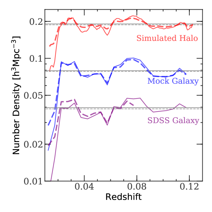
Figure 9.— Galaxy and halo number densities at different redshift $z$ in the Sloan sky coverage, from $z=0.01$ to $0.12$. Red lines are for simulated halos (Solid: halos with $M_{\rm h}>10^{12}\,h^{-1}{\rm M_{\odot}}$, offset by $\times 60.0$; Dashed: $10^{8}\leq M_{\rm h}\leq 10^{12}\,h^{-1}{\rm M_{\odot}}$). Blue lines are for mock galaxies based on the empirical model (Solid: $M_{*}>10^{10.5}\,h^{-1}{\rm M_{\odot}}$, offset by $\times 22.0$; Dashed: $10^{9.5}\leq M_{*}\leq 10^{10.5}\,h^{-1}{\rm M_{\odot}}$, offset by $\times 4.8$). Purple lines are for SDSS galaxies (Solid: galaxies with $M_{r}<-20.5$, offset by $\times 8.0$; Dashed: $-20.5\leq M_{r}\leq-19.5$, offset by $\times 4.4$). Horizontal lines are the mean number densities in the corresponding volumes.

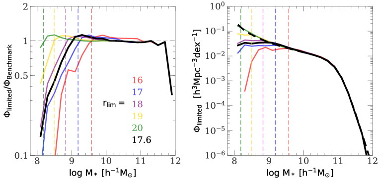
Figure 10.— The galaxy stellar mass functions (GSMF), $\Phi(M_{*})$, estimated using the V-max method from SDSS magnitude-limited mock samples with different magnitude limits, $r_{\rm lim}$, as shown in the left panel. Right panel shows the absolute values of the GSMF, with the benchmark shown by the black dashed line. The black solid shows the result for $r_{\rm lim}=17.6$, the magnitude limit of the SDSS survey. The left panel shows the ratio of GSMF between the magnitude-limited samples and benchmark. In each panel, the vertical dashed lines indicate the stellar masses corresponding to the break at $z=0.03$.

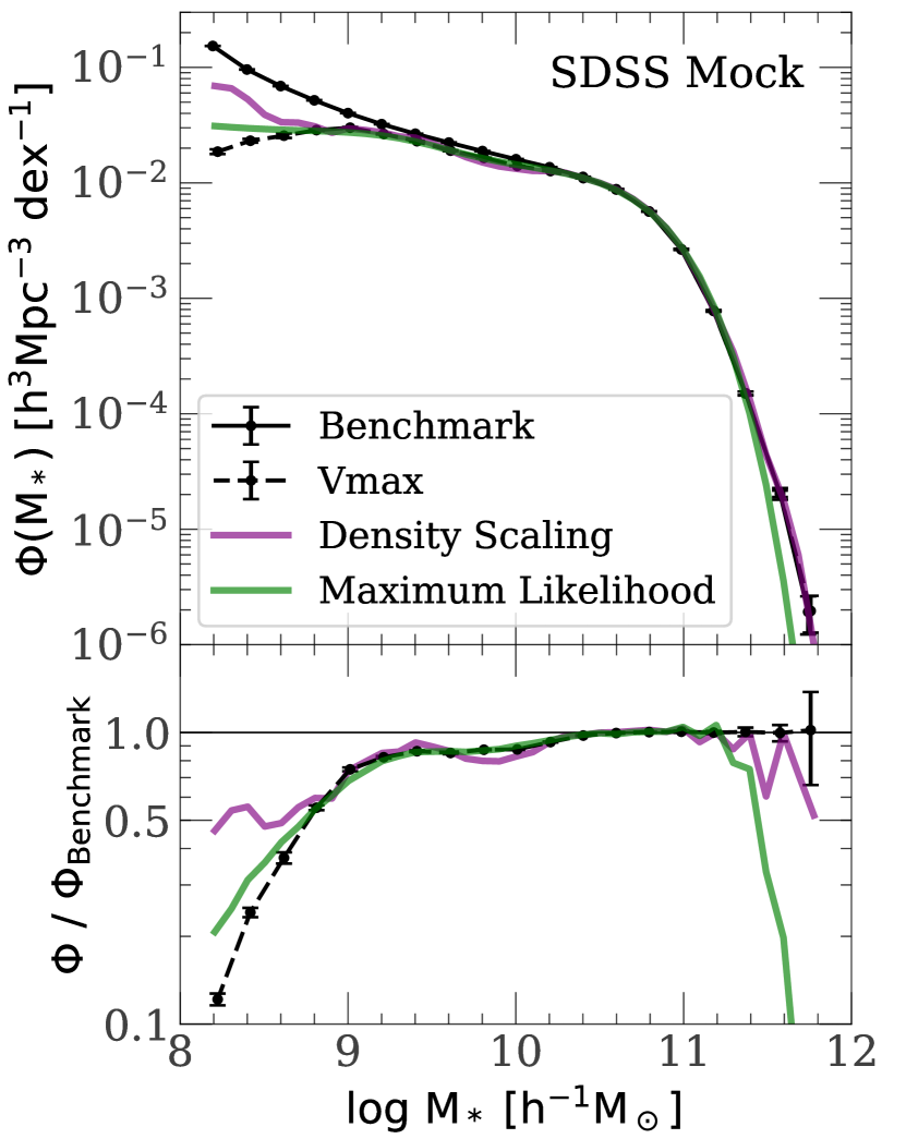
Figure 11.— The GSMFs estimated from the SDSS mock catalog with different methods designed to account for the cosmic variance. Upper panel shows the GSMFs and lower panel shows the ratio of each GSMF to the benchmark. Black solid line: the benchmark GSMF obtained from the SDSS volume-limited mock sample. Black dashed line: the GSMF obtained with the V-max method, with error bars calculated using 100 bootstrap samples. Purple line: the GSMF obtained from the density scaling method of Baldry et al. (2012). Green line: the GSMF obtained from the maximum likelihood method assuming a triple-Schechter function form.

In this subsection we examine in detail the CV in the SDSS using the mock samples constructed for the SDSS. Here we only consider galaxies and model galaxies in the SDSS Northern-Galactic-Cap (NGC) (thereafter, SDSS sky coverage) with redshift $0.01\leq z\leq 0.12$ (thereafter, SDSS volume). We construct four different types of samples：

1. SDSS sample: SDSS DR7 observed galaxies in the SDSS volume, with $r$-band magnitude selection $r\leq 17.6$.

2. SDSS mock sample: model galaxies in the SDSS volume, with r-band magnitude selection $r\leq 17.6$.

3. SDSS magnitude-limited mock samples: model galaxies, in the SDSS volume, that are brighter than a given magnitude limit.

4. SDSS volume-limited mock sample: all model galaxies in the SDSS volume. This sample is served as the benchmark of the GSMF, since it is almost free of cosmic variance, as compared with the entire simulation box.

To investigate potential cosmic variance in the SDSS volume, we first examine the galaxy number density, $n_{g}$, as a function of redshift $z$, in the SDSS volume-limited mock sample. Model galaxies in a given stellar mass bin are binned in redshift intervals with bin size $\delta z=0.005$, and the galaxy count in each bin is used to estimate the galaxy number density. The results are shown in Fig. 9. The redshift distribution of model galaxies in the SDSS volume shows two peaks, one around $z_{1}\approx 0.03$, due to the presence of the large-scale structure known as the CfA Great Wall (Geller & Huchra, 1989), and the other around $z_{2}\approx 0.075$ due to the presence of the the Sloan Great Wall (Gott III et al., 2005). Below $z\approx 0.03$, the number densities show a sharp decline as $z$ decreases, and the effect is stronger for massive galaxies, indicating the presence of a local void (see also, for example Whitbourn & Shanks, 2014, 2016). For comparison, we also show the redshift distribution of SDSS galaxies, obtained by using sub-samples complete to given absolute magnitude limits. We see that the observed distribution follows well that in the mock sample, indicating our mock sample can be used to study the CV in the SDSS sample. For reference we also plot the number densities of simulated dark matter halos in the SDSS volume versus redshift. Here again we see structures similar to that seen in the galaxy distribution. In particular, there is a marked decline of halo density at $z<0.03$, and the decline is more prominent for more massive halos.

The presence of the local low-density region shown above can have strong impact on the statistical properties of the galaxy population derived from the SDSS, especially for faint galaxies which can be observed only within the local volume in a magnitude limited sample. Indeed, the measurement of the GSMF, which describes the number density of galaxies as a function of galaxy mass, can be biased if the local low-density region is not properly accounted for.

As an illustration, Fig. 10 shows the GSMFs derived from SDSS magnitude-limited mock samples with different $r$-band magnitude limits, using the standard $V_{\rm max}$ method. For reference, we also plot the GSMF obtained from the SDSS volume-limited mock sample (the thick dashed line), which matches well the ‘global’ GSMF obtained from the whole $500^{3}\ h^{-3}\mathrm{Mpc}^{3}$ simulation box. As one can see, the GSMF can be significantly underestimated if the magnitude limit is shallow (corresponding to a low value of the $r$-band magnitude limit, $r_{\rm lim}$). Only a sample as deep as $r_{\rm lim}=20$ can provide an unbiased estimate of the GSMF down to $M_{*}\sim 10^{8}\,h^{-1}{\rm M_{\odot}}$. For the SDSS limit, $r_{\rm lim}=17.6$, the measurement starts to deviate from the global GSMF at $M_{*}\approx 10^{9}\,h^{-1}{\rm M_{\odot}}$, and the difference between them reaches a factor of about 5 at around $10^{8}\,h^{-1}{\rm M_{\odot}}$.

The underestimate of the GSMF at the low-mass end is produced by the presence of the low-density region at $z<0.03$ in the SDSS volume. To show this more clearly, we define a ‘break’ mass, $M_{0.03}(r_{\rm lim})$, so that galaxies with stellar masses $M_{*}=M_{0.03}$ is complete to $z=0.03$ for the given magnitude limit, $r_{\rm lim}$. Here we have used the mean mass-to-light ratio, obtained from the mock sample, to convert the stellar mass to an absolute magnitude. As one can see, for each $r_{\rm lim}$, the GSMF obtained from the sample starts to deviate from the global benchmark at $M_{0.03}(r_{\rm lim})$, shown by the vertical line, and is substantially lower at $M_{*}<M_{0.03}$. All these demonstrate that the faint-end of the GSMF can be under-estimated significantly in the SDSS due to the presence of the local low-density region at $z<0.03$.

4.3. The correction of cosmic variance

4.3.1 Conventional methods

The results described above indicate that CV is a serious issue in the measurements of the GSMF, even for a sample as large as the SDSS. Corrections have to be made in order to obtain an unbiased result that represents the true GSMF in the low-$z$ Universe. In the literature, some estimators other than the standard V-max method have been proposed, such as the maximum likelihood method (e.g. G. Efstathiou, 1988; Blanton et al., 2001; Cole, 2011; Whitbourn & Shanks, 2016), and scaling with bright galaxies (e.g. Baldry et al., 2012). These methods were designed, at least partly, to correct for the effects of large-scale structure in the measurements of the GSMF from an observational sample. Here we test their performances using our SDSS mock samples.

In the maximum likelihood method, one starts with an assumed functional form, either parametric or non-parametric, for the GSMF, and then use a maximum likelihood method to match the model prediction with the data, thereby obtaining the parameters that specifies the functional form of the GSMF. In our analysis here, we choose a triple-Schechter function to model the GSMF,

$$\Phi(M_{*})\mathrm{d}\log M_{*}=\sum_{k=1}^{3}\Phi_{*,k}\left(\frac{M_{*}}{\mu_{i}}\right)^{\alpha_{i}+1}e^{-M_{*}/\mu_{i}}{\rm d}\log M_{*}\,,$$ (14)

where $\Phi_{*,i}$, $\mu_{i}$, $\alpha_{i}$ are the amplitude, the characteristic mass, and the faint-end slope, of the $i$-th Schechter component, respectively. This function is assumed to be defined over the domain, $[M_{*,\rm min},\ M_{*,\rm max}]$. For a galaxy, ‘$i$’, with stellar mass $M_{i}$ at redshift $z_{i}$ in the sample, the probability for it to be observed at this redshift is

$${\cal L}_{i}=\frac{\Phi(M_{i})}{\int_{M_{i,\rm min}}^{M_{\rm max}}\Phi(M_{*})\mathrm{d}\log M_{*}}\,.$$ (15)

The total likelihood ${\cal L}$ that the GSMF takes the assumed $\Phi$ is then given by

$${\cal L}=\prod_{i=1}^{N}{\cal L}_{i}\,,$$ (16)

where $N$ is the number of galaxies in the sample. The model parameters can be adjusted so as to maximize the likelihood ${\cal L}$. In our application to the SDSS mock sample, we fit the GSMF obtained from the V-max method with the Triple-Schechter function and use the parameters as the initial input of the maximization process. Since the bright end is free of cosmic variance, we fix the three parameters characterizing the Schechter component at the brightest end, leaving the remaining six parameters to be constrained by the maximum likelihood process. As the maximum likelihood method does not provide information about the overall amplitude of $\Phi(M_{*})$, the bright end is also used to fix the amplitude of $\Phi(M_{*})$. The GSMF estimated in the way from the SDSS mock sample is plotted in Fig. 11 as the green line, in comparison with that estimated by the V-max method (dashed line), and the benchmark GSMF (black line). It is clear that the maximum likelihood method works better than the V-max method, but it still underestimates the GSMF at the low-mass end. The underlying assumption of the maximum likelihood method is that the relative distribution of galaxies with respect to $M_{*}$ is everywhere the same. This in general is not true, given that galaxy clustering depends on $M_{*}$. This explains the failure of this method in correcting the CV.

In an attempt to control the cosmic variance in the GAMA survey, Baldry et al. (2012) proposed to use the number density of brighter galaxies estimated in a larger volume to scale the number density of fainter galaxies that are observed only in a smaller volume. This method will be referred to as “density scaling” method. Our implementation of this method is as follows.

1. Choose a ‘cosmic-variance-free (CVF)’ sample, including only bright galaxies that have $z_{\rm max}$ larger than $0.12$. In our SDSS mock sample, this corresponds to select galaxies with $M_{*}>3\times 10^{10}\,h^{-1}{\rm M_{\odot}}$. This sample will be used as the density tracer at different redshifts, to scale the density at the fainter end.

2. Compute the cumulative number density of the CVF sample, $n_{\rm CVF}(<z)$, as a function of redshift $z$. In practice, the cumulative number density is calculated in the redshift range $[0.01,\ z]$.

3. Compute the GSMF, $\Phi_{\rm Vmax}(M_{*})$, using the V-max method

4. For each stellar mass bin of $\Phi_{\rm Vmax}(M_{*})$, find the largest redshift, $z_{\rm max}(M_{*})$, below which galaxies in this bin can be observed in the sample.

5. Obtain the corrected GSMF, $\Phi_{\rm sc}$, by scaling the V-max estimate with a correction factor:

   $$\Phi_{\rm sc}(M_{*})=\Phi_{\rm Vmax}(M_{*})\frac{n_{\rm CVF}(<0.12)}{n_{\rm CVF}[<z_{\rm max}(M_{*})]}\,,$$ (17)

   where $n_{\rm CVF}(<0.12)$ is the number density of the CVF sample in the full redshift range, $[0.01,0.12]$, and $n_{\rm CVF}[<z_{\rm max}(M_{*})]$ is that in the redshift range $[0.01,z_{\rm max}(M_{*})]$.

The GSMF estimated in this way from the SDSS mock sample is plotted in Fig. 11 as the purple line. This method appears to work better than both the V-max method and the maximum likelihood method in the low-mass end, but the underestimation is still substantial. Furthermore, this method leads to a dip around $M_{*}=10^{9.8}\,h^{-1}{\rm M_{\odot}}$, because of the density enhancement associated with the CfA Great Wall. The failure of this scaling method has an origin similar to that of the maximum likelihood method. The underlying assumption here is that the bright galaxies can serve as a tracer of the cosmic density field, and that the distributions of bright and faint galaxies are both related to the underlying density field by a similar bias factor. In general, this assumption is not valid.

4.3.2 Methods based on the joint distribution of galaxies and environment

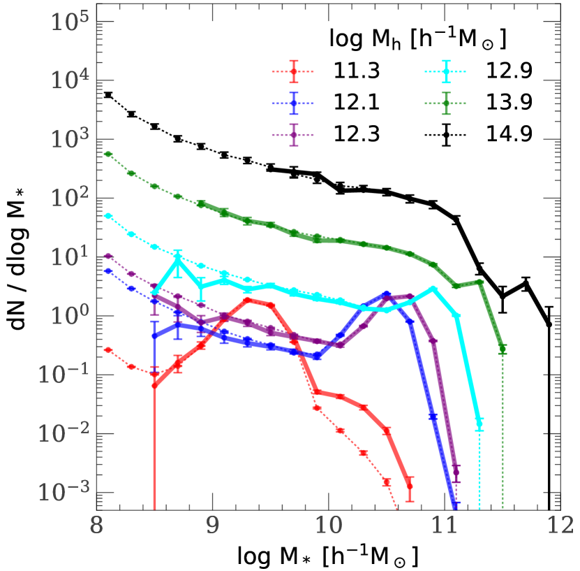
Figure 12.— The conditional galaxy stellar mass functions (CGSMFs) for halos of different masses, $M_{\rm h}$, as indicated in the figure. Solid lines represent the CGSMFs estimated from the SDSS mock sample. Dotted lines are estimated from the SDSS volume-limited mock sample.

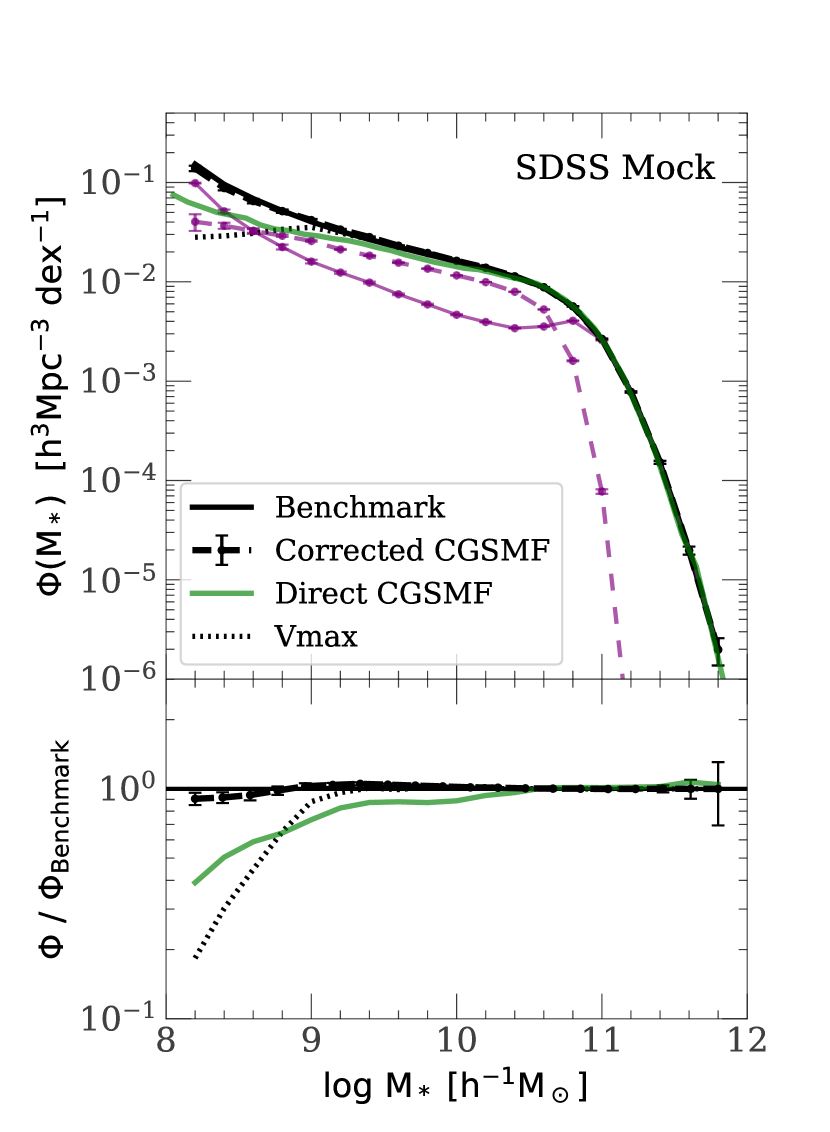
Figure 13.— The GSMFs obtained by applying different methods to the SDSS mock sample. Upper panel shows the GSMFs while the lower panel shows the ratio of each GSMF to the benchmark. Black solid line shows the benchmark GSMF directly calculated from the SDSS volume-limited mock sample. Black dashed line is the GSMF obtained by the method based on the CGSMFs described in this paper. Black dotted line shows the GSMF derived by using the V-max method. Green line shows the GSMF obtained by combining the CGSMFs directly calculated from the SDSS mock sample (which is incomplete for faint galaxies in massive groups). The purple solid and dashed lines are $\Phi_{1}$ and $\Phi_{2}$, the contributions of halos with masses $M_{\rm h}\geq 10^{12.5}\,h^{-1}{\rm M_{\odot}}$ and $M_{\rm h}<10^{12.5}\,h^{-1}{\rm M_{\odot}}$, respectively (see §4.3.2 for details). Error bars are calculated from 100 bootstrap samples.

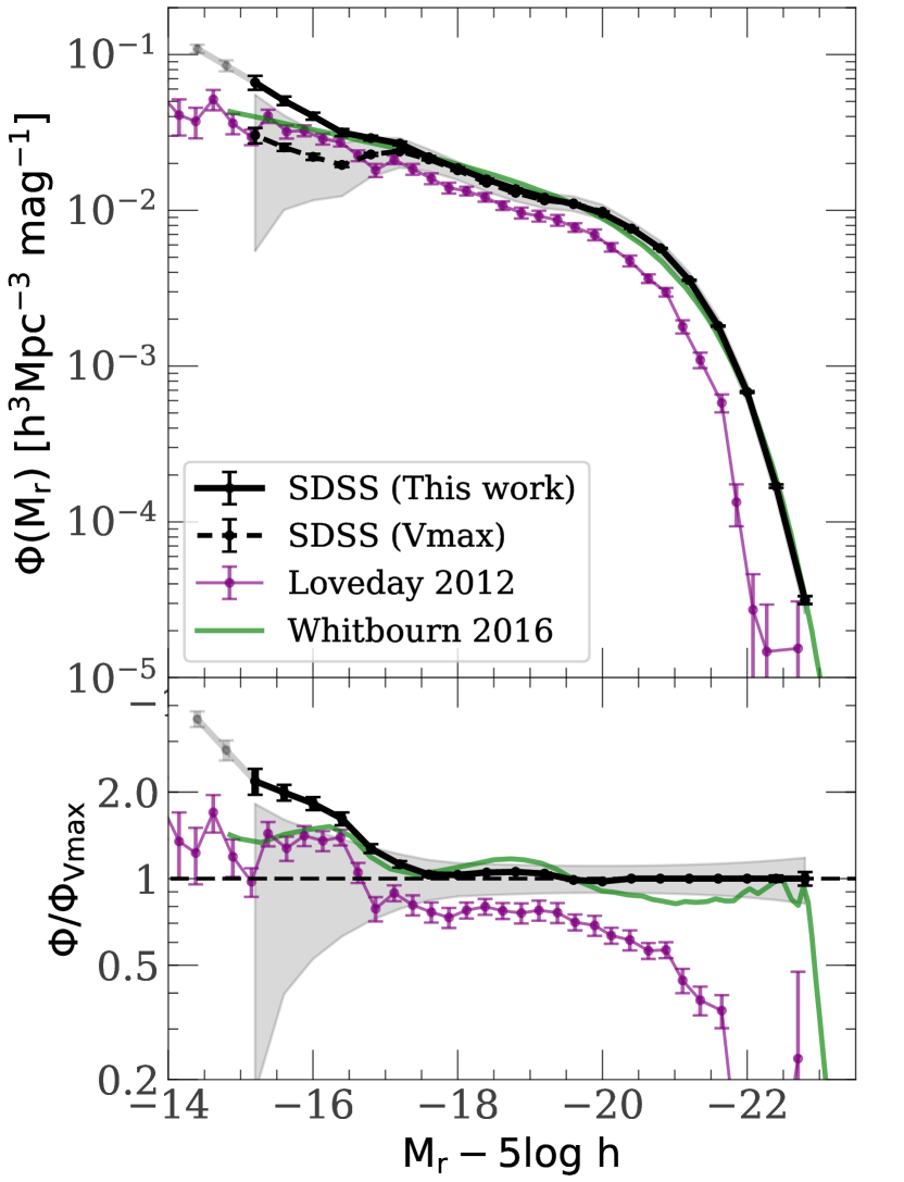
Figure 14.— The galaxy luminosity function (GLF) estimated from the SDSS catalog by using our method, in comparison to the results in the literature. The upper panel shows the GLFs, while the lower panel shows the ratio of each GLF to that obtained with the V-max method. The black solid line is the GLF obtained by our method. The gray solid line at the faint end (first two data points) are obtained by linear extrapolation. Black dashed line is the GLF by the V-max method. The gray shaded band indicates the cosmic variance of SDSS sample expected from Eq. 10. Purple line is from Loveday et al. (2012) for GAMA survey. Green line is from Whitbourn & Shanks (2016) using SDSS ’cmodel’ magnitude.

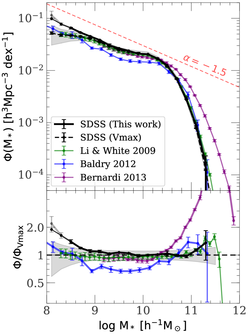
Figure 15.— The galaxy stellar mass function (GSMF) obtained from the SDSS sample in this paper, in comparison with the results published earlier. Upper panel shows the GSMFs, while lower panel shows the ratio of each GSMF to that given by the V-max method. Black solid line is the GSMF obtained by our method. Black dashed line is the GSMF by the V-max method for the SDSS sample. The gray shaded band indicates the cosmic variance of SDSS sample expected from Eq. 10. The gray solid piece at the faint end indicates the slight change when the extrapolation of the GLF is used. Green line: GSMF from Li & White (2009). Blue line: GSMF from the GAMA survey (Baldry et al., 2012). Purple line: GSMF from Bernardi et al. (2013), where the stellar masses of bright galaxies are estimated from Sérsic-Exponential fitting. The red dashed line in the top of upper panel has a slope $\alpha=-1.5$ (see Eq. 14 for the definition of faint-end slope).

Table 1Corrected galaxy luminosity and stellar mass function

$M_{\rm r}-5\log h$	$\log\Phi(M_{\rm r})$	$\log M_{*}$	$\log\Phi(M_{*})$
	$[h^{3}{\rm Mpc}^{-3}{\rm mag}^{-1}]$	$[h^{-1}{\rm M_{\odot}}]$	$[h^{3}{\rm Mpc}^{-3}{\rm dex}^{-1}]$
$-15.2$	$-1.179^{+0.043}_{-0.047}$	$8.1$	$-1.005$	$-0.941$
$-15.6$	$-1.296^{+0.027}_{-0.028}$	$8.3$	$-1.111$	$-1.111$
$-16.0$	$-1.395^{+0.022}_{-0.023}$	$8.5$	$-1.184^{+0.011}_{-0.022}$
$-16.4$	$-1.500^{+0.022}_{-0.023}$	$8.7$	$-1.272^{+0.003}_{-0.008}$
$-16.8$	$-1.536^{+0.015}_{-0.016}$	$8.9$	$-1.345^{+0.007}_{-0.018}$
$-17.2$	$-1.571^{+0.011}_{-0.011}$	$9.1$	$-1.417^{+0.001}_{-0.015}$
$-17.6$	$-1.659^{+0.009}_{-0.009}$	$9.3$	$-1.518^{+0.026}_{-0.009}$
$-18.0$	$-1.730^{+0.006}_{-0.007}$	$9.5$	$-1.576^{+0.002}_{-0.003}$
$-18.4$	$-1.802^{+0.006}_{-0.006}$	$9.7$	$-1.624^{+0.000}_{-0.005}$
$-18.8$	$-1.864^{+0.005}_{-0.005}$	$9.9$	$-1.678^{+0.026}_{-0.013}$
$-19.2$	$-1.919^{+0.004}_{-0.004}$	$10.1$	$-1.688^{+0.004}_{-0.008}$
$-19.6$	$-1.960^{+0.003}_{-0.003}$	$10.3$	$-1.770^{+0.000}_{-0.005}$
$-20.0$	$-2.019^{+0.002}_{-0.002}$	$10.5$	$-1.903^{+0.022}_{-0.030}$
$-20.4$	$-2.117^{+0.002}_{-0.002}$	$10.7$	$-2.163^{+0.010}_{-0.007}$
$-20.8$	$-2.244^{+0.002}_{-0.002}$	$10.9$	$-2.562^{+0.058}_{-0.016}$
$-21.2$	$-2.449^{+0.003}_{-0.003}$	$11.1$	$-3.053^{+0.049}_{-0.012}$
$-21.6$	$-2.743^{+0.004}_{-0.004}$	$11.3$	$-3.770^{+0.131}_{-0.040}$
$-22.0$	$-3.166^{+0.006}_{-0.006}$
$-22.4$	$-3.770^{+0.011}_{-0.011}$
$-22.8$	$-4.501^{+0.023}_{-0.024}$

• Galaxy brighter than $M_{\rm r}-5\log h=-15$ is not sufficient to calculate GSMF down to $M_{*}=10^{8.1},\ 10^{8.3}\,h^{-1}{\rm M_{\odot}}$. Extrapolation of GLF is used to solve this. Left column of $\Phi(M_{*})$ is without extrapolation, while right column is with extrapolation.

Since galaxies form and reside in the cosmic density field, the number density of galaxies is expected to depend on the local environment of galaxies. Suppose the local environment is specified by a quantity or a set of quantities ${\cal E}$. The joint distribution of galaxy mass and ${\cal E}$ obtained from a given sample, ‘$S$’, can be written as

$$\Phi_{S}(M_{*},{\cal E})=\Phi_{S}(M_{*}|{\cal E})P_{S}({\cal E}),$$ (18)

where $\Phi_{S}(M_{*}|{\cal E})$ is the conditional distribution of galaxy mass in a given environment estimated from sample ’S’, and $P_{S}({\cal E})$ is the probability distribution function of the environmental quantity given by the sample. If galaxy formation and evolution is a local process so that $\Phi(M_{*}|{\cal E})$ is independent of the galaxy sample, then the CV in the stellar mass function derived from the sample can all be attributed to the difference between $P_{S}({\cal E})$ and the global distribution function, $P({\cal E})$, expected from a large sample where the distribution of ${\cal E}$ is sampled without bias. An unbiased estimate of the GSMF $\Phi(M_{*})$ is then

$$\Phi(M_{*})=\int\Phi_{S}(M_{*}|{\cal E})P({\cal E})d{\cal E}\,.$$ (19)

Thus, the unbiased GSMF is obtained from the conditional distribution function, $\Phi_{S}(M_{*}|{\cal E})$, derived from the sample ‘$S$’, and the unbiased distribution $P({\cal E})$ of environment variable.

The environmental quantity has to be chosen properly so that it can be estimated from observation, while the unbiased distribution function, $P({\cal E})$, can, in principle, be obtained from large cosmological simulations. Here we analyze a method which uses the masses of dark matter halos as the environmental quantity. In this case, ${\cal E}$ is represented by halo mass, $M_{\rm h}$, $\Phi_{S}(M_{*}|M_{\rm h})$ is the conditional galaxy stellar mass function(CGSMF), and $P({\cal E})=n(M_{\rm h})$ is the halo mass function estimated directly from the constrained simulation (Yang et al., 2003). The advantage here is that the unbiased estimates are only needed for the conditional functions, $\Phi(M_{*}|M_{\rm h})$. The disadvantage is that it is model dependent through $n(M_{\rm h})$, and that one has to identify galaxy systems to represent dark matter halos.

Fig. 12 shows the conditional stellar mass functions, of galaxies in halos of different masses, estimated from the SDSS mock sample, in comparison with the benchmarks obtained from the total SDSS volume-limited sample. As one can see, for a given halo mass, the CGSMF obtained from the SDSS mock sample matches the benchmark well only in the massive end. This happens because of the absence of massive halos at small distances in the local under-dense region, so that their faint member galaxies are not observed in the magnitude limited sample. The total GSMF, obtained using Eq. (19), is shown in the Fig. 13 by the green line, in comparison to the benchmark of the total GSMF represented by the black solid line, and to the GSMF obtained by the traditional V-max method represented by the black dotted line. Here the benchmark CGSMFs (dotted lines in Fig. 12) are used for halos with $M_{\rm h}<10^{12}\,h^{-1}{\rm M_{\odot}}$, while the CGSMFs estimated from the magnitude-limted sample (solid lines in Fig. 12) are used for less massive halos. This is to mimic the fact that the total CGSMF for less massive halos can be obtained by other means (see Eq. 21), while the low-stellar-mass end of CMGSFs for massive halos cannot be obtained directly from the SDSS spectroscopic sample. Here again the stellar mass function at the low-mass end is under-estimated, although the method works substantially better than the V-max method. The reason is clear from Fig. 12. The stellar mass function at the low mass end is only sampled by low-mass halos because of the absence of massive halos in the nearby volume, while the low-mass end in the benchmark stellar mass function is actually affected by the low-mass ends of the conditional stellar mass functions of massive halos.

These results demonstrate an important point. If the shape of the CGSMF depends significantly on halo mass, then one needs to estimate all the conditional functions reliably down to a given stellar mass limit, in order to get an unbiased estimate of the total stellar mass function down to the same mass limit. The SDSS redshift sample is clearly insufficient to achieve this goal in the low-mass end.

In a recent paper, Lan et al. (2016) showed that the conditional functions of galaxies can be estimated down to $M_{r}\sim-14$ (corresponding to a stellar mass of about $10^{8}{\rm M_{\odot}}$) for halos with mass $M_{\rm h}>10^{12}{\rm M_{\odot}}$ by cross correlating galaxy groups (halos) selected from the SDSS spectroscopic sample with SDSS photometric data. Thus, if we can estimate the contribution by halos with lower masses to a similar magnitude, then the total function can be obtained. Here we test the feasibility of such an approach using SDSS mock sample. First, we obtain the CGSMFs down to a stellar mass of $10^{8}\,h^{-1}{\rm M_{\odot}}$ for halos with $M_{\rm h}\geq M_{1}=10^{12.5}\,h^{-1}{\rm M_{\odot}}$ directly from the total simulation volume. This step is to mimic the fact that such CGSMFs can be obtained, as in Lan et al. (2016), from observational data. The GSMF contributed by such halos is

$$\Phi_{1}(M_{*})=\int_{M_{1}}^{\infty}\Phi(M_{*}|M_{\rm h})n(M_{\rm h})dM_{\rm h}\,,$$ (20)

To maximally reduce possible uncertainties introduced by this procedure, we estimate the total CGSMF $\Phi_{1}$ for $M_{\rm h}\geq M_{1}$ directly from a modified V-max method for the high-stellar-mass end. Specifically, each galaxy is assigned a weight, $n_{\rm halo,u}/n_{\rm halo}(V_{\rm max})$, the ratio between the number density of $M_{\rm h}\geq M_{1}$ halos in the Universe and that in $V_{\rm max}$. In practice, the weighted V-max has little impact on the results, as the effect of cosmic variance for high-mass galaxies is small. The procedure is included only for maintaining consistency. Eq. (20) is then used only at the low-stellar-mass end where the V-max method fails because of incompleteness. The result for $\Phi_{1}$ obtained in this way is shown by the purple solid curve in Fig 13.

To estimate the contribution by halos with $M_{\rm h}<M_{1}$ in a way that can be applied to real observation, we first eliminate all galaxies that are contained in halos with $M_{\rm h}\geq M_{1}$. For the rest of the galaxies, we estimate the function by a modified version of the V-max method

$$\Phi_{2}(M_{*})=\sum{\frac{1}{V_{\rm max}}}\frac{1}{1+b\delta(V_{\rm max})}\,,$$ (21)

where the summation is over individual galaxies, $b=0.6$ is the bias factor which is considered to be constant for low-mass halos (e.g. Sheth et al., 2001), $\delta(V_{\rm max})={{\overline{\rho}}(V_{\rm max})/\rho_{\rm u}}-1$ is the mean over density within $V_{\rm max}$, $\rho_{\rm u}$ is the universal mass density, and ${\overline{\rho}}(V_{\rm max})$ is the mean mass density within $V_{\rm max}$. The function $\Phi_{2}$ so estimated is shown as the purple dashed curve in Fig.13. Note that small groups can only be seen in the very local region, so the CGSMF estimated for halos in a small mass bin can be very noisy. Our method intends to avoid this uncertainty by calculating the total CGSMF for all halos less massive than $M_{1}$. The total GSMF, $\Phi=\Phi_{1}+\Phi_{2}$ is shown by the black dashed line in Fig.13, which is very close to the benchmark, indicating that our method can indeed take care of the bias produced by the local under-dense region. We have checked that the result depends only weakly on the choice of the value of $M_{1}$.

4.4. Applications to observational data

In this subsection, we apply the method described above to the real SDSS sample. We first estimate the galaxy luminosity function (GLF) using the procedure based on the conditional distributions of galaxy luminosity in dark matter halos, as described in §4.3.2. Here the CLF, $\Phi_{1}(M_{r})$, for faint galaxies with magnitude $M_{r}-5\log h>-17.2$ in halos more massive than $10^{12.5}\,h^{-1}{\rm M_{\odot}}$ are obtained from Lan et al. (2016), while the CLF for brighter galaxies in these halos is estimated directly from SDSS sample using the V-max method and the group catalog of Yang et al. (2012) (see also Yang et al., 2007). For halos with masses below $10^{12.5}\,h^{-1}{\rm M_{\odot}}$ the CLF, $\Phi_{2}(M_{r})$, is obtained from the SDSS sample using the modified V-max method as described by Eq. (21). The total galaxy luminosity function (GLF) is then obtained by $\Phi(M_{r})=\Phi_{1}(M_{r})+\Phi_{2}(M_{r})$. Fig. 14 shows the result of the GLF so obtained in solid black line, in comparison with that obtained from the traditional V-max method. At the faint end, $M_{r}-5\log h\approx-15$, the GLF is about twice as high as that given by the V-max method, indicating that cosmic variance can have large impact on the estimate of the GLF at the faint end. To show this more clearly, we plot the cosmic variance expected from Eq. 10 as the shaded band in Fig. 14, where the stellar mass is obtained from luminosity by using mean mass-to-light ratio. The expected cosmic variance is quite large at the faint end, indicating that cosmic variance is an important issue in estimating the faint end of GLF. The GLF in the local Universe has been estimated by many authors using various samples (e.g. Blanton et al., 2003; Yang et al., 2009; Loveday et al., 2012; Jones et al., 2006; Driver et al., 2012; Whitbourn & Shanks, 2016). For comparison, we plot the GLFs obtained by Loveday et al. (2012) from the GAMA survey and by Whitbourn & Shanks (2016), who applies a maximum likelihood method to the SDSS to account for the cosmic variance in their estimates. The result of Whitbourn & Shanks (2016) matches ours over a wide range of luminosity, but seems to still underestimate the GLF at the faint end. The result of Loveday et al. (2012) has a large discrepancy with our result, possibly due to the cosmic variance in the small sky converage of the GAMA sample used, which is $144\deg^{2}$. Since many of the faint galaxies in the SDSS photometric data do not have reliable stellar mass estimates, conditional galaxy stellar mass functions are not available at the low mass end. Because of this, we cannot estimate the GSMF down to the low-mass end directly from the data with the method above. As an alternative, we use the $M_{r}$ - $M_{*}$ relation obtained from the SDSS spectroscopic sample to convert the GLF obtained above to estimate a GSMF. We do this through the following steps. (i) Construct a large volume-limited Monte-Carlo sample of galaxies with absolute magnitude distribution given by the GLF. (ii) Bin these galaxies according to their absolute magnitudes. (iii) For each Monte-Carlo galaxy, we randomly choose a galaxy in the real SDSS spectroscopic sample in the same absolute magnitude bin, and assign the stellar mass of the real galaxy to the Monte Carlo galaxy. (iv) Compute the GSMF of this volume-limited Monte-Carlo sample.

The GSMF obtained directly from the GLF in this way is shown in Fig. 15 by the black solid curve. Since the GLF is estimated only down to $M_{r}-5\log h\approx-15$, the first two data points in the low-mass end of the GSMF may be underestimated, as galaxies fainter than $M_{r}-5\log h=-15$ may contribute to these two stellar mass bins. To test this, we extrapolate the faint end of the GLF to $M_{r}-5\log h=-14.2$, which is sufficient to include all galaxies with stellar masses down to $10^{8}\,h^{-1}{\rm M_{\odot}}$. This extrapolation is shown by the gray extension of the black solid curve in Fig. 14. The GSMF obtained from the extended GLF is shown by the gray line in Fig.15. As one can see, the extension of the GLF only slightly increases the GSMF at the lowest mass. The GSMF estimated in this way is compared with that estimated with the conventional V-max method. The gray shaded band shows the expected cosmic variance given by Eq. 10 for the SDSS sample. The effect of CV is quite large at the low-stellar-mass end. The difference between our result and that obtained from the V-max method is even larger, indicating again that the local SDSS region is an unusually under-dense region. The GSMF in the low-$z$ Universe has been estimated in numerous earlier investigations using different samples and methods (e.g. Li & White, 2009; Yang et al., 2009; Baldry et al., 2012; Bernardi et al., 2013; He et al., 2013; D’Souza et al., 2015). Several of the earlier results are plotted in Fig. 15 for comparison. The result of Li & White (2009), who measured the GSMF of SDSS sample directly from the stellar masses estimated by Blanton & Roweis (2007) with a Chabrier IMF (Chabrier, 2003) and corrections for dust, matches well our V-max result, and also misses the steepening of the GSMF at $M_{*}<10^{9.5}\,h^{-1}{\rm M_{\odot}}$. Our measurement at $M_{*}>10^{10.5}\,h^{-1}{\rm M_{\odot}}$ is significantly lower than that from Bernardi et al. (2013), because they included the light in the outer parts of massive galaxies that may be missed in the SDSS NYU-VAGC used here (see also He et al. 2013 for the discussion of this effect). Such corrections do not affect the GSMF in the low-mass end. The overall shape of our GSMF is similar to that of Baldry et al. (2012) obtained from the GAMA sample, but the amplitude of their function is about $50\%$ lower. GAMA has a small sky coverage, $144\deg^{2}$, although it is deeper, to $r\approx 19.8$. According to our test with mock samples of a similar sky coverage and depth, the cosmic variance in the GSMF estimated from such a sample can be very large. The lower amplitude given by the GAMA sample may be produced by such cosmic variance.

In conclusion, when CV is carefully taken into account, the low-stellar-mass end slope of the GSMF in the low-$z$ Universe, which is about $-1.5$ as indicated by the red dashed line in Fig. 15, is significantly steeper than those published in earlier studies. In particular, there is a significant upturn at $M_{*}<10^{9.5}\,h^{-1}{\rm M_{\odot}}$ in the GSMF that is missed in many of the earlier measurements. For reference, we list the GLF and GSMF estimated with our method in Table 1.

5. Summary and discussion

In this paper, we use ELUCID simulation, a constrained $N$-body simulation in the Sloan Digital Sky Survey (SDSS) volume to study galaxy distribution in the low-$z$ Universe. Our main results can be summarized as follows:

1. Dark matter halos are selected from different snapshots of the simulation, and halo merger trees are constructed from the simulated halos down to a halo mass of $\sim 10^{10}\,h^{-1}{\rm M_{\odot}}$. A method is developed to extend all the simulated halo merger trees to a mass resolution of $10^{9}\,h^{-1}{\rm M_{\odot}}$, which is needed to model galaxies down to a stellar mass of $10^{8}\,h^{-1}{\rm M_{\odot}}$.

2. The merger trees are used to populate simulated dark matter halos with galaxies according to an empirical model of galaxy formation developed by Lu et al. (2014b); Lu et al. (2015a). The model galaxies follow the real galaxies in the SDSS volume both in spatial distribution and in intrinsic properties. The catalog of the model galaxies, therefore, provide a unique way to study galaxy formation and evolution in the cosmic web in the low-$z$ Universe.

3. Mock catalogs in the SDSS sky coverage are constructed, which can be used to investigate the distribution of galaxies as measured from the real SDSS data and its relation to the global distribution expected from a fair sample of galaxies in the low-$z$ Universe. These mock catalogs can thus be used to quantify the cosmic variances in the statistical properties of the low-$z$ galaxy population estimated from a survey like SDSS.

4. As an example, we use the mock catalogs so constructed to quantify the cosmic variance in the galaxy stellar mass function (GSMF). Useful fitting formulae are obtained to describe the cosmic variance and covariance matrix of the GSMF as functions of stellar mass and sample volume.

5. We find that the GSMF estimated from the SDSS magnitude-limited sample can be affected significantly by the presence of the under-dense region at $z<0.03$, so that the low-mass end of the function can be underestimated significantly.

6. We test several existing methods that are designed to deal with the effects of the cosmic variance in the estimate of GSMF, and find that none of them is able to fully account for the cosmic variance effects.

7. We propose and test a method based on the conditional stellar mass functions in dark matter halos, which is found to provide an unbiased estimate of the global GSMF.

8. We apply the method to the SDSS data and find that the GSMF has a significant upturn at $M_{*}<10^{9.5}\,h^{-1}{\rm M_{\odot}}$, which is missed in many earlier measurements of the local GSMF.

Our results of the GSMF have important implications for galaxy formation and evolution. The presence of an upturn in the GSMF at $M_{*}<10^{9.5}\,h^{-1}{\rm M_{\odot}}$ suggests that there is a characteristic mass scale, $\sim 10^{9.5}\,h^{-1}{\rm M_{\odot}}$, corresponding to a halo mass of $\sim 10^{11}\,h^{-1}{\rm M_{\odot}}$ (e.g. Lim et al., 2017a), below which star formation may be affected by processes that are different from those in galaxies of higher masses. The stellar mass function of galaxies at low-$z$ has been widely used to calibrate numerical simulations and semi-analytic models of galaxy formation. The improved estimate of the GSMF presented here clearly will provide more accurate constraints on theoretical models.

The mock catalogs constructed here have other applications. For example, they can be used to analyze the cosmic variance in the measurements of other statistical properties of the galaxy population, such as the correlation functions (Zehavi et al., 2005; Wang et al., 2007) and peculiar velocities (e.g. Jing et al., 1998; Loveday et al., 2018) of galaxies of different luminosities/masses. Because of the presence of local large-scale structures, such as the under-dense region at $z<0.03$, the measurements for faint galaxies can be affected. A comparison between the results obtained from the mock sample and that from the benchmark sample can then be used to quantify the effects of cosmic variance. Another application is to HI samples of galaxies. Current HI surveys, such as HIPASS (Meyer et al., 2004) and ALFALFA (Giovanelli et al., 2005), are shallow, typically to $z\sim 0.05$, and so the HI-mass functions and correlation functions estimated from these surveys can be affected significantly by the cosmic variance in the nearby Universe (e.g. Guo et al., 2017). The same method as described here can be used to construct mock catalogs for HI galaxies, and to quantify cosmic variances in these measurements. We will come back to some of these problems in the future.

References

- Babul & Rees (1992) Babul A., Rees M. J., 1992, MNRAS, 255, 346
- Baldry et al. (2012) Baldry I. K., et al., 2012, MNRAS, 421, 621
- Bernardi et al. (2013) Bernardi M., Meert A., Sheth R. K., Vikram V., Huertas-Company M., Mei S., Shankar F., 2013, MNRAS, 436, 697
- Blanton & Roweis (2007) Blanton M. R., Roweis S., 2007, AJ, 133, 734
- Blanton et al. (2001) Blanton M. R., et al., 2001, AJ, 121, 2358
- Blanton et al. (2003) Blanton M. R., et al., 2003, ApJ, 592, 819
- Boylan-Kolchin et al. (2008) Boylan-Kolchin M., Ma C.-P., Quataert E., 2008, MNRAS, 383, 93
- Bruzual & Charlot (2003) Bruzual G., Charlot S., 2003, MNRAS, 344, 1000
- Chabrier (2003) Chabrier G., 2003, PASP, 115, 763
- Cole (2011) Cole S., 2011, MNRAS, 416, 739
- D’Souza et al. (2015) D’Souza R., Vegetti S., Kauffmann G., 2015, MNRAS, 454, 4027
- Davis et al. (1985) Davis M., Efstathiou G., Frenk C. S., White S. D. M., 1985, ApJ, 292, 371
- Driver & Robotham (2010) Driver S. P., Robotham A. S. G., 2010, MNRAS, 407, 2131
- Driver et al. (2012) Driver S. P., et al., 2012, MNRAS, 427, 3244
- Dunkley et al. (2009) Dunkley J., et al., 2009, ApJS, 180, 306
- G. Efstathiou (1988) G. Efstathiou 1988, MNRAS, 232, 431
- Gallazzi et al. (2005) Gallazzi A., Charlot S., Brinchmann J., White S. D. M., Tremonti C. A., 2005, MNRAS, 362, 41
- Geller & Huchra (1989) Geller M. J., Huchra J. P., 1989, Sci, 246, 897
- Giovanelli et al. (2005) Giovanelli R., et al., 2005, AJ, 130, 2598
- Gott III et al. (2005) Gott III J. R., Jurić M., Schlegel D., Hoyle F., Vogeley M., Tegmark M., Bahcall N., Brinkmann J., 2005, ApJ, 624, 463
- Guo et al. (2017) Guo H., Li C., Zheng Z., Mo H. J., Jing Y. P., Zu Y., Lim S. H., Xu H., 2017, ApJ, 846, 61
- He et al. (2013) He Y. Q., Xia X. Y., Hao C. N., Jing Y. P., Mao S., Li C., 2013, ApJ, 773, 37
- Jha et al. (2007) Jha S., Riess A. G., Kirshner R. P., 2007, ApJ, 659, 122
- Jiang & van den Bosch (2014) Jiang F., van den Bosch F. C., 2014, MNRAS, 440, 193
- Jing et al. (1998) Jing Y. P., Mo H. J., Borner G., 1998, ApJ, 494, 1
- Jones et al. (2006) Jones D. H., Peterson B. A., Colless M., Saunders W., 2006, MNRAS, 369, 25
- Keenan et al. (2013) Keenan R. C., Barger A. J., Cowie L. L., 2013, ApJ, 775, 62
- Komatsu et al. (2009) Komatsu E., et al., 2009, ApJS, 180, 330
- Lan et al. (2016) Lan T.-W., Ménard B., Mo H., 2016, MNRAS, 459, 3998
- Li & White (2009) Li C., White S. D. M., 2009, MNRAS, 398, 2177
- Lim et al. (2017a) Lim S. H., Mo H. J., Lan T.-W., Ménard B., 2017a, MNRAS, 464, 3256
- Lim et al. (2017b) Lim S. H., Mo H. J., Lu Y., Wang H., Yang X., 2017b, MNRAS, 470, 2982
- Loveday et al. (2012) Loveday J., et al., 2012, MNRAS, 420, 1239
- Loveday et al. (2018) Loveday J., et al., 2018, MNRAS, 474, 3435
- Lu et al. (2014a) Lu Z., Mo H. J., Lu Y., Katz N., Weinberg M. D., van den Bosch F. C., Yang X., 2014a, MNRAS, 439, 1294
- Lu et al. (2014b) Lu Y., Mo H. J., Lu Z., Katz N., Weinberg M. D., 2014b, MNRAS, 443, 1252
- Lu et al. (2015a) Lu Z., Mo H. J., Lu Y., 2015a, MNRAS, 450, 606
- Lu et al. (2015b) Lu Z., Mo H. J., Lu Y., Katz N., Weinberg M. D., van den Bosch F. C., Yang X., 2015b, MNRAS, 450, 1604
- Marra et al. (2013) Marra V., Amendola L., Sawicki I., Valkenburg W., 2013, PRL, 110, 241305
- Meyer et al. (2004) Meyer M. J., et al., 2004, MNRAS, 350, 1195
- Mo & White (1996) Mo H. J., White S. D. M., 1996, MNRAS, 282, 347
- Moster et al. (2011) Moster B. P., Somerville R. S., Newman J. A., Rix H.-W., 2011, ApJ, 731, 113
- Navarro et al. (1997) Navarro J. F., Frenk C. S., White S. D. M., 1997, ApJ, 490, 493
- Parkinson et al. (2008) Parkinson H., Cole S., Helly J., 2008, MNRAS, 383, 557
- Peebles (1980) Peebles P. J. E., 1980, The large-scale structure of the universe. Princeton University Press, Princeton
- Sheth et al. (2001) Sheth R. K., Mo H. J., Tormen G., 2001, MNRAS, 323, 1
- Somerville et al. (2004) Somerville R. S., Lee K., Ferguson H. C., Gardner J. P., Moustakas L. A., Giavalisco M., 2004, ApJ, 600, L171
- Springel (2005) Springel V., 2005, MNRAS, 364, 1105
- Springel et al. (2005) Springel V., et al., 2005, Natur, 435, 629
- Thoul & Weinberg (1996) Thoul A. A., Weinberg D. H., 1996, ApJ, 465, 608
- Wang et al. (2007) Wang Y., Yang X., Mo H. J., van den Bosch F. C., 2007, ApJ, 664, 608
- Wang et al. (2009) Wang H., Mo H. J., Jing Y. P., Guo Y., van den Bosch F. C., Yang X., 2009, MNRAS, 394, 398
- Wang et al. (2013) Wang H., Mo H. J., Yang X., van den Bosch F. C., 2013, ApJ, 772, 63
- Wang et al. (2014) Wang H., Mo H. J., Yang X., Jing Y. P., Lin W. P., 2014, ApJ, 794, 94
- Wang et al. (2016) Wang H., et al., 2016, ApJ, 831, 164
- Whitbourn & Shanks (2014) Whitbourn J. R., Shanks T., 2014, MNRAS, 437, 2146
- Whitbourn & Shanks (2016) Whitbourn J. R., Shanks T., 2016, MNRAS, 459, 496
- Wojtak et al. (2014) Wojtak R., Knebe A., Watson W. A., Iliev I. T., Heß S., Rapetti D., Yepes G., Gottlöber S., 2014, MNRAS, 438, 1805
- Yang et al. (2003) Yang X., Mo H. J., van den Bosch F. C., 2003, MNRAS, 339, 1057
- Yang et al. (2007) Yang X., Mo H. J., van den Bosch F. C., Pasquali A., Li C., Barden M., 2007, ApJ, 671, 153
- Yang et al. (2008) Yang X., Mo H. J., van den Bosch F. C., 2008, ApJ, 676, 248
- Yang et al. (2009) Yang X., Mo H. J., van den Bosch F. C., 2009, ApJ, 695, 900
- Yang et al. (2012) Yang X., Mo H. J., van den Bosch F. C., Zhang Y., Han J., 2012, ApJ, 752, 41
- Zehavi et al. (2005) Zehavi I., et al., 2005, ApJ, 630, 1
- Zentner et al. (2005) Zentner A. R., Berlind A. A., Bullock J. S., Kravtsov A. V., Wechsler R. H., 2005, ApJ, 624, 505
- Zhao et al. (2009) Zhao D. H., Jing Y. P., Mo H. J., Börner G., 2009, ApJ, 707, 354