A Bilevel Approach to Optimal Price-Setting of Time-and-Level-of-Use Tariffs

Summary

Time-and-Level-of-Use (TLOU) is a recently proposed pricing policy for energy, extending Time-of-Use with the addition of a capacity that users can book for a given time frame, reducing their expected energy cost if they respect this self-determined capacity limit. We introduce a variant of the TLOU defined in the literature, aligned with the supplier interest to prevent unplanned over-consumption. The optimal price-setting problem of TLOU is defined as a bilevel, bi-objective problem anticipating user choices in the supplier decision. An efficient resolution scheme is developed, based on the specific discrete structure of the lower-level user problem. Computational experiments using consumption distributions estimated from historical data illustrate the effectiveness of the proposed framework.

Keywords: Demand response, electricity pricing, bilevel optimization, Time-and-Level-of-Use

Introduction

The increasing penetration of wind and solar energy has marked the last decades, bringing a decentralization and higher stochasticity of power generation, yielding new challenges for the operation of electrical grids. Advances in communication technologies have enabled both scheduling of smart appliances and seamless data collection and exchange between different entities operating on power networks, from generators to end-consumers. Using such capabilities, agents can make decisions based on probability distributions of different variables, possibly conditioned on known external factors, such as the weather.

As a promising lead to tackle these challenges, Demand Response (DR) has attracted an increasing interest in the past decades. Instead of compensating ever-increasing fluctuations of renewable production with conventional power generation, this approach consists in leveraging the flexibility of some consuming units by reducing or shifting their load[1]. The Time-and-Level-of-Use system presented in this paper is primarily a price-based Demand Response program based on the classification found in the literature[1], although the self-determined consumption limit creates an incentive for respecting the commitment on the part of the user. Its design makes opting out of the program a natural extension and thus requires less coupling and interaction between users and suppliers to work. In a 2012 report, the US Federal Energy Regulatory Commission identified the lack of short-term estimation methods as one of the critical barriers to the effective implementation of Demand Response [2]. In a related approach[3], an incentive-based Demand Response program is developed with users signaling both a predicted consumption and a reduction capacity, with the supplier selecting reductions randomly. Both the program developed by the authors[3] and the TLOU policy require a signal sent from the user to the supplier.

Bilevel optimization has been used to model and tackle optimization problems in energy networks [4]. Applications on power systems and markets are also mentioned in several reviews on bilevel optimization [5, 6]. It allows decision-makers to encapsulate utility-generators, user-utility interactions [7, 8], or define robust formulations of unit commitment and optimal power flow [9]. Some recent work focuses on bilevel optimization for demand-response in the real-time market [10]. Multiple supplier settings are also considered, for instance in the determination of Time-of-Use pricing policies [11], where competing retailers target residential users.

The Time-and-Level-of-Use (TLOU) pricing scheme [12] was built as an extension of Time-of-Use (TOU), targeting specifically the issue with current large-scale Demand-Response programs identified in the FERC report[2]. The optimal planning and operation of a smart building under this scheme was developed, taking the TLOU settings as input of the decision. In this work, we consider the perspective of the supplier determining the optimal parameters of TLOU.

We integrate the optimal user reaction in the supplier decision problem, thus modelling the interaction as a Stackelberg game solved as a bilevel optimization problem. The specific structure of the lower-level decision is leveraged to reduce the set of possibly optimal solutions to a finite enumerable set. Through this reduction, the lower-level optimality conditions are translated into a set of linear constraints. The set of optimal pricing configurations is derived for different distributions corresponding to different time frames. These options can be computed in advance and then one is chosen by the supplier ahead of the consumption time to create an incentive to book and consume a given capacity. We show the effectiveness of the method with discrete probability distributions computed from historical consumption data.

Time-and-Level-of-Use pricing

The TLOU policy was initially developed from the perspective of smart consumption units[12] which can be a building, an apartment or a micro-grid monitoring its consumption and equipped with programmable consuming devices. It is a pricing model for energy built upon the Time-of-Use (TOU) implemented by several jurisdictions and for which the energy price is fixed by intervals throughout the day. TLOU extends TOU by allowing users to self-determine and book an energy capacity at each time frame depending on their planned requirements; and by doing so, they provide the supplier with information on the intended consumption. We will refer to the capacity as the amount of energy booked by the user for a given time frame, following the same terminology as the reference implementation[12]. Energy prices still depend on the time frame within the day, but also on the capacity booked by the user. This pricing scheme is applied in a three-phase process:

1. The supplier sends the pricing information to the user.

2. The user books a capacity from the supplier for the time frame before a given deadline. If no capacity has been booked, the Time-of-Use pricing is used.

3. After the time frame, the energy cost is computed depending on the energy consumed $x$ and booked capacity $c$:

   • If $x\leq c$, then the applied price of energy is $\pi^{L}(c)$ and the energy cost is $\pi^{L}(c)\cdot x$.

   • If $x>c$, then the applied price of energy is $\pi^{H}(c)$ and the energy cost is $\pi^{H}(c)\cdot x$.

In the model considered in this paper, only the first two steps involve decisions from the agents, making the decision process a Stackelberg game given the sequentiality of these decisions. The price structure is composed of three elements: a booking fee $K$, a step-wise decreasing function $\pi^{L}(c)$ representing the lower energy price and a step-wise increasing function $\pi^{H}(c)$ representing the higher energy price. The steps of the lower and higher price functions are given at different breakpoints:

$$\{c^{L}_{0},c^{L}_{1},c^{L}_{2},...\}=C^{L} \& \,\,\{\pi^{L}_{0},\pi^{L}_{1},\pi^{L}_{2},...\}=\pi^{L}$$

$$\{c^{H}_{0},c^{H}_{1},c^{H}_{2},...\}=C^{H} \& \,\,\{\pi^{H}_{0},\pi^{H}_{1},\pi^{H}_{2},...\}=\pi^{H}$$

$\pi^{L}(c)$ will refer to the function of the capacity and $\pi^{L}_{j}$ to the value of the lower price at step $j$. In the initial version of the pricing [12], the energy consumed above the capacity is paid at the higher tariff while the rest is paid at the lower tariff.

Considering that most power systems try to prevent over-consumption and unplanned excess consumption, we introduce a variant where the whole energy consumed is paid at the lower tariff if it is less or equal to the capacity, and at the higher tariff otherwise, see Equation (1). In other words, if the consumption over the time frame remains below the booked capacity, the effective energy price is given by the lower tariff curve; if the consumption exceeds the booked capacity, the energy price is given by the higher tariff. The total cost for the user associated with a booked capacity $c$ and a consumption $X_{t}$ for a time frame $t$ is:

$$\mathcal{C}(c_{t};X_{t})=\begin{cases}K\cdot c_{t}+\pi^{L}(c_{t})\cdot X_{t},&\mbox{if}\,X_{t}\ \leq\ c_{t},\\ K\cdot c_{t}+\pi^{H}(c_{t})\cdot X_{t}&\mbox{otherwise.}\end{cases}$$ (1)

The load distribution $X_{t}$ is a random variable; both user and supplier make decisions on the expected cost over the set of possible consumption levels $\Omega$, given as:

$$\mathcal{C}(c_{t})=\mathbb{E}_{\Omega}\left[\mathcal{C}(c_{t};x_{\omega})\right]$$ (2)

where $\mathbb{E}_{\Omega}$ is the expected value over the support $\Omega$ of the probability distribution.

Furthermore, $\pi^{L}(c=0)=\pi^{H}(c=0)=\pi_{0}(t)$, with $\pi_{0}(t)$ the Time-of-Use price at the time frame of interest $t$. This property allows users to opt-out of the program for some time frames by simply not booking any capacity. TLOU is designed for the day-ahead market, where both the pricing components and the capacity are chosen ahead of the consumption time [12]. It can however be adjusted to other markets [13] or intra-day settings. The entity defining the TLOU pricing can also extend the possible settings by decoupling the time spans for one price setting choice from the time frames for capacity booking. For instance, a price setting can be chosen by the utility for the week, while the booking of capacity occurs the day before the consumption.

TLOU offers the user the possibility to reduce their cost of energy by load planning, and offers the supplier the prospect of improved load forecasting, because under-consumption is paid by the excess booking cost while over-consumption is paid by the difference between higher and lower tariffs.

We illustrate this phenomenon with a supplier decision $(K,\pi^{L},\pi^{H})$ on Figures 2 and 2 using the relative cost:

$$x\mapsto\frac{\mathcal{C}(c;x)}{x}$$ (3)

for different values of $c$. For $c>0$, the fixed cost $K\cdot c$ makes low consumption levels expensive per consumed unit, while the transition from lower to higher price makes over-consumption more expensive than the baseline. In the example, $c=1.5$ cannot be an optimal booked capacity since it is always more expensive than the baseline for all possible consumption levels. The cases $c=3.0$ and $c=3.5$ both have ranges of consumption for which this choice is optimal for the user; these ranges always have the capacity as upper bound. The difference in cost occurring at the transition from lower to higher price increases with the booked capacity, illustrating the guarantee against over-consumption the supplier gains from the capacity booked by the user. Regardless of the ability to shift consumption or irrational decision-making, the commitment to a capacity creates a cost difference if the user is not making an optimal decision, which compensates the supplier for these unexpected deviations. This financial incentive against a consumption above the booked capacity creates a guarantee of interest to the supplier and is cast as a second objective expressed in Section 3.

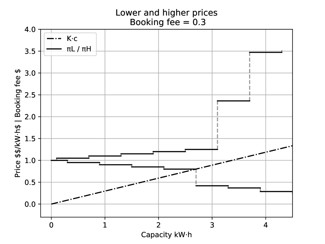
Figure 1: Example of TLOU pricing

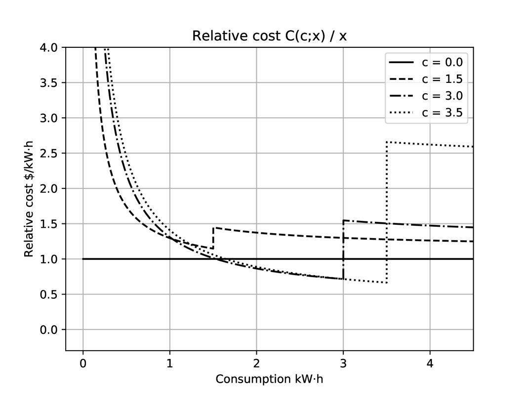
Figure 2: Relative cost of energy vs consumption for different capacities

The supplier first builds their set of options based on prior consumption data. In the proposed method, the prior discrete distribution used can be conditioned on some independent variables if they are known and influence the consumption (e.g. forecast external temperature or day of the week). They can then pick a pricing setting for a given day based on generation-side considerations and constraints, including the option to stay at a flat Time-of-Use tariff for some or all time frames.

Bilevel model of the supplier problem

The supplier wishes to determine an optimal set of pricing options at any capacity level. In the model developed in this section, we consider a discrete probability distribution with a finite support, derive some properties of the cost structure which we then leverage to formulate the optimization problem in a tractable form.

At any capacity level, the decision process of the supplier involves two objectives, the expected revenue from the tariff and the guarantee of an upper bound on the consumption. The expected revenue is given by:

$$\mathcal{C}(c)=K\cdot c+\sum_{\omega\in\Omega^{-}(c)}x_{\omega}p_{\omega}\pi^{L}(c)+\sum_{\omega\in\Omega^{+}(c)}x_{\omega}p_{\omega}\pi^{H}(c)$$ (4)

with any capacity booked defining a partition of the set of scenarios:

$$\Omega^{-}(c)=\{\omega\in\Omega,x_{\omega}\leq c\}$$ (5)

$$\Omega^{+}(c)=\{\omega\in\Omega,x_{\omega}>c\}$$ (6)

The function $\mathcal{C}(c)$ is minimized by the user with respect to their decision $c$. It is non-linear, non-smooth and discontinuous because of the partition of the scenarios by $c$ and the transition between steps of the pricing curves $\pi^{L}(c)$, $\pi^{H}(c)$. Both the user and supplier problems are thus intractable with this initial formulation. Proposition 3.1 shows that only a discrete finite subset of capacity values are candidates to optimality for the user.

Proposition 3.1.

The optimal booked capacity for a user at a time frame $t$ belongs to a discrete and finite set of capacities $S_{t}$, defined as:

$$\centering S_{t}=\{0\}\cup C^{L}\cup\Omega_{t}\@add@centering$$ (7)

with $\Omega$ the set of consumption scenarios.

Proof.

The user objective function is the sum of the booking cost and the expected electricity cost. The booking cost is linear in the booked capacity, with a positive slope equal to the booking fee. The expected electricity cost is piecewise constant in the booked capacity, with discontinuities at steps of both of the price curves because of the $\pi^{L}$ and $\pi^{H}$ prices and at possible load levels because of the transfer of a load from $\Omega^{+}$ to the $\Omega^{-}$ set. This can be highlighted using the indicator functions associated with each of the two sets:

$$\text{1}^{-}(\omega,c)=\begin{cases}1,&\mbox{if $x_{\omega}\leq c$,}\\ 0&\mbox{otherwise.}\end{cases}$$ (8)

$$\text{1}^{+}(\omega,c)=1-\text{1}^{-}(\omega,c)$$ (9)

The expression of the user expected cost becomes:

$$\mathcal{C}(c)=K\cdot c+\\ \sum_{\omega\in\Omega}x_{\omega}\cdot p_{\omega}\cdot\left(\pi^{L}(c)\cdot\text{1}^{-}(\omega,c)+\pi^{H}(c)\cdot\text{1}^{+}(\omega,c)\right)$$ (10)

The sum of the two terms is therefore piecewise linear with a positive slope. On any interval between the discontinuity points, the optimal value lies on the lower bound, which can be any point of $C^{L}$, $C^{H}$, $\Omega$ or 0.

Furthermore, let $\mathcal{C}(c)$ be the user cost for a booked capacity and $\bar{c}$ such that $\bar{c}\in C^{H}$ and $\bar{c}\notin\{0\}\cup C^{L}\cup\Omega$. The higher tariff levels are monotonically increasing. Let $\varepsilon>0$ be sufficiently small such that:

$$\pi^{H}(\bar{c}-\varepsilon) =\pi_{n},$$

$$\pi^{H}(\bar{c}+\varepsilon) =\pi_{n+1}>\pi_{n},$$

$$\pi^{L}(\bar{c}-\varepsilon) =\pi^{L}(\bar{c}+\varepsilon)=\pi^{L}_{m},$$

$$\nexists x_{\omega},\ \omega\in \Omega\text{ s.t. }\bar{c}-\varepsilon\leq x_{\omega}\leq\bar{c}+\varepsilon.$$

The last condition guarantees there is no load value in the $\left[\bar{c}-\varepsilon,\bar{c}+\varepsilon\right]$ interval and can also be expressed in terms of the two load sets split by the capacity:

$$\Omega^{+}(\bar{c}-\varepsilon)=\Omega^{+}(\bar{c}+\varepsilon)\ \text{and}\ \ \Omega^{-}(\bar{c}-\varepsilon)=\Omega^{-}(\bar{c}+\varepsilon).$$

Then if such $\varepsilon$ exists, we find that:

$$\mathcal{C}(\bar{c}-\varepsilon)=K\cdot(\bar{c}-\varepsilon)+\sum_{\omega\in\Omega^{-}(\bar{c})}\pi^{L}_{m}\cdot x_{\omega}+\sum_{x\in\Omega^{+}(\bar{c})}\pi^{H}_{n}\cdot x_{\omega},$$

$$\mathcal{C}(\bar{c}+\varepsilon)=K\cdot(\bar{c}+\varepsilon)+\sum_{\omega\in\Omega^{-}(\bar{c})}\pi^{L}_{m}\cdot x_{\omega}+\sum_{\omega\in\Omega^{+}(\bar{c})}\pi^{H}_{n+1}\cdot x_{\omega},$$

$$\mathcal{C}(\bar{c}+\varepsilon)-\mathcal{C}(\bar{c}-\varepsilon)=2\varepsilon K+\sum_{\omega\in\Omega^{+}(\bar{c})}(\pi^{H}_{n+1}-\pi^{H}_{n})\cdot x_{\omega},$$

$$\mathcal{C}(\bar{c}+\varepsilon)-\mathcal{C}(\bar{c}-\varepsilon)>0.$$

The discontinuity on any $x\in C^{H}$ is therefore always positive and cannot be a candidate for optimality. It follows that optimality candidates are restricted to the set $S=\{0\}\cup C^{L}\cup\Omega$. ∎

Proposition 3.1 means we can replace the continuous decision set of capacities with a discrete set that can be enumerated.

The guarantee of an upper bound on the consumption $\mathcal{G}$ corresponds to the incentive given to the user against consuming above the considered capacity. It is the second objective, given by the difference in cost at the capacity, which is the immediate difference in total cost at the transition from lower to higher tariff:

$$\mathcal{G}(c,\pi^{L},\pi^{H})=c_{t}\cdot\left(\pi^{H}(c)-\pi^{L}(c)\right).$$ (11)

The supplier needs to include the user behavior and optimal reaction in their decision-making process, which can be done by a bilevel constraint:

$$c_{t}\in arg\min_{c}\mathcal{C}(c).$$ (12)

The user thus books the least-cost option at each time frame, given the corresponding probability distribution. Given the finite set of optimal candidates $S_{t}$ defined in 3.1, this constraint can be re-written as:

$$\mathcal{C}(c_{t})\leq\mathcal{C}(c)\,\,\forall c\in S_{t}.$$ (13)

If multiple choices of $c$ yield the minimum cost, the choice of the user is not well-defined. The supplier would want to ensure the uniqueness of the preferred solution by making it lower than the expected cost of any other capacity candidate by a fixed quantity $\delta>0$. This quantity can be interpreted as the conservativeness of the user (unwillingness to move to an optimal solution up to a difference of $\delta$). It is a parameter of the decision-making process, estimated by the supplier. The lower-level optimality constraint is then for a preferred candidate $k$:

$$\mathcal{C}(c_{tk},K,\pi^{L},\pi^{H})\leq\mathcal{C}(c_{tl},K,\pi^{L},\pi^{H})-\delta\,\,\forall l\in S_{t}\backslash k.$$ (14)

Additional contractual constraints

In order to obtain regular price steps, the contract between supplier and consumer can include further constraints on the space of pricing parameters. We include three types of constraints: lower and upper bounds on the booking fee $K$, minimum and maximum increase at each step of the higher price and minimum and maximum decrease at each step of the higher price. All these can be expressed as linear constraints, and we gather them under the constraint set:

$$(K,\pi^{L},\pi^{H})\in\Phi.$$ (15)

Complete optimization model

The model is defined for each of the capacity candidates and is thus noted $\mathcal{P}_{tk}$ for candidate $k$ and time frame $t$:

$$\max_{K,\pi^{L},\pi^{H}} \left(\mathcal{C}(c_{tk},K,\pi^{L},\pi^{H}),\mathcal{G}(c_{tk},\pi^{L},\pi^{H})\right)$$ (16)

$$(K,\pi^{L},\pi^{H})\in\Phi$$ (17)

$$\mathcal{C}(c_{tk},K,\pi^{L},\pi^{H})\leq\mathcal{C}(c_{lt},K,\pi^{L},\pi^{H})-\delta\,\,\forall l\in S_{t}\backslash k,$$ (18)

where

$$\mathcal{C}(c_{tk},K,\pi^{L},\pi^{H}) =$$

$$K\cdot c_{tk} +\sum_{\omega\in\Omega^{-}_{t}(c_{tk})}x_{\omega}p{\omega}\pi^{L}_{k}+\sum_{\omega\in\Omega^{+}_{t}(c_{tk})}x_{\omega}p_{\omega}\pi^{H}_{k},$$ (19)

$$\mathcal{G}(c_{tk},\pi^{L},\pi^{H}) =c_{tk}\cdot\left(\pi^{H}(c)-\pi^{L}(c)\right).$$ (20)

Solution method and computational experiments

The proposed model was implemented and tested using historical consumption data[14] measured on a pilot house. The instantaneous consumption was measured every two minutes during 47 months on a residential building by the energy supplier and grid operator EDF[15]. Since the focus is the energy consumed within a given time frame, the instantaneous power can be averaged for each hour, yielding the energy in $kW\cdot h$ and avoiding issues of missing measurements in the dataset. Data preprocessing, density estimation and discretization, and visualization were performed using Julia [16], matplotlib [17] and KernelDensity.jl [18]. The construction and optimization of the model were carried out using CLP from the COIN-OR project [19] as a linear solver and JuMP [20]. For all experiments where it is not specified, an inertia of $\delta=0.05$ has been applied. For every time frame and for all capacity candidates, the bi-objective supplier problem with objectives $(\mathcal{C},\mathcal{G})$ is solved with the $\varepsilon$-constraint method implemented in MultiJuMP.jl[21]. In all cases, the objectives are found to be non-conflicting, in the sense that the utopia point of the multi-objective problem is feasible and reached. This implies that a lexicographic multi-objective optimization solves the problem and reaches the utopia point, but does not guarantee that this holds for all problem configurations.

Figure 4 shows the number of options computed at each hourly time frame and Figure 4 the capacity level in $kW\cdot h$ of each option. The option of a capacity level of 0 is always possible. Two examples of TLOU settings obtained are presented in Figures 6 and 6.

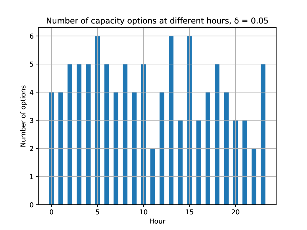
Figure 3: Number of options at different hours

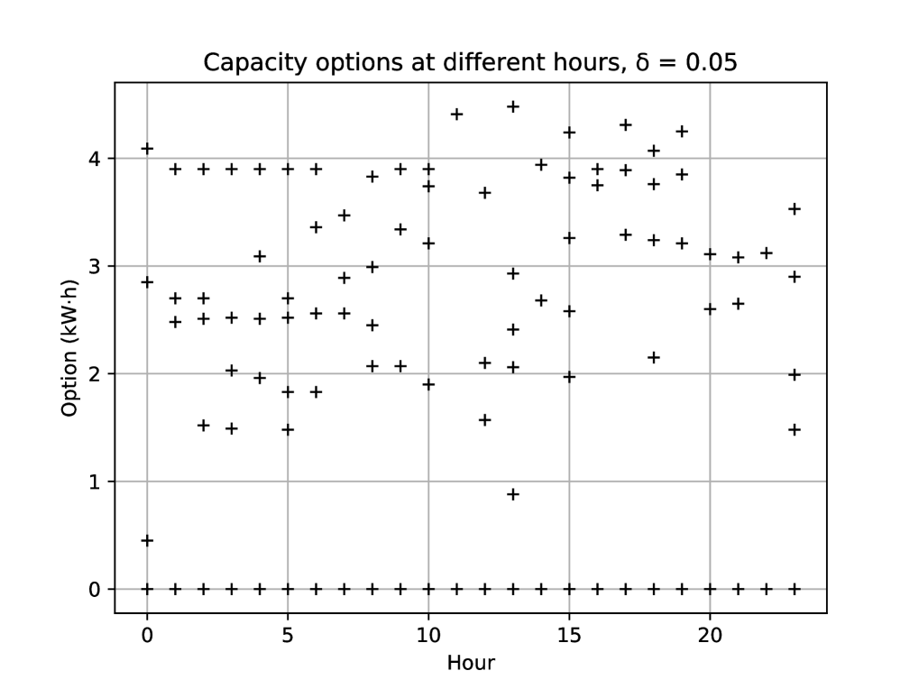
Figure 4: Capacity levels of options at different hours

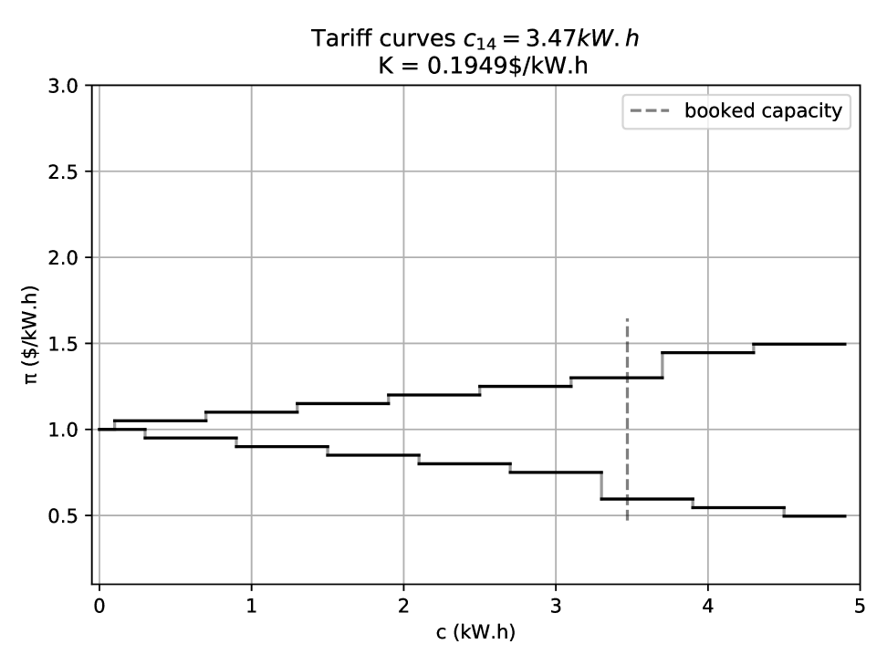
Figure 5: TLOU price settings to incentive for capacity $c=3.47kW\cdot h$

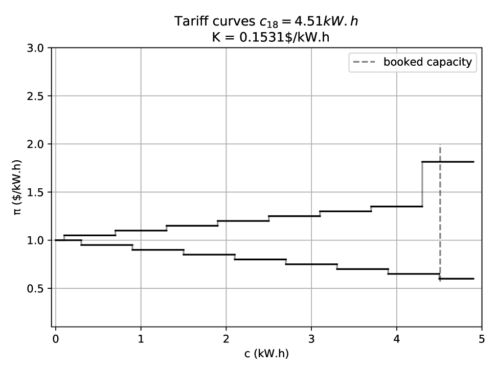
Figure 6: TLOU price settings to incentive for capacity $c=4.51kW\cdot h$

The expected cost for the user of booking any capacity, given the price setting provided in Figure 6 is shown Figure 7. The most notable result is that in all cases tested, the utopia point, defined as the optimal value of the two objectives optimized separately, is reachable. This result is conceivable given that the supplier decision is taken in a high-level space, allowing multiple solutions to be optimal with respect to the revenue. In order to ensure the guarantee-maximizing optimal solution, a two-step process lexicographic multi-optimization procedure is used:

1. Solve the revenue-maximizing problem to obtain the maximal reachable revenue $v$.

2. Solve the guarantee-maximizing problem, while constraining a revenue $\mathcal{C}(\cdot)\geq v$.

Figures 9 and 9 present a TLOU configuration optimized for costs only and for cost and guarantee.

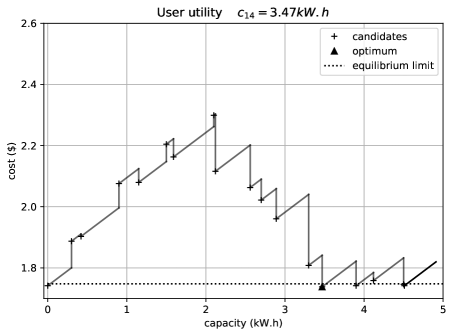
Figure 7: Expected cost for any capacity booked under the price settings of Figure 6

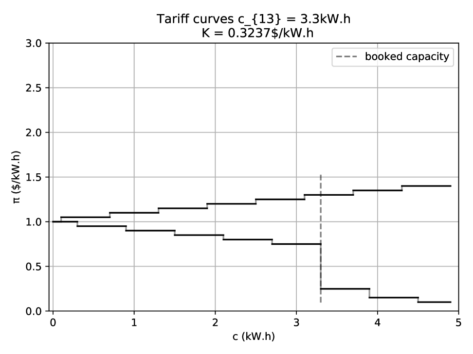
Figure 8: TLOU price settings for revenue maximization only

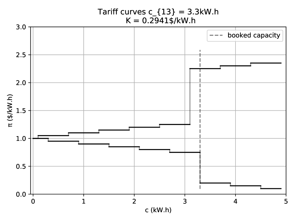
Figure 9: TLOU price settings after lexicographic optimization

All the models solved are linear optimization problems with a fixed number of variables and a number of constraints growing linearly with the number of scenarios considered. However, all these constraints are of type:

$$\mathcal{C}(c_{tk},K,\pi^{L},\pi^{H})\leq\mathcal{C}(c_{tl},K,\pi^{L},\pi^{H})-\delta\,\,\forall l\in S_{t}\backslash k.$$ (21)

This is equivalent to:

$$\mathcal{C}(c_{tk},K,\pi^{L},\pi^{H})\leq\min_{l\in S_{t}\backslash k}\mathcal{C}(c_{tl},K,\pi^{L},\pi^{H})-\delta.$$ (22)

Therefore, at most one of the $l$ will be active with a non-zero dual cost. The method can thus be scaled to a greater number of scenarios by adding these constraints on the fly.

With the current discretized distributions containing between 5 and 10 scenarios, the mean and median times to compute the whole solutions for all candidate capacities are below $\frac{1}{40}$ of a second. These metrics are obtained using the BenchmarkTools.jl package[22].

A study of the influence of the $\delta$ parameter is summarized Figure 10. For any hour, there always exists a maximum value $\delta_{max}$ above which it becomes impossible to make a solution better for the lower-level than the baseline with a difference greater than $\delta_{max}$.

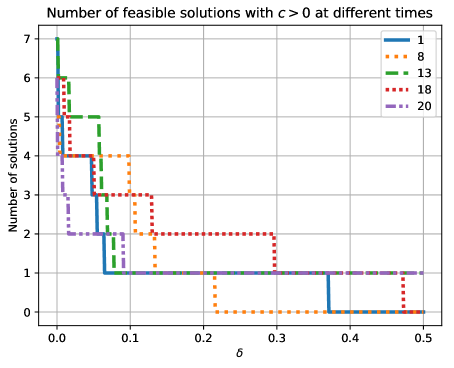
Figure 10: Number of non-zero capacity solutions

Conclusion

TLOU is designed to price energy across time and to reflect varying costs and requirements from the generation side. Defining two objectives for the supplier, we built the set of cost-optimal price settings maximizing the guarantee in a lexicographic fashion. Computations on distributions built from real data show the effectiveness of the method, requiring a low runtime to compute the set of solutions. Future research will consider continuous probability distributions of the consumption and the price-setting problem with multiple users.

References

- [1] Albadi, M. H. and El-Saadany, E. F. A summary of demand response in electricity markets. Electric Power Systems Research 78(11), 1989–1996 (2008).
- [2] US Federal Energy Regulatory Commission (FERC). Assessment of Demand Response and Advanced Metering, https://www.ferc.gov/legal/staff-reports/12-20-12-demand-response.pdf, 12 (2012).
- [3] Vuelvas, J., Ruiz, F., and Gruosso, G. Limiting gaming opportunities on incentive-based demand response programs. Applied Energy 225, 668 – 681 (2018).
- [4] Dempe, S., Kalashnikov, V., Prez-Valds, G. A., and Kalashnykova, N. Bilevel Programming Problems: Theory, Algorithms and Applications to Energy Networks. Springer Publishing Company, Incorporated, (2015).
- [5] Colson, B., Marcotte, P., and Savard, G. An overview of bilevel optimization. Annals of Operations Research 153(1), 235–256 (2007).
- [6] Shi, X. and Xia, H. S. Model and interactive algorithm of bi-level multi-objective decision-making with multiple interconnected decision makers. Journal of Multi-Criteria Decision Analysis 10(1), 27–34 (2001).
- [7] Fernández-Blanco, R., Arroyo, J. M., and Alguacil, N. On the Solution of Revenue- and Network-Constrained Day-Ahead Market Clearing Under Marginal Pricing Part I: An Exact Bilevel Programming Approach. IEEE Transactions on Power Systems 32(1), 208–219 jan (2017).
- [8] Fernández-Blanco, R., Arroyo, J. M., and Alguacil, N. On the Solution of Revenue- and Network-Constrained Day-Ahead Market Clearing Under Marginal Pricing Part II: Case Studies. IEEE Transactions on Power Systems 32(1), 220–227 jan (2017).
- [9] Street, A., Moreira, A., and Arroyo, J. M. Energy and reserve scheduling under a joint generation and transmission security criterion: An adjustable robust optimization approach. IEEE Transactions on Power Systems 29(1), 3–14 Jan (2014).
- [10] Bahrami, S., Amini, M. H., Shafie-khah, M., and Catalao, J. P. S. A Decentralized Renewable Generation Management and Demand Response in Power Distribution Networks. IEEE Transactions on Sustainable Energy 9(4), 1783–1797 (2018).
- [11] Yang, J., Zhao, J., Wen, F., and Dong, Z. Y. A framework of customizing electricity retail prices. IEEE Transactions on Power Systems 33(3), 2415–2428 May (2018).
- [12] Gomez-Herrera, J. A. and Anjos, M. F. Optimization-based estimation of power capacity profiles for activity-based residential loads. International Journal of Electrical Power & Energy Systems 104, 664–672 jan (2019).
- [13] Koliou, E., Eid, C., Chaves-Ávila, J. P., and Hakvoort, R. A. Demand response in liberalized electricity markets: Analysis of aggregated load participation in the german balancing mechanism. Energy 71, 245 – 254 (2014).
- [14] Dheeru, D. and Karra Taniskidou, E. UCI machine learning repository. http://archive.ics.uci.edu/ml, (2017).
- [15] Hébrail, G. and Bérard, A. Individual household electric power consumption data set. https://archive.ics.uci.edu/ml/datasets/individual+household+electric+power+consumption, 08 (2012).
- [16] Bezanson, J., Edelman, A., Karpinski, S., and Shah, V. Julia: A fresh approach to numerical computing. SIAM Review 59(1), 65–98 (2017).
- [17] Hunter, J. D. Matplotlib: A 2d graphics environment. Computing In Science & Engineering 9(3), 90–95 (2007).
- [18] JuliaStats. KernelDensity.jl v0.4.1. https://github.com/JuliaStats/KernelDensity.jl, 02 (2018).
- [19] Lougee-Heimer, R. The Common Optimization INterface for Operations Research: Promoting Open-source Software in the Operations Research Community. IBM J. Res. Dev. 47(1), 57–66 January (2003).
- [20] Dunning, I., Huchette, J., and Lubin, M. JuMP: A Modeling Language for Mathematical Optimization. SIAM Review 59(2), 295–320 (2017).
- [21] Riseth, A. N., Besançon, M., and Naiem, A. MultiJuMP.jl. https://doi.org/10.5281/zenodo.1042586, 02 (2019).
- [22] JuliaCI. BenchmarkTools.jl v0.3. https://github.com/JuliaCI/BenchmarkTools.jl, 05 (2018).