Transition from asynchronous to oscillatory dynamics in balanced spiking networks with instantaneous synapses

Abstract

We report a transition from asynchronous to oscillatory behaviour in balanced inhibitory networks for class I and II neurons with instantaneous synapses. Collective oscillations emerge for sufficiently connected networks. Their origin is understood in terms of a recently developed mean-field model, whose stable solution is a focus. Microscopic irregular firings, due to balance, trigger sustained oscillations by exciting the relaxation dynamics towards the macroscopic focus. The same mechanism induces in balanced excitatory-inhibitory networks quasi-periodic collective oscillations.

Introduction. Cortical neurons fire quite irregularly and with low firing rates, despite being subject to a continuous bombardment from thousands of pre-synaptic excitatory and inhibitory neurons Destexhe and Paré (1999). This apparent paradox can be solved by introducing the concept of balanced network, where excitation and inhibition balance each other and the neurons are kept near their firing threshold Vogels et al. (2005). In this regime spikes, representing the elementary units of information in the brain, are elicited by stochastic fluctuations in the net input current yielding an irregular microscopic activity, while neurons can promptly respond to input modifications Denève and Machens (2016).

In neural network models balance can emerge spontaneously in coupled excitatory and inhibitory populations thanks to the dynamical adjustment of their firing rates van Vreeswijk and Sompolinsky (1996); Brunel (2000); Renart et al. (2010); Litwin-Kumar and Doiron (2012); Kadmon and Sompolinsky (2015); Monteforte and Wolf (2010). The usually observed dynamics is an asynchronous state characterized by irregular neural firing joined to stationary firing rates van Vreeswijk and Sompolinsky (1996); Renart et al. (2010); Litwin-Kumar and Doiron (2012); Monteforte and Wolf (2010). The asynchronous state has been experimentally observed both in vivo and in vitro Barral and Reyes (2016); Dehghani et al. (2016), however this is not the only state observable during spontaneous cortical activity. In particular, during spontaneous cortical oscillations excitation and inhibition wax and wane together Okun and Lampl (2008), suggesting that balancing is crucial for the occurrence of these oscillations with inhibition representing the essential component for the emergence of the synchronous activity Isaacson and Scanziani (2011); Le Van Quyen et al. (2016).

The emergence of collective oscillations (COs) in inhibitory networks has been widely investigated in networks of spiking leaky integrate-and-fire (LIF) neurons. In particular, it has been demonstrated that COs emerge from asynchronous states via Hopf bifurcations in presence of an additional time scale, beyond the one associated to the membrane potential evolution, which can be the transmission delay Brunel and Hakim (1999); Brunel (2000) or a finite synaptic time Van Vreeswijk et al. (1994). As the frequency of the COs is related to such external time scale this mechanism is normally related to fast ($>$30 Hz) oscillations. Nevertheless, despite many theoretical studies, it remains unclear which other mechanisms could be invoked to justify the broad range of COs’ frequencies observed experimentally Chen et al. (2017).

In this Letter we present a novel mechanism for the emergence of COs in balanced spiking inhibitory networks in absence of any synaptic or delay time scale. In particular, we show for class I and II neurons Izhikevich (2007) that COs arise from an asynchronous state by increasing the network connectivity (in-degree). Furthermore, we show that the COs can survive only in presence of irregular spiking dynamics due to the dynamical balance. The origin of COs can be explained by considering the phenomenon at a macroscopic level, in particular we extend an exact mean-field formulation for the spiking dynamics of Quadratic Integrate-and-Fire (QIF) neurons Montbrió et al. (2015) to sparse balanced networks. An analytic stability analysis of the mean-field model reveals that the asymptotic solution for the macroscopic model is a stable focus and determines the frequency of the associated relaxation oscillations. The agreement of this relaxation frequency with the COs’ one measured in the spiking network suggests that the irregular microscopic firings of the neurons are responsible for the emergence of sustained COs corresponding to the relaxation dynamics towards the macroscopic focus. This mechanism elicits COs through the excitation of an internal macroscopic time scale, that can range from seconds to tens of milliseconds, yielding a broad range of collective oscillatory frequencies. We then analyse balanced excitatory-inhibitory populations revealing the existence of COs characterized by two distinct frequencies, whose emergence is due, also in this case, to the excitation of a mean-field focus induced by fluctuation-driven microscopic dynamics.

The model. We consider a balanced network of $N$ pulse-coupled inhibitory neurons, whose membrane potential evolves as

$$\tau_{m}\dot{v}_{i}=F(v_{i})+I-2\tau_{m}g\sum_{j\in pre(i)}\varepsilon_{ij}\delta(t-t_{j})$$ (1)

where $I$ is the external DC current, $g$ is the inhibitory synaptic coupling, $\tau_{m}=20$ ms is the membrane time constant and fast synapses (idealized as $\delta$-pulses) are considered. The neurons are randomly connected, with in-degrees $k_{i}$ distributed according to a Lorentzian PDF peaked at $K$ and with a half-width half-maximum (HWHM) $\Delta_{K}$. The elements of the corresponding adjacency matrix $\varepsilon_{ij}$ are one (zero) if the neuron $j$ is connected (or not) to neuron $i$. We consider two paradigmatic models of spiking neuron: the quadratic-integrate and fire (QIF) with $F(v)=v^{2}$ Ermentrout and Kopell (1986), which is a current-based model of class I excitability; and the Morris-Lecar (ML) Morris and Lecar (1981); mod representing a conductance-based class II excitable membrane. The DC current and the coupling are rescaled with the median in-degree as $I=\sqrt{K}I_{0}$ and $g=g_{0}/\sqrt{K}$, as usually done in order to achieve a self-sustained balanced state for sufficiently large in-degrees van Vreeswijk and Sompolinsky (1996); Renart et al. (2010); Litwin-Kumar and Doiron (2012); Kadmon and Sompolinsky (2015); Jahnke et al. (2009); Monteforte and Wolf (2010, 2012). Furthermore, in analogy with Erdös-Renyi networks we assume $\Delta_{K}=\Delta_{0}\sqrt{K}$. We have verified that the reported phenomena are not related to the peculiar choice of the distribution of the in-degrees, namely Lorentzian, needed to obtain an exact mean-field formulation for the network evolution Montbrió et al. (2015), but that they can be observed also for more standard distributions, like Erdös-Renyi and Gaussian ones (for more details see the SM mod and Bi et al. ).

In order to characterize the network dynamics we measure the mean membrane potential ${V}(t)=\sum_{i=1}^{N}v_{i}(t)/N$, the instantaneous firing rate $R(t)$, corresponding to the number of spikes emitted per unit of time, as well as the population averaged coefficient of variation ${CV}$ CV measuring the fluctuations in the neuron dynamics. Furthermore, the level of coherence in the neural activity can be quantified in terms of the following indicator Golomb (2007)

$$\rho\equiv\left(\frac{\sigma_{V}^{2}}{\sum_{i=1}^{N}\sigma^{2}_{i}/N}\right)^{1/2}\;,$$ (2)

where $\sigma_{V}$ is the standard deviation of the mean membrane potential, $\sigma^{2}_{i}={\langle V_{i}^{2}\rangle}-{\langle V_{i}\rangle}^{2}$ and $\langle\cdot\rangle$ denotes a time average. A coherent macroscopic activity is associated to a finite value of $\rho$ (perfect synchrony corresponds to $\rho=1$), while an asynchronous dynamics to a vanishingly small $\rho\approx{\cal O}(1/\sqrt{N})$. Time averages and fluctuations are usually estimated on time intervals $\simeq 120$ s, after discarding transients $\simeq 2$ s.

Results. In both models we can observe collective firings, or population bursts, occurring at almost constant frequency $\nu_{osc}$. As shown in Fig. 1, despite the almost regular macroscopic oscillations in the firing rate $R(t)$ and in the mean membrane potential $V(t)$, the microscopic dynamics of the neurons $v_{i}(t)$ is definitely irregular. The latter behaviour is expected for balanced networks, where the dynamics of the neurons driven by the fluctuations in the input current, however usually the collective dynamics is asynchronous and not characterized by COs as in the present case van Vreeswijk and Sompolinsky (1996); Renart et al. (2010); Litwin-Kumar and Doiron (2012); Kadmon and Sompolinsky (2015); Jahnke et al. (2009); Monteforte and Wolf (2010, 2012).

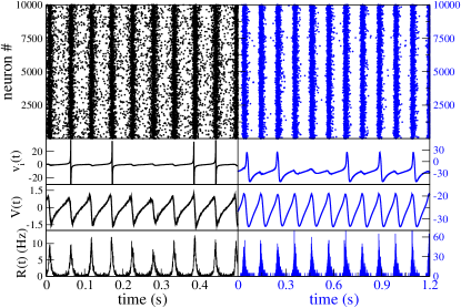
Figure 1: The panels show (from top to bottom) the raster plots and the corresponding time traces for the membrane potential $v_{i}(t)$ of a representative neuron, for ${V}(t)$ and $R(t)$. Left row (black): QIF and right row (blue): ML. The parameter values are $N=10000$, $K=1000$, $\Delta=0.3$, $g_{0}=1$ and $I_{0}=0.015$.

Asynchronous dynamics is indeed observable also for our models for sufficiently sparse networks (small $K$), indeed a clear transition is observable from an asynchronous state to collective oscillations for $K$ larger than a critical value $K_{c}$. As observable from Figs. 2 (a,b), where we report the coherence indicator $\rho$ as a function of $K$ for various system sizes from $N=2,000$ to $N=20,000$. In particular, $\rho$ vanishes as $N^{-1/2}$ for $K<K_{c}$ (as we have verified), while it stays finite above the transition thus indicating the presence of collective motion. This transition resembles those reported for sparse LIF networks with finite synaptic time scales in Golomb and Hansel (2000); Luccioli et al. (2012) or with finite time delay in Brunel and Hakim (1999); Brunel (2000). However, Poissonian-like dynamics of the single neurons has been reported only in Brunel and Hakim (1999); Brunel (2000).

In the present case, in both the observed dynamical regimes the microscopic dynamics remains quite irregular for all the considered $K$ and system size $N$, as testified by the fact that ${CV}\simeq 0.8$ for the QIF and ${CV}\geq 1$ for the ML (as shown in the insets of Fig. 2 (a,b)). The relevance of the microscopic fluctuations for the existence of the collective oscillations in this system can be appreciated by considering the behaviour of $\rho$ and $CV$ as a function of the external current $I_{0}$ and of the parameter controlling the structural heterogeneity, namely $\Delta_{0}$. The results of these analysis are shown in Figs. 2 (c) and (d) for the QIF and for $N=2,000$, 10,000 and 20,000. In both cases we fixed a in-degree $K>K_{c}$ in order to observe collective oscillations and then we increased $I_{0}$ or $\Delta_{0}$. In both cases we observe that for large $I_{0}$ ($\Delta_{0}$) the microscopic dynamics is now imbalanced with few neurons firing regularly with high rates and the majority of neurons suppressed by this high activity. This induces a vanishing of the $CV$, which somehow measures the degree of irregularity in the microscopic dynamics. At large $I_{0}$ the dynamics of the network is controlled by neurons definitely supra-threshold and the dynamics becomes mean-driven Renart et al. (2007); Angulo-Garcia et al. (2017). The same occurs by increasing $\Delta_{0}$, when the heterogeneity in the in-degree distribution becomes sufficiently large only few neurons, the ones with in-degrees in proximity of the mean $K$, can balance their activity, while for the remaining neurons it is no more possible to satisfy the balance conditions, as recently shown in Landau et al. (2016); Pyle and Rosenbaum (2016); Farkhooi and Stannat (2017). As a result, COs disappear as soon as the microscopic fluctuations, due to the balanced irregular spiking activity, vanish.

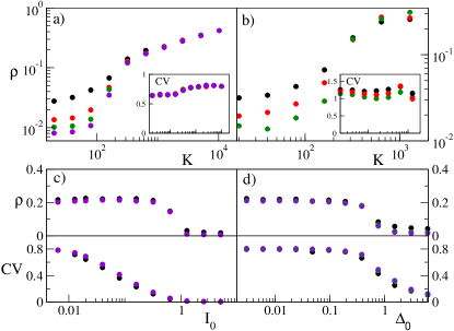
Figure 2: Upper panels: order parameter $\rho$ versus $K$ for QIF (a) and ML (b), the inset report the corresponding CVs. The lower panels display in the upper part $\rho$ and in the lower one the $CV$ versus $I_{0}$ (c) and $\Delta_{0}$ (d) for the QIF. The data refer to various system sizes: namely $N=2000$ (black), 5000 (red), 10,000 (green) and 20,000 (violet). The employed parameters are $I_{0}=0.1$, $g_{0}=5$, and $\Delta_{0}=1$ for ML (b); for QIF $g_{0}=1$, $\Delta_{0}=0.1$, $I_{0}=0.006$, $K=1000$.

Effective Mean-Field Model. In order to understand the origin of these macroscopic oscillations we consider an exact macroscopic model recently derived in Montbrió et al. (2015) for fully coupled networks of pulse-coupled QIF with synaptic couplings randomly distributed according to a Lorentzian. The mean-field dynamics of this QIF network can be expressed in terms of only two collective variables (namely, $V$ and $R$), as follows  Montbrió et al. (2015):

$$\dot{R}=\frac{R}{\tau_{m}}\left(2V+\frac{\Gamma}{\pi}\right)\enskip,\enskip\dot{V}=\frac{V^{2}+I}{\tau_{m}}+R{\bar{g}}-(\pi R)^{2}\tau_{m}$$ (3)

where ${\bar{g}}$ is the median and $\Gamma$ the HWHM of the Lorentzian distribution of the synaptic couplings.

Such formulation can be applied to the sparse network studied in this Letter, indeed the quenched disorder in the connectivity can be rephrased in terms of a random synaptic coupling di Volo et al. (2014). Namely, each neuron $i$ is subject to an average inhibitory synaptic current of amplitude $g_{0}k_{i}R/(\sqrt{K})$ proportional to its in-degree $k_{i}$. Therefore we can consider the neurons as fully coupled, but with random values of the coupling distributed as a Lorentzian of median ${\bar{g}}=-g_{0}\sqrt{K}$ and HWHM $\Gamma=g_{0}\Delta_{0}$. The mean-field formulation (3) takes now the expression:

$$\tau_{m}\dot{R}=R(2V+\frac{g_{0}\Delta_{0}}{\pi})$$ (4)

$$\tau_{m}\dot{V}=V^{2}+\sqrt{K}(I_{0}-\tau_{m}g_{0}R)-(\pi R\tau_{m})^{2}\enskip.$$ (5)

As we will verify in the following, this formulation represents a quite good approximation of the collective dynamics of our network. Therefore we can safely employ such effective mean-field model to interpret the observed phenomena and to obtain theoretical predictions for the spiking network.

Let us first consider the fixed point solutions $({\bar{V}},{\bar{R}})$ of Eqs. (4,5). The result for the average membrane potential is ${\bar{V}}=(-g_{0}\Delta_{0})/(2\pi)$, while the firing rate is given by the following expression

$${\bar{R}}\tau_{m}=\frac{g_{0}\sqrt{K}}{2\pi^{2}}\left(\sqrt{1+\frac{4\pi^{2}}{\sqrt{K}}\frac{I_{0}}{g_{0}^{2}}+\frac{\Delta_{0}^{2}}{K}}-1\right)\enskip.$$ (6)

This theoretical result reproduces quite well with the simulation findings for the QIF spiking network in the asynchronous regime (observable for sufficiently high $\Delta_{0}$ and $I_{0}$) over a quite broad range of connectivities (namely, $10\leq K\leq 10^{4}$), as shown in Fig.3 (a). At the leading order in $K$, the firing rate (6) is given by $R_{a}\tau_{m}=I_{0}/g_{0}$, which represents the asymptotic result to which the balanced inhibitory dynamics converges for sufficiently large in-degrees irrespectively of the considered neuronal model, as shown in Fig.3 (a) and (b) for the QIF and ML models and as previously reported in Monteforte and Wolf (2012) for Leaky Integrate-and-Fire (LIF) neurons. In particular, for the ML model the asymptotic result $R_{a}$ is attained already for $K\geq 500$, while for the QIF model in-degrees larger than $10^{4}$ are required.

The linear stability analysis of the solution $({\bar{V}},{\bar{R}})$ reveals that this is always a stable focus, characterized by two complex conjugates eigenvalues with a negative real part $\Lambda_{R}\tau_{m}=-\Delta_{0}/2\pi$ and an imaginary part $\Lambda_{I}\tau_{m}=\sqrt{2{\bar{R}}\tau_{m}(2\pi^{2}{\bar{R}}\tau_{m}+\sqrt{K}g_{0})-(\Delta_{0}/2\pi)^{2}}$. The frequency of the relaxation oscillations towards the stable fixed point solution is given by $\nu_{th}=\Lambda_{I}/2\pi$. This represents a good approximation of the frequency $\nu_{osc}$ of the sustained collective oscillations observed in the QIF network over a wide range of values ranging from ultra-slow rhythms to high $\gamma$ band oscillations, as shown in Fig. 3 (c). Furthermore, it can be shown that $\nu_{th}$ predicts the correcting scaling of $\nu_{osc}$ for the QIF for sufficiently large DC currents and/or median in-degree $K$, namely $\nu_{th}\approx I_{0}^{1/2}K^{1/4}$ (as shown in Fig. 3 (c) and (d)). For the ML we observe similar scaling behaviours for $\nu_{osc}$, with slightly different exponent, namely $\nu_{osc}\approx I_{0}^{0.4}$ and $\nu_{osc}\simeq K^{0.10}$, however in this case we have not a theoretical prediction to compare with (see the insets of Fig. 3 (c) and (d)).

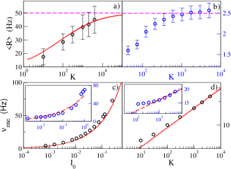
Figure 3: Upper panels: average firing rates $\langle R\rangle$ versus $K$ for QIF (a) and ML(b), the horizontal dashed (magenta) lines denote $R_{a}$ and the solid (red) line in (a) ${\bar{R}}$ in Eq. (6). The choice of parameters ($I_{0},\Delta_{0}$) sets the dynamics as asynchronous: $(1,3)$ in (a) and $(0.05,8)$ in (b). Lower panels: $\nu_{osc}$ versus $I_{0}$ (c) and versus $K$ (d) for the QIF, the insets display the same quantities for the ML. The red solid line in (c) refers to $\nu_{th}$, and in (d) to the theoretically predicted scaling $\nu_{th}\sim K^{\frac{1}{4}}$; the red dashed line in the inset of (c) and (d) to power-law fitting $\nu_{osc}\simeq I^{0.40}$ and $\nu_{osc}\simeq K^{0.10}$, respectively. Oscillatory dynamics is observable for the selected parameter’s values ($I_{0},\Delta_{0}$): $(0.05,0.3)$ in (c) and $(0.05,0.5)$ in (d). Other parameters’ values $N=10,000$, $g_{0}=1$, and $K=1000$ in (c).

Excitatory-inhibitory balanced populations So far we have considered only balanced inhibitory networks, but in the cortex the balance occurs among excitatory and inhibitory populations. To verify if also in this case collective oscillations could be identified we have considered a neural network composed of $80\%$ excitatory QIF neurons and $20\%$ inhibitory ones (for more details on the considered model see the SM in mod ). The analysis reveals that also in this case collective oscillations can be observed in the balanced network in presence of irregular microscopic dynamics of the neurons. This is evident from the raster plot reported in Fig. 4 (a). An important novelty is that now the oscillations are characterized by two fundamental frequencies as it becomes evident from the analysis of the power spectrum $S(\nu)$ of the mean voltage $V(t)$ shown in Fig. 4 (b). As expected for a noisy quasi-periodic dynamics, the spectrum reveals peaks of finite width at frequencies that can be obtained as linear combinations of two fundamental frequencies $\nu_{1}$ and $\nu_{2}$. The origin of the noisy contribution can be ascribed to the microscopic irregular firings of the neurons. Analogously to the inhibitory case, a theoretical prediction for the collective oscillation frequencies can be obtained by considering an effective mean-field model for the excitatory and inhibitory populations of QIF neurons. The model is now characterized by 4 variables, i.e. the mean membrane potential and the firing rate for each population, and also in this case one can find as stationary solutions of the model a stable focus. However, the stability of the focus is now controlled by two couples of complex conjugate eigenvalues, thus the relaxation dynamics of the mean-field towards the fixed point is quasi-periodic (see the SM for more details mod ). A comparison between the theoretical values of these relaxation frequencies and the measured oscillation frequencies $\nu_{1}$ and $\nu_{2}$ associated to the spiking network dynamics is reported in Figs. 4 (c) and (d) for a wide range of DC currents, revealing an overall good agreement. Thus suggesting that the mechanism responsible for the collective oscillations remains the same identified for the inhibitory network.

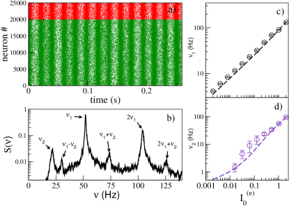
Figure 4: The raster plot for a network of $N_{E}=20,000$ excitatory (green) and $N_{I}=5,000$ inhibitory (red) QIF neurons is displayed in (a). In (c) and (d) the COs’ frequencies, measured from the power spectrum $S(\nu)$ of the mean voltage $V(t)$ (shown in (b)), are reported as symbols versus the excitatory DC current $I_{0}^{e}$. The dashed lines are the theoretical mean-field predictions. The values of the parameters are reported in mod .

Conclusions. We have shown that in balanced spiking networks with instantaneous synapses COs can be triggered by microscopic irregular fluctuations, whenever the neurons will share a sufficient number of common inputs. Therefore, for a sufficiently large in-degree the erratic spiking emissions can promote coherent dynamics. We have verified that the inclusion of a small synaptic time scale does not alter the overall scenario Bi et al. .

It is known that heuristic firing-rate models, characterized by a single scalar variable (e.g. the Wilson-Cowan model Wilson and Cowan (1972)), are unable to reproduce synchronization phenomena observed in spiking networks Schaffer et al. (2013); Devalle et al. (2017). In this Letter, we confirm that the inclusion of the membrane dynamics in the mean-field formulation is essential to correctly predict the frequencies of the COs, not only for finite synaptic times (as shown in Devalle et al. (2017)), but also for instantaneous synapses in dynamically balanced sparse networks. In this latter case, the internal time scale of the mean-field model controls the COs’ frequencies over a wide and continuous range. As we have verified, sustained oscillations can be triggered in the mean-field model by adding noise to the membrane dynamics. Therefore, an improvement of the mean-field theory here presented should include fluctuations around the mean values. A possible strategy could follow the approach reported in Schaffer et al. (2013) to derive high dimensional firing-rate models from the associated Fokker-Planck description of the neural dynamics Brunel and Hakim (1999); Brunel (2000). Of particular interest would be to understand if a two dimensional rate equation Schaffer et al. (2013) is sufficient to faithfully reproduce collective phenomena also in balanced networks.

Our results pave the way for a possible extension of the reported mean-field model to spatially extended balanced networks Kriener et al. (2013); Rosenbaum and Doiron (2014); Pyle and Rosenbaum (2017); Senk et al. (2018) by following the approach employed to develop neural fields from neural mass models Coombes (2006).