IPMU-18-0143

Do We Live in the Swampland?
Hitoshi Murayama^1,2,3, Masahito Yamazaki¹ and Tsutomu T. Yanagida^1
1Kavli Institute for the Physics and Mathematics of the Universe (WPI), University of Tokyo, Kashiwa, Chiba 277-8583, Japan ²Berkeley Center for Theoretical Physics and Department of Physics,University of California, Berkeley, CA 94720, USA ³Physics Division, Lawrence Berkeley National Laboratory, Berkeley, CA 94720, USA

A low-energy effective theory is said to be in the swampland if it does not have any consistent UV completion inside a theory of quantum gravity. The natural question is if the standard model of particle physics, possibly with some minimal extensions, are in the swampland or not. We discuss this question in view of the recent swampland conjectures. We prove a no-go theorem concerning the modification of the Higgs sector. Moreover, we find that QCD axion is incompatible with the recent swampland conjectures, unless some sophisticated possibilities are considered. We discuss the implications of this result for spontaneous breaking of CP symmetry. We comment on dynamical supersymmetry breaking as well as the issue of multi-valuedness of the potential.

1 Introduction

String theory has been one of the most promising candidates for the theory of quantum gravity. While string theory has been very successful in a number of different directions, a fundamental question is if it has any direct experimental consequences in particle phenomenology. The effective field theory dogma suggests that quantum gravity at the Planck scale is irrelevant for a particle physicist, who often studies energy scales much lower than the Planck scale.

However, there is growing evidence that a vast class of effective field theories, which are totally consistent as low-energy effective theories, do not have consistent UV completions with gravity included. In such cases, in the terminology of [1, 2], the low-energy effective theories are in the swampland as opposed to the landscape. Indeed, there are indications that a significant portion of the low-energy effective field theories fall into the swampland. If this is indeed the case, it could be misleading to be confined to the effective field theory framework: the constraints for the existence of suitable UV completion with gravity imposes important constraints for particle physics, which are hard to see otherwise.

It is then natural to ask the following question: is the standard model of particle physics, possibly with some extensions, be in the swampland or not? In this paper we discuss this question. Our main focus will be the QCD axion, which has long considered to be one of the most promising solutions to the strong CP problem [3, 4, 5, 6].

To set the stage, we begin by summarizing the recent swampland conjecture of [7]. We then recall the quintessence explanation for the present-day vacuum energy [7, 8] (section 3), and for the Higgs potential [9] (section 4). We then come to our main ingredient, the QCD axion. After pointing out the problem with QCD axion (section 5), we discuss some possible loop holes (section 6). Our conclusion is that the QCD axion is excluded by a set of swampland conjectures [7, 2, 10], unless exotic scenarios are considered. We discuss the implications of this result for the strong CP problem (section 7). We comment on dynamical supersymmetry breaking and multi-valuedness of the potential (section 8). We finally comment on the modification of the swampland conjecture (section 9) The Appendix (Appendix A) contains some no-go result for the modification of the Higgs potential. The mathematical result there could be useful for an analysis of the conjecture in [7] in other contexts.

2 Swampland Conjectures

Suppose that we have an effective field theory coupled with Einstein gravity, containing a finite number of scalar fields $\{\phi^{i}\}$. We then have the Lagrangian

$$\begin{split}\mathcal{L}=\sqrt{-g}\left[R+\sum_{i}D^{\mu}\phi^{i}D_{\mu}\phi^{i}+V_{\rm total}(\{\phi_{i}\})+\dots\right]\;.\end{split}$$ (1)

Here $V_{\rm total}(\{\phi_{i}\})$ is the potential for the scalar fields, and we added an index ‘total’ to emphasize that this is the full potential for all the scalar fields in the theory. Note that for the scalar fields we have chosen a canonical kinetic term in the Einstein frame. If this is not the case then a suitable re-parametrization of the fields is needed to bring the Lagrangian into the form of (1).

The question is when this theory has a well-defined UV completion inside a suitable theory of quantum gravity, such as string theory. In other words, is the theory in the swampland, or in the landscape?

In the literature several necessary conditions, for the effective theory to be in the landscape, have been proposed. We call these the swampland conjectures. Over the years several such conjectures have been proposed [1, 2, 10, 11, 7], see [12] for recent summary.

One of the most recent of such swampland conjectures is the following remarkable conjecture due to Obied et. al. [7]:

Conjecture 1 (de Sitter derivative conjecture): The potential $V_{\rm total}$ satisfies the following inequality:

$$\begin{split}M_{\rm Pl}\,||\nabla V_{\rm total}||>c_{\star}V_{\rm total}\;,\end{split}$$ (3)

where $c_{\star}$ is a $O(1)$ constant and $M_{\rm Pl}=2.4\times 10^{18}\textrm{ GeV}$ is the reduced Planck scale.

The precise optimal value of the $O(1)$ constant $c_{\star}$ depends on the setup. For example, four-dimensional compactifications of the eleven-dimensional supergravity suggests the value $c_{\star}=6/\sqrt{14}\sim 1.6$ [7]. Our discussion below, however, does not depend on the precise values of $c_{\star}$, and could easily accommodate the value $c_{\star}\sim 10^{-3}$, for example.

We will discuss the phenomenological consequences of this and other swampland conjectures. Note that even if the Conjecture 1 in itself does not hold in full generality, our conclusion still applies to some well-understood corners of string/M-theory vacua, as shown in the analysis of [13, 14, 7]. This is one of the reasons why the Conjecture 1 should be taken seriously.

3 Quintessence

An immediate consequence of the conjecture (3) is that there is no de Sitter vacua, even metastable ones [15, 7] (cf. [16, 17, 18]):

$$\begin{split}\quad V_{\rm total}>0\;,\quad\nabla V_{\rm total}=0\quad\textrm{not allowed}\;.\end{split}$$ (4)

This in particular excludes the constant positive cosmological constant. We can instead consider a dynamical vacuum energy as generated by a scalar field $Q$, the so-called quintessence field ([19, 20, 21], see [22] for review). This is an extremely light scalar field, and we can for example choose the potential to be

$$\begin{split}V_{Q}(Q)=\Lambda_{Q}^{4}\,e^{-c_{Q}\frac{Q}{M_{\rm Pl}}}\;,\end{split}$$ (5)

where $c_{Q}$ is some $O(1)$ constant. It was shown that this kind of potential can indeed be incorporated in supergravity, namely the effective field theory of string theory [23].

In this potential the shift of the origin of the quintessence field can be absorbed in the redefinition of the scale $\Lambda_{Q}^{4}$. We choose the present-day value of the quintessence field to be $Q/M_{\rm Pl}\sim 0$. To explain the current value of the cosmological constant, the energy scale $\Lambda_{Q}$ is chosen to be $\Lambda_{Q}\sim O(1)\textrm{ meV}$. The quintessence is the only scalar field at this energy scale, and the condition (3) is satisfied easily if $c_{Q}\geq c_{\star}$.

4 Higgs

In the minimal version of the standard model, the only fundamental scalar field is the Higgs particle. At the electroweak (EW) scale $\Lambda_{\rm EW}\sim O(100)\textrm{ GeV}$, the only scalar fields in the theory are the Higgs field $H$ and the quintessence field $Q$ introduced above.

The potential for the Higgs field is

$$\begin{split}V_{H}=\lambda(H^{2}-v^{2})^{2}\;,\end{split}$$ (6)

where $H$ is the absolute value of the complex Higgs field: in the following we always have the symmetry of rotating the phase of the complex Higgs field, and the phase part of the Higgs field will not play any role. The total potential at the EW scale is then

$$\begin{split}V_{\rm total}(Q,H)=V_{Q}(Q)+V_{H}(H)\;.\end{split}$$ (7)

The Higgs potential (6) has (a) a local minimum at $H^{2}=v^{2}$ and (b) a local maximum at $H=0$.

As already pointed out in [9], the latter (namely the local maximum (b)) is contradictory with the swampland conjecture (3). In the neighborhood of the point (b) we obtain $\partial_{H}V_{\rm total}(Q,H)=\partial_{H}V_{H}(H)\sim 0$, and hence $||\nabla V_{\rm total}(Q,H)||=\partial_{Q}V_{Q}(Q)\sim O(\Lambda_{Q}^{4})$. By contrast the value of the potential is given by $V_{\rm total}(Q,H)\sim O(\Lambda_{\rm EW}^{4})$ and is positive $V_{\rm total}(Q,H)>0$. We therefore obtain

$$\begin{split}0<M_{\rm Pl}\frac{||\nabla V_{\rm total}(Q,H)||}{V_{\rm total}(Q,H)}\sim O\left(\frac{\Lambda_{Q}^{4}}{\Lambda_{\rm EW}^{4}}\right)\sim O(10^{-56})\;,\end{split}$$ (8)

which is in sharp contradiction with the Conjecture 1 (3). Note that in this analysis we did not assume anything about the history of the Universe—the swampland conjecture applies to any possible field values which can be theoretically considered in the effective field theory.

One possibility to escape this contradiction is to modify the EW sector, and consider a coupling of the Higgs field to some other field. For example, we can introduce a real scalar field $S$ so that the potential is now given by

$$\begin{split}V_{H,S}=\lambda(H^{2}-v^{2})^{2}+\kappa(S-u)(H^{2}-w^{2})+\frac{m}{2}S^{2}+\Lambda_{S}^{4}\;,\end{split}$$ (9)

where we have introduced new dimension-full parameters $u,w,\kappa,m,\Lambda_{S}$, which are assumed to be in the electroweak scale. The potential (9) is the most general expression in $H^{2}$ and $S$ up to the quadratic order, up to a shift of the origin of $S$ and $H^{2}$. Since we have many free parameters, one might hope that one can adjust the free parameters such that there is no extremal values with positive potential values, perhaps at the cost of fine-tuning the parameters.

It turns out, however, this modification does not work—one either finds a de Sitter extremum of the potential and thus violating the conjecture (3), or the EW vacua becomes unstable (the determinant of the Hessian about the EW vacua becomes negative). The detailed analysis for this is provided in Appendix A. Indeed, we can show that this conclusion holds for a much broader class of models than the particular model (9) (see a no-go theorem in Appendix A). While we did not completely exclude the possible EW modifications, we believe that this is a strong evidence that the EW modification of the Higgs sector requires more sophisticated scenarios, to say the least.

Instead of modifying the EW sector, we can take advantage of the quintessence field, as already pointed out in [9]. Namely we can modify the Higgs potential to be

$$\begin{split}V^{\prime}_{H}(H)=e^{-c_{H}\frac{Q}{M_{\rm Pl}}}\lambda^{\prime}(H^{2}-v^{2})^{2}\;.\end{split}$$ (10)

We can then easily verify that the combined potential $V_{\rm total}(H,Q)=V_{Q}(Q)+V^{\prime}_{H}(H)$ does not have any extremal values. We therefore no longer have any contradiction with the Conjecture 1 in (3).

In conclusion, by applying the Conjecture 1 to the Higgs potential we obtained some supporting evidence for an existence of the quintessence field. This is independent from the argument from the previous section concerning the cosmological constant.

5 QCD Axion

In addition to the Higgs field, some extensions of the standard model could contain other scalar fields, at energy scales lower than the EW scale.

A good example is the QCD axion, which if present we will encounter at the QCD scale $\Lambda_{\rm QCD}\sim O(100)\textrm{ MeV}$. Since axions are abundant in string theory compactifications [25, 26], it might be natural to imagine that we have the QCD axion in the string/M theory landscape.

The QCD axion, which we denote by $a$, couples to the QCD gauge field as a dynamical $\theta$-angle:

$$\begin{split}\mathcal{L}_{\rm axion}=\frac{1}{32\pi^{2}}\frac{a}{f_{a}}e^{\mu\nu\rho\sigma}\textrm{Tr}F_{\mu\nu}F_{\rho\sigma},\end{split}$$ (11)

where $f_{a}$ is the axion decay constant.

Perturbatively we have a shift symmetry for the axion $a\to a+(\textrm{const.})$, which is broken only by the non-perturbative effects:

$$\begin{split}V_{\rm axion}(a)=\Lambda_{\rm QCD}^{4}\left[1-\cos\left(\frac{a}{f_{a}}\right)\right]\;.\end{split}$$ (12)

This potential forces the axion to be at the origin, and hence the QCD axion provides an elegant solution to the strong CP problem [3, 4, 5, 6].

Let us consider the QCD scale where only the quintessence and the axion are present, so that the total potential is given by

$$\begin{split}V_{\rm total}(Q,a)=V_{Q}(Q)+V_{\rm axion}(a)\;.\end{split}$$ (13)

There is a problem with the potential (13) at the field value $a=\pi f_{a}$, which is a local maximum for the potential $V_{\rm axion}(a)$. We can now apply the similar logic as before: while we have $||\nabla V_{\rm total}||\sim|\partial_{Q}V_{Q}|\sim O(\Lambda_{Q}^{4})$, the value of the potential is given by $V_{\rm total}\sim V_{a}\sim O(\Lambda_{\rm QCD}^{4})>0$, leading to the ratio

$$\begin{split}0<M_{\rm Pl}\frac{||\nabla V_{\rm total}||}{V_{\rm total}}\sim\frac{\Lambda_{Q}^{4}}{\Lambda_{\rm QCD}^{4}}\sim 10^{-44}\;,\end{split}$$ (14)

in contradiction with the Conjecture 1 in (3).

As a cautionary remark, the cosine potential in (12) is obtained by the one-instanton approximation, and does not quite match the actual form of the potential, as was suggested by the chiral Lagrangian analysis long ago [27, 28] and studied more in detail by recent works (e.g. [29, 30]). However, while the detailed form of the potential is different from (12), the crucial fact that we have a local maximum at values $a\sim O(f_{a})$ stays the same, and we still have a contradiction mentioned above. While this is a rather simple argument, this potentially invalidates the QCD axion and hence one should try to find loopholes to the argument, as we will do below.

6 In Search for Loopholes

One can think of several possible loopholes in the no-go discussion for the QCD axion in the previous section. Let us discuss these in turn.

6.1 Large Field Value

The first possible loophole is to make the value of the decay constant $f_{a}$ to be large, so that we have

$$\begin{split}f_{a}\gtrsim O(M_{\rm Pl})\;.\end{split}$$ (15)

We can then appeal to the following swampland conjecture by Ooguri and Vafa [2] (see also [31, 32, 33, 34] for recent discussions):

Conjecture 2 (field range conjecture): The range $\Delta\phi$ traversed by scalar fields in field space is bounded as $\Delta\phi\lesssim O(M_{\rm Pl})$; at the field range $\Delta\phi\sim O(M_{\rm Pl})$ we inevitably encounter an infinite tower of nearly massless particles, thus invalidating the effective field theory.

When we assume the inequality (15), Conjecture 2 means that we have moved away the problematic value $a=\pi f_{a}$ beyond the regions of the validity of the effective field theory, thus removing the immediate contradiction with the Conjecture 1.

However, this is in sharp tension with yet another swampland conjecture, namely the weak gravity conjecture by Arkani-Hamed et. al. [10] (see also [35, 36, 37, 38, 39]). One particular consequence of the weak gravity conjecture is an existence of the upper bound on the decay constant [10]:

Conjecture 3 (weak gravity conjecture): There is an upper limit on the decay constant

$$\begin{split}f_{a}\lesssim\frac{M_{\rm Pl}}{S_{\rm inst}}\;,\end{split}$$ (16)

where $S_{\rm inst}$ is the value of the instanton action.

For QCD axions we have $S_{\rm inst}\sim 10^{2}$, to obtain

$$\begin{split}f_{a}\lesssim 10^{-2}M_{\rm Pl}\;.\end{split}$$ (17)

The two results (15) and (17) are clearly contradictory. The option of making the decay constant large is therefore eliminated.

6.2 Higher-Dimensional Operator

The next is to appeal to higher-dimensional operators. In the discussion of the potential (12) the shift symmetry of the axion is only an approximately symmetry which is broken by non-perturbative effects. The shift symmetry can instead by broken by quantum gravity effects represented as higher-dimensional operators in the Lagrangian.

For example, suppose that the $U(1)$ Peccei-Quinn symmetry is broken to a discrete $\mathbb{Z}_{n}$ subgroup, by the effect of the higher-dimensional operator. We then expect the following extra contribution to the axion potential

$$\begin{split}\delta V_{\rm axion}(a)=\lambda\frac{f_{a}^{n}}{M_{\rm Pl}^{n-4}}\cos\left(\frac{n(a+a_{0})}{f_{a}}\right)\;,\end{split}$$ (18)

where $n$ is an integer (such that this term is a dimension $n$-operator), and $\lambda$ and $a_{0}$ are the continuous parameters.

One should notice, however, that the potential as well as the original potential (12) is still periodic in $a$ with period $2\pi f_{a}$. This immediately implies that there is still a maximum of the axion potential somewhere in the region $a\in[-\pi f_{a},\pi f_{a}]$, again in contradiction with the Conjecture 1.

In fact, the location of the maximum of the potential stays close to the value $a\sim\pi f_{a}$. To see this, note that the combined axion potential $V^{\prime}_{\rm axion}(a)=V_{\rm axion}(a)+\delta V_{\rm axion}(a)$ near the origin is given by

$$\begin{split}V^{\prime}_{\rm axion}(a)=\lambda\frac{f_{a}^{n}}{M_{\rm Pl}^{n-4}}\sin a_{0}\frac{na}{f_{a}}+\frac{\Lambda_{\rm QCD}^{4}}{2f_{a}^{2}}a^{2}+O(a^{3})+\ldots\;,\end{split}$$ (19)

and hence the minimum of the axion potential $V^{\prime}_{\rm axion}(a)$ is no longer at the origin $a=0$, and rather at a non-zero value $a=a_{\star}$, where $a_{\star}$ is given by

$$\begin{split}a_{\star}\sim\frac{1}{f_{a}}\frac{\lambda\frac{f_{a}^{n}}{M_{\rm Pl}^{n-4}}}{\frac{\Lambda_{\rm QCD}^{4}}{f_{a}^{2}}}=f_{a}\frac{\lambda\frac{f_{a}^{n}}{M_{\rm Pl}^{n-4}}}{\Lambda_{\rm QCD}^{4}}\;.\end{split}$$ (20)

For a solution of the CP problem (the small effective theta angle $|\bar{\theta}|=|\theta+\arg\det(m)|<10^{-9}$ for quark mass matrix $m$), one needs

$$\begin{split}\frac{a_{\star}}{f_{a}}\sim\frac{\lambda\frac{f_{a}^{n}}{M_{\rm Pl}^{n-4}}}{\Lambda_{\rm QCD}^{4}}\sim\frac{\delta V_{\rm axion}(a)}{V_{\rm axion}(a)}<10^{-9}\;.\end{split}$$ (21)

The contribution from the higher-dimensional operator (18) is therefore much smaller than the original potential (12) (cf. [48]).

6.3 Coupling to Quintessence

Another possible loophole is to consider the coupling to the quintessence. This might be natural possibility to consider, since the similar solutions works for the Higgs potential, as explained before around (10).

There is a big difference for the QCD axions, however. The potential for the axion (12) is determined by the non-perturbative instanton effects, and there is no option of modifying the potential (12), say by coupling the axion directly to quintessence—one would then break the shift symmetry of the axion, and hence the axion will no longer provide a solution to the strong CP problem.

One can still try to couple the quintessence field to the kinetic term of the axion. This keeps the shift symmetry of the axion, and hence the potential (12). The total Lagrangian is now

$$\begin{split}\mathcal{L}_{\rm total}=f\left(\frac{Q}{M_{\rm Pl}}\right)\,\partial_{\mu}a\partial^{\mu}a+V_{\rm axion}(a)+\partial_{\mu}Q\partial^{\mu}Q+V_{Q}(Q)\;,\end{split}$$ (22)

for some function $f(Q/M_{\rm Pl})$. Since this is no longer has the canonical kinetic term, one should do the field redefinition. We can choose the transformation

$$\begin{split}a\to\int\!dQ\frac{1}{\sqrt{f\left(\frac{Q}{M_{\rm Pl}}\right)}}:=g(Q)\;,\quad Q\to a\;,\end{split}$$ (23)

so that the Lagrangian afterwards is

$$\begin{split}\mathcal{L}_{\rm total}=\partial_{\mu}Q\partial^{\mu}Q+V_{\rm axion}(g(Q))+\partial_{\mu}a\partial^{\mu}a+V_{Q}(a)\;.\end{split}$$ (24)

We can exchange the label of $Q$ and $a$, to bring the Lagrangian into the more familiar form:

$$\begin{split}\mathcal{L}_{\rm total}=\partial_{\mu}a\partial^{\mu}a+V_{\rm axion}(g(a))+\partial_{\mu}Q\partial^{\mu}Q+V_{Q}(Q)\;.\end{split}$$ (25)

This computation shows that for the analysis of the Conjecture 1, the only practical effect of the function $f(Q/M_{\rm Pl})$ is the replacement of the argument $a$ of $V_{\rm axion}$ by $g(a)$. Despite this change, the potential $V_{\rm axion}(g(a))$ still has maximum at $a=a_{\rm max}$ with $g(a_{\rm max})=\pi f_{a}$, and hence we run into the same contradiction with the Conjecture 1 as before.

The only potential caveat for this is to appeal to the loophole of section 6.1. Suppose that the function $g(a)$ is chosen such that

$$\begin{split}a_{\rm max}\gtrsim O(10^{2})\pi f_{a}\;,\end{split}$$ (26)

such that the condition $a_{\rm max}\gtrsim M_{\rm Pl}$ can be imposed without contradicting the constraints from the weak gravity conjecture (17):

$$\begin{split}f_{a}\lesssim O(10^{-2})M_{\rm Pl}\;.\end{split}$$ (27)

If $f_{a}$ saturates the bound (27) (where the constraint should be the least severe), we need

$$\begin{split}g(M_{\rm Pl})\sim O(10^{-2})M_{\rm Pl}\;.\end{split}$$ (28)

This scenario is not impossible. For example, we can choose

$$\begin{split}f\left(\frac{Q}{M_{\rm Pl}}\right)=e^{2c_{QA}\frac{Q}{M_{\rm Pl}}}\;,\end{split}$$ (29)

so that we have

$$\begin{split}\frac{g(Q)}{M_{\rm Pl}}=\frac{1}{c_{QA}}\left(1-e^{-c_{QA}\frac{Q}{M_{\rm Pl}}}\right)\;,\end{split}$$ (30)

Then (28) can be satisfied for $c_{QA}\sim 10^{2}$.

The interaction (22) for the function (29) includes a linear coupling

$$\begin{split}\mathcal{L}_{\rm total}\supset 2c_{QA}\frac{Q}{M_{\rm Pl}}\,\partial_{\mu}a\partial^{\mu}a\;.\end{split}$$ (31)

When we have a large coefficient $c_{QA}\sim 10^{2}$, this violates the Born unitarity of the $Q+a\to Q+a$ scattering amplitude before arriving at the Planck scale.

Other than coupling the quintessence to the kinetic term of the axion, yet another possibility then is to keep the form of the potential (12), and make the parameter $\Lambda_{\rm QCD}$ dependent on the quintessence:

$$\begin{split}V_{\rm axion}(Q,a)=\Lambda_{\rm QCD}(Q)^{4}\left[1-\cos\left(\frac{a}{f_{a}}\right)\right]\;.\end{split}$$ (32)

This can indeed be realized by coupling the quintessence $Q$ to the kinetic term for the gluons:

$$\begin{split}\mathcal{L}_{\rm kin.}=\left(1+\lambda_{QFF}\frac{Q}{M_{\rm Pl}}\right)\frac{1}{2g^{2}}\textrm{Tr}F_{\mu\nu}F^{\mu\nu}\;.\end{split}$$ (33)

This is equivalent to making the gauge coupling constant $Q$-dependent:

$$\begin{split}\frac{1}{g^{2}}\to\frac{1}{g(Q)^{2}}:=\left(1+\lambda_{QFF}\frac{Q}{M_{\rm Pl}}\right)\frac{1}{g^{2}}\;,\end{split}$$ (34)

which leads to the $Q$-dependence of the QCD scale $\Lambda_{\rm QCD}$ after transmutation:

$$\begin{split}\Lambda_{\rm QCD}(Q)^{4}&=\Lambda_{\rm cutoff}^{4}\exp\left(-\frac{8\pi}{b_{0}}\left(\frac{1}{g(Q)^{2}}-i\frac{\theta}{8\pi^{2}}\right)\right)\\ &\to\Lambda_{\rm cutoff}^{4}\exp\left(-\frac{8\pi}{b_{0}}\left(\left(1+\lambda_{QFF}\frac{Q}{M_{\rm Pl}}\right)\frac{1}{g^{2}}-i\frac{\theta}{8\pi^{2}}\right)\right)\sim\exp\left(-c^{\prime}_{Q}\frac{Q}{M_{\rm Pl}}\right)\;,\end{split}$$ (35)

where

$$\begin{split}c^{\prime}_{Q}=\frac{8\pi\lambda_{QFF}}{b_{0}g^{2}}\;.\end{split}$$ (36)

and $b_{0}$ is the coefficient of the one-loop beta function. The constraint from the Conjecture 1 in (3) is then satisfied by choosing $c^{\prime}_{Q}\geq c_{\star}$.

The coupling (33) causes a serious problem, however. Once the quintessence couples to the gluons, then the quintessence couples to the nucleons through the gluon loops, so that we generate an effective interaction

$$\begin{split}\mathcal{L}_{QNN}\sim\lambda_{QNN}\frac{\Lambda_{\rm QCD}}{M_{\rm Pl}}QNN\;,\end{split}$$ (37)

where $N$ here stands for nucleons. Since we expect the coefficient $\lambda_{QNN}$ to be of $\sim O(1)$, the coefficient is $\lambda_{QNN}\Lambda_{\rm QCD}/M_{\rm Pl}\sim O(10^{-19})$ and this is in tension with the equivalence-principle constraints on fifth-force between the nucleons: $(\textrm{Yukawa})<O(10^{-24})$ [49]. This is in contrast with the case of the Higgs particle, where the similar coupling (10) between the Higgs and the quintessence is less constrained due to suppression of the loop diagrams by Yukawa couplings and electroweak couplings [9].

While this eliminates the coupling (33) between the quintessence and the gluon, one can try to save the loophole by coming up with a more complicated, if exotic, scenario. One idea is to use the mirrored copy of the QCD [50, 51, 52, 53]. Here we have two copies of the QCD, our original QCD and its mirror image. There is no direct coupling between the two copies of QCD. We assume that the quintessence field couples only to the mirror QCD as in (33), but not to the original QCD. One then obtains the potential

$$\begin{split}V_{\rm axion}(Q,a)=\left(\Lambda^{\prime}_{\rm QCD}(Q)^{4}+\Lambda_{\rm QCD}^{4}\right)\left[1-\cos\left(\frac{a}{f_{a}}\right)\right]\;,\end{split}$$ (38)

where the mirror QCD scale $\Lambda^{\prime}_{\rm QCD}(Q)^{4}$ comes from the mirror QCD (see (35))

$$\begin{split}\Lambda^{\prime}_{\rm QCD}(Q){}^{4}&=\Lambda^{\prime}_{\rm QCD}{}^{4}\exp\left(-c^{\prime}_{Q}\frac{Q}{M_{\rm Pl}}\right)\;,\end{split}$$ (39)

and another scale $\Lambda_{\rm QCD}^{4}$ from the original QCD.

The potential (38) satisfies the constraints from Conjecture 1 in (3). Indeed, the total potential is now given by

$$\begin{split}V_{\rm total}(Q,a)=V_{Q}(Q)+V_{\rm axion}(Q,a)\;,\end{split}$$ (40)

where $V_{Q}$ is the quintessence potential (5). The derivatives of the axion potential are computed to be

$$\begin{split}M_{\rm Pl}\,\partial_{a}V_{\rm axion}(Q,a)&=\frac{M_{\rm Pl}}{f_{a}}\left(\Lambda^{\prime}_{\rm QCD}(Q)^{4}+\Lambda_{\rm QCD}^{4}\right)\sin\left(\frac{a}{f_{a}}\right)\;,\\ M_{\rm Pl}\,\partial_{Q}V_{\rm axion}(Q,a)&=c^{\prime}_{Q}{}^{4}\Lambda^{\prime}_{\rm QCD}(Q)^{4}\left[1-\cos\left(\frac{a}{f_{a}}\right)\right]\;.\end{split}$$ (41)

We find that the problematic point $a=\pi f_{a}$ no longer extremizes the potential. We still have $a=0$ as an extremal point, but this is of course the minimum $V_{\rm axion}\sim 0$ of the axion potential and at this point the total potential (40), as well as the norm of the gradient of the potential, is dominated by quintessence contribution $V_{Q}$, which satisfies the Conjecture 1 as discussed in section 3.

There is no constraint from the long-range force since the quintessence does not couple to the original copy of the QCD.

6.4 Higgs Revisited

Suppose that we have managed to evade the constraints on the QCD axion, so that the Conjecture 1 in (3) is satisfied for the total potential $V_{\rm total}(Q,a)=V_{Q,a}(Q,a):=V_{Q}(Q)+V_{\rm axion}(Q,a)$ at the QCD scale. Namely, we have

$$\begin{split}M_{\rm Pl}\,\sqrt{\left(\partial_{Q}V_{Q,a}(Q,a)\right)^{2}+\left(\partial_{a}V_{Q,a}(Q,a)\right)^{2}}\sim V_{Q,a}(Q,a)\lesssim O(\Lambda_{\rm QCD}{}^{4})\;.\end{split}$$ (42)

for all possible values of $Q$ and $a$.

Since we now have the QCD axion, we should re-do the analysis of the Higgs potential in section 4 at the EW scale. Let us start with the standard Higgs potential (6) (with no coupling to the quintessence field), so that the total potential at the EW scale (7) now includes the axion:

$$\begin{split}V_{\rm total}(Q,a,H)=V_{Q}(Q)+V_{\rm axion}(Q,a)+V_{H}(H)\;,\end{split}$$ (43)

where $V_{H}$ is the standard Higgs potential (6).

Let us study the neighborhood of the local maximum $H=0$ of the Higgs potential, where $V_{H}(H)\sim 0$. We then have, using (42),

$$\begin{split}M_{\rm Pl}||\nabla V_{\rm total}(Q,a,H)||=M_{\rm Pl}\,\sqrt{\left(\partial_{Q}V_{Q,a}(Q,a)\right)^{2}+\left(\partial_{a}V_{Q,a}(Q,a)\right)^{2}}\lesssim O(\Lambda_{\rm QCD}{}^{4})\;.\end{split}$$ (44)

This implies

$$\begin{split}0<M_{\rm Pl}\frac{||\nabla V_{\rm total}(Q,a,H)||}{V_{\rm total}(Q,a,H)}\lesssim O\left(\frac{\Lambda_{\rm QCD}^{4}}{\Lambda_{\rm EW}^{4}}\right)\sim O(10^{-12})\;.\end{split}$$ (45)

This is still in contradiction with Conjecture 1 in (3). We can eliminate this problem by the coupling of the quintessence to the Higgs potential (10), as in section 4.

There seems to be a possible loophole in this argument. In the discussion above (e.g. in (42)) we have implicitly assumed that the QCD scale $\Lambda_{\rm QCD}$ is the only scale relevant for the QCD axion. This is not the case when we have mirror copies of QCD as in (38), where we also have the mirror QCD scale $\Lambda^{\prime}_{\rm QCD}$. This scale can taken to be $\Lambda^{\prime}_{\rm QCD}\sim\Lambda_{\rm EW}$ [53], in which case other ratio in (45) will be replaced by an $O(1)$ constant. Namely, for $H=0$ and $a\nsim 0$ one finds

$$\begin{split}0<M_{\rm Pl}\frac{||\nabla V_{\rm total}(Q,a,H)||}{V_{\rm total}(Q,a,H)}\sim O\left(\frac{\Lambda^{\prime}_{\rm QCD}{}^{4}}{\Lambda_{\rm EW}^{4}}\right)\sim O(1)\;.\end{split}$$ (46)

There is another problem in the neighborhood of the special locus $H=a=0$, however. In this special case both the axion potential $V_{\rm axion}$ and the Higgs potential $V_{H}$ are extremized, and the norm of the gradient of the potential is given by the quintessence potential $V_{Q}$, so that $||\nabla V_{\rm total}(Q,a,H)||\sim O(\Lambda_{Q}^{4})$. By contrast the value of the potential is dominated by the Higgs contribution, so that we have $0<V_{\rm total}(Q,a,H)\sim O(\Lambda_{\rm EW}^{4})$. We therefore find

$$\begin{split}0<M_{\rm Pl}\frac{||\nabla V_{\rm total}(Q,a,H)||}{V_{\rm total}(Q,a,H)}\sim O\left(\frac{\Lambda_{Q}{}^{4}}{\Lambda_{\rm EW}^{4}}\right)\sim O(10^{-56})\;,\end{split}$$ (47)

which is again in contradiction with the Conjecture 1.

7 Spontaneous CP Breaking

Having discussed the possible loopholes in the previous section, we now arrived at one of our main conclusions. Let us assume the recent swampland conjecture (Conjecture 1 in (3)) as well as the two more swampland conjectures (Conjecture 2 and Conjecture 3 in section 6.1), and of course impose observational constraints. Then in effective field theories admitting a consistent UV completion inside theories of quantum gravity, almost all of the existing scenarios for the QCD axion are ruled out.

One should quickly add that there are still existing scenarios which evades these constraints, such as the possibility discussed towards the end of section 6.3. Regardless of this, it seems fair to say that swampland conjecture seems to disfavor QCD axions.

How should we interpret our findings?

One possibility is the one of the swampland conjectures, say the Conjecture 1 given in (3), does not hold (see section 9 for a related conjecture). Whether or not this is the case has been the matter of active discussion, and it would be desirable to come to a definite conclusion in the near future. Regardless of the outcome, let us emphasize again that the Conjecture 1 is known to hold in some corners of string/M-theory vacua.

Let us for now suppose that the swampland conjectures are true. Then we sill need to solve the strong CP problems. There are several options.

• One still uses the QCD axion. As mentioned already this requires some sophisticated model building, such as the possibility discussed towards the end of section 6.3.

• There has been a proposed solution of the QCD by making the up quark (nearly) massless [65]. This option seems to be disfavored by lattice gauge theories [66], which suggests non-zero up quark mass with high statistical significance; see [67, 68] for recent discussion.

• Another possibility is that the CP symmetry is an exact symmetry of the Lagrangian (so that the bare value of the theta angle is $\theta=0$), and that the CP symmetry is spontaneously broken. Such a scenario was consider before, see e.g. [69, 70, 71, 72]. In view of the results of this paper, it would be interesting to study if any of these models can be properly embedded into string theory.

• Of course there could be other solutions of the strong CP problem, not traditionally discussed in the literature. See the recent paper [77] for such an attempt.

It is too early to tell which of these possibilities are realized in Nature. Regardless of the result, it is tantalizing that the insights from the quantum gravity are now intimately tied with the phenomenological search for the solutions of the strong CP problem.

8 Beyond the Higgs

8.1 Dynamical Supersymmetry Breaking

In this paper we discussed the implications of the conjecture at the energy scales for the quintessence, QCD axion and the Higgs. We can try to go further to higher energy scales. While the analysis there depends on the details of the physics beyond the standard model, one ingredient one might wish to include is the supersymmetry, which we hope to be broken dynamically [78].

For some models of the dynamical supersymmetry breaking, it is subtle to understand whether or not the Conjecture 1 excludes the model. For example, in the Polonyi model, the conclusion depends crucially on the behavior of the Kähler potential when the Polonyi field takes an $O(1)M_{\rm Pl}$ value. This is also the case when the Polonyi model arises dynamically, as in the case of the IYIT model [79, 80], see [81].

The conclusion is much more clear-cut for other cases. For example, in the models of metastable supersymmetry breaking (such at the ISS model [82]), the supersymmetry is broken at a metastable de Sitter vacuum, where the field value is parametrically smaller than the Planck scale and hence the physics is still calculable. The existence of such vacua immediately contradicts the Conjecture 1 in (3). This is an important consequence of the Conjecture 1—such metastable supersymmetry breaking is known to dramatically simplify the supersymmetric model building [83, 84], but these are excluded by the swampland conjecture.

8.2 Multi-Valuedness of the Potential and Inflation

Let here us comment on one subtlety concerning the Conjecture 1. In the formulation of the conjecture it is implicitly assumed that the potential is single-valued. However, there are situations where the potential is multi-valued as a function of the field value, say $\phi$. In other words, we have several stable as well as metastable branches labeled by $1,2,\dots$ with different potentials $V_{1}(\phi),V_{2}(\phi),\dots$, and we will have transitions between the branches. In this case, the energy-minimizing potential, which corresponds to the stable branch, is given by

$$\begin{split}V_{\rm min}(\phi)=\min_{n}V_{n}(\phi)\;.\end{split}$$ (48)

In this situation, we can consider two different possibilities in interpreting Conjecture 1:

1. We impose the constraint (3) for each branch, namely for each function $V_{n}(\phi)$.

2. We impose the constraint (3) for the minimum-energy potential $V_{\rm min}(\phi)$.

Our proposal is that we should choose the latter option.

This has important consequences regarding the Conjecture 1. While one expects that the potential $V_{n}(\phi)$ to be a continuous function of the field $\phi$, the energy-minimizing potential $V_{\rm min}(\phi)$ is in general a discontinuous function of $\phi$, when the minimal branch changes from a branch $n$ to another branch $n^{\prime}$. This means the some mathematical results assuming continuity of the function, such as the no-go theorem of Appendix A.3, does not apply to the potential $V_{\rm min}(\phi)$.

Moreover, an inconsistency with the Conjecture 1 often happens when we have a local maximum of a smooth function, which in our case is $V_{n}(\phi)$. But when we have a local maximum in a branch $n$, then one might expect another branch where the value of the potential is smaller, so that the branch $n$ is not chosen for the energy-minimizing potential (48). One therefore expects that having the multi-branch structure will help to ameliorate the constraints from Conjecture 1.

An excellent example for such multi-branch structure is provided by an axion $a$ coupled with pure $SU(N)$ Yang-Mills theory. In the large $N$ limit it was argued by Witten [28, 85] that we have an infinitely many branches labeled by an integer $n$, and the potential is given by

$$\begin{split}V_{n}(a)=\frac{\Lambda_{a}^{4}}{2f_{a}^{2}}(a-n\pi f_{a})^{2}\;,\quad V_{\rm min}(\phi)=\min_{n\in\mathbb{Z}}\frac{\Lambda_{a}^{4}}{2f_{a}^{2}}(a-n\pi f_{a})^{2}\;.\end{split}$$ (49)

Note that the potential on each branch does not have the expected $2\pi f_{a}$ periodicity; this periodicity is restored only after gathering together all the branches. The potential (49) has discontinuities at $a=(2\mathbb{Z}+1)\pi f_{a}$, where the sign of the derivative of the potential differs between the left and the right. It is believed that the multi-branch structure is preserved even for a finite value of $N$, where we expect $O(N)$ branches of vacua ([28], see [86, 87] for recent discussion). While the potential is quadratic near the origin, the potential eventually is bounded by the dynamical scale $O(1)\Lambda_{a}^{4}$, and we expect a plateau near the values $a\sim N\pi f_{a}$.

The existence of such multi-branch structure was also observed in supersymmetric QCD [88]. For the case of (non-supersymmetric) QCD, this was analyzed via the chiral Lagrangian in [27, 28] (see also [89]), and we do have multiple branches for some quark masses. We do not have such branch structures for realistic values of the quark masses, however. The discussion of section 5 is therefore not affected.

Let us finally comment on the relevance of this remark for inflation. Instead of QCD axions we can choose the axion above to be the inflaton. The multi-branch structure mentioned above gives a field-theory realization [95, 96, 97, 98, 99] of the axion monodromy inflation, originally discussed in string theory [100, 101].

It has recently been pointed out that an inflation model based on this multi-branch structure [102] is in perfect agreement with the current observational constraints. The inflaton rolls down the potential for a single branch ($V_{n}$ in the previous notation), since we can argue that the transition between different branches are irrelevant for the time scales of inflation [96, 102]. Since the model assumes the slow-roll condition, the current bounds for the scalar-to-tensor ratio is in mild tension with the current Planck constraints ($c_{\star}\sim 0.1$ in (3)), as is the case in other slow-roll models [7, 8].

It is worth pointing out that the setup of [102], together with the proposed implementation of the Conjecture 1, eliminates the problem of the plateau of the inflaton potential. In many of the inflationary models today the inflaton potential has a plateau region where the potential is nearly flat. This is clearly a dangerous region for the Conjecture 1. Such a plateau, however, does not appear in the energy-minimized potential $V_{\rm min}$ in (48). The multi-valued structure of the potential has traditionally been invoked for increasing the field range traversed by the inflaton. What we are finding here is that it has a different virtue, namely the consistency with the swampland conjecture of (3).

9 Modified Swampland Conjecture

In view of the phenomenological constraints discussed in this paper, one of the most natural possibilities is to weaken the swampland conjecture (3).

One plausible possibility is to modify the conjecture (3) to be in the following form:

$$\begin{split}M_{\rm Pl}\,||\nabla V_{\rm total}||>c_{\star}V_{\rm total}\;,\quad\textrm{whenever}\quad\textrm{Hessian}(V_{\rm total})>0\;.\end{split}$$ (50)

This should be compared with (4). Namely, we allow for the point $V_{\rm total}>0,\nabla V_{\rm total}=0$ as long as the Hessian has at least one non-positive eigenvalue. This restriction seems natural since the point is unstable if the Hessian has a negative eigenvalue. This proposal immediately removes the problem with the QCD axion and the Higgs discussed in this paper.

Appendix A Analysis of the Higgs Potential

As mentioned in the main text, one possible way to escape the constraint from the Conjecture 1 in (3) is to extend the EW sector, so that we have a potential involving multiple fields. In this Appendix we discuss some difficulties in this approach.

A.1 The Potential of (9)

Let us start with the potential of (9), where we included a real field $S$ in addition to the Higgs field $H$.

By extremizing the potential ($\partial_{H}V_{H,S}=\partial_{S}V_{H,S}=0$), one finds two different solutions. The first solution, which we call solution (a), is what should be the EW vacuum, corresponding to the value $H^{2}=v^{2}$ in the original Higgs potential (6):

$$\begin{split}H_{\rm(a)}^{2}=\frac{\kappa^{2}w^{2}-\kappa m^{2}u-2\lambda m^{2}v^{2}}{\kappa^{2}-2\lambda m^{2}}\;,\quad S_{\rm(a)}=\frac{\kappa^{2}u+2\kappa\lambda v^{2}-2\kappa\lambda w^{2}}{\kappa^{2}-2\lambda m^{2}}\;.\\ \end{split}$$ (51)

Another solution, which we call solution (b), corresponds to the local maximum $H^{2}=0$ of the original Higgs potential (6):

$$\begin{split}H_{\rm(b)}^{2}=0\;,\quad S_{\rm(b)}=\frac{w^{2}\kappa}{m^{2}}\;.\end{split}$$ (52)

There are several conditions to be imposed. First, since we wish to keep the EW vacuum (namely solution (a)), we need

$$\begin{split}H_{(a)}^{2}=\frac{\kappa^{2}w^{2}-\kappa m^{2}u-2\lambda m^{2}v^{2}}{\kappa^{2}-2\lambda m^{2}}\geq 0\;.\end{split}$$ (53)

Second, we should have zero energy at the solution (a); if this is not the case we have non-zero constant cosmological constant at lower energy scales, and we spoil the quintessence discussion in section 3. This requires us to choose the constant $\Lambda_{S}^{4}$ to be

$$\begin{split}\Lambda_{S}^{4}=-\frac{\kappa\left(m^{2}u\left(\kappa u+4\lambda\left(v^{2}-w^{2}\right)\right)+2\kappa\lambda\left(v^{2}-w^{2}\right)^{2}\right)}{2\left(\kappa^{2}-2\lambda m^{2}\right)}\;.\end{split}$$ (54)

Third, we impose the condition that the solution (a) is at least a local minimum. This in particular implies that the determinant of the Hessian at (a) is positive, leading to the constraint

$$\begin{split}m^{2}\left(\kappa u+2\lambda v^{2}\right)-\kappa^{2}w^{2}>0\;.\end{split}$$ (55)

Finally, for the consistency with the conjecture (3) we require that the value of the potential is non-positive at the solution (b). This gives

$$\begin{split}V_{(b)}=\frac{\left(\kappa^{2}w^{2}-m^{2}\left(\kappa u+2\lambda v^{2}\right)\right)^{2}}{4\lambda m^{4}-2\kappa^{2}m^{2}}<0\;,\end{split}$$ (56)

namely

$$\begin{split}\kappa^{2}w^{2}-m^{2}\left(\kappa u+2\lambda v^{2}\right)=0\quad\textrm{or}\quad\lambda<\frac{\kappa^{2}}{2m^{2}}\;.\end{split}$$ (57)

The three conditions (53), (55), (57) are mutually incompatible. We therefore conclude that the potential (9) does not serve our purposes.

A.2 General Possibilities: a No-Go Theorem

While the discussion of the previous subsection was restricted to a particular potential (9), the lesson is actually more general.

Suppose that we have a set of scalar fields $\vec{S}$ such that the total potential, involving the Higgs field, is given by

$$\begin{split}V_{H,S}(H,\vec{S})=V_{H}(H)+\dots,\end{split}$$ (58)

where $\dots$ represents the terms involving the field $\vec{S}$. We assume that $V_{H,S}$ is a continuous and differentiable function of the arguments $H$ and $\vec{S}$.

In general we find multiple solutions to the extremal condition:

$$\begin{split}\partial_{H}V_{H,S}=\partial_{\vec{S}}V_{H,S}=0\;.\end{split}$$ (59)

In general there are many other solutions to (59), and Conjecture 1 in (3) could be violated at any of these points. We therefor impose the condition

(A) The potential is non-positive at all the solutions of (59).

Moreover, we wish to have the EW vacuum ($H=v$ in the original Higgs potential (6)). This motivates us to impose

(B) There exists a solution of (59), which is a local minimum for the potential $V_{H,S}$. We moreover assume that there are no flat directions around the solution, and the value of the potential vanishes at the solution: $V_{H,S}=0$.

Let us further assume that

(C) There exists at least one solution to (59) other than the EW vacuum solution discussed in (A).

Namely we exclude the possibility that (A) is the only extremal value of the potential in the configuration space.

It turns out that it is not possible to satisfy all the constraints (A), (B), (C). This is our no-go theorem.

A.3 Proof of the No-Go Theorem

Let us give a proof of this no-go theorem. Let us denote the EW vacuum of (B) as $P_{B}=(H_{\rm(B)},S_{\rm(B)})$, and another Anti-de Sitter vacuum of (C) as $P_{C}=(H_{\rm(C)},S_{\rm(C)})$. Let us assume we have a total of $D$ fields and the configuration space of $(H,\vec{S})$ is $D$-dimensional.

Let choose a set of path $L_{\hat{n}}$ starting from $P_{B}$ into $P_{C}$, so that (1) $L_{\hat{n}}$ points in the direction $\hat{n}\in S^{D-1}$ in the neighborhood of $P_{B}$ and then reaches $P_{C}$ and (2) there are no mutual intersections of $L_{\hat{n}}$ with different $\hat{n}\in S^{D-1}$, so that $L_{\hat{n}}$ with $\hat{n}\in S^{D-1}$ foliates the whole $(H,\vec{S})$-plane. See Figure 1 for the case of $D=2$. We can think of the combination $(P,\hat{n})$ with $P\in L_{\hat{n}},\hat{n}\in S^{D-1}$ as providing a coordinate chart in the configuration space.

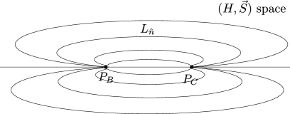
Figure 1: We can foliate the $D$-dimensional configuration space by a set of $L_{\hat{n}}$ with $\hat{n}\in S^{D-1}$ starting with $P_{B}$ and ending at $P_{C}$. Here we show the case of $D=2$, where $\hat{n}\in S^{1}$ is a point of the circle, namely specifies the direction in the neighborhood of the point $P_{B}$.

Let us fix $\hat{n}\in S^{D-1}$ and consider the function $V_{H,S}$ along the line $L_{\hat{n}}$, starting with the point $P_{B}$. Since $P_{B}$ was the EW vacuum we start with $V_{H,S}=0$, and by assumption (B) the potential grows into positive values as we gradually move along $L_{\hat{n}}$. Since we know (by assumption (C) and (A)) that the potential should reach negative values by the time we get to the point $P_{C}$, and since the potential is the continuous function of the arguments, we quickly conclude that there should be at least one local maximum along the path $L_{\hat{n}}$. If there are multiple such local maximums, we take the one closest to the point $P_{B}$, and we call this point $P_{\hat{n}}$. Obviously we find $V(P_{\hat{n}})>0$.

Let us now consider the values of the potential $V(P_{\hat{n}})$ as we change $\hat{n}\in S^{D-1}$. Since $S^{D-1}$ is a compact space, there is necessarily a point $\hat{n}_{*}\in S^{D-1}$ which attains the minimum:

$$\begin{split}V(P_{\hat{n}_{*}})=\min_{\hat{n}\in S^{D-1}}V(P_{\hat{n}})\;.\end{split}$$ (60)

Since $V(P_{\hat{n}})>0$ for all $\hat{n}\in S^{D-1}$, we in particular find that

$$\begin{split}V(P_{\hat{n}_{*}})>0\;.\end{split}$$ (61)

Moreover, we find $P_{\hat{n}_{*}}$ is a extremal point of the potential:

$$\begin{split}\nabla V(P_{\hat{n}_{*}})>0\;.\end{split}$$ (62)

Indeed, the derivative of the potential vanishes along the path $L_{\hat{n}_{*}}$ from the definition of $P_{\hat{n}_{*}}$, and vanishes along the direction of the sphere $S^{D-1}$ thanks to the definition (60); since the derivative of the potential vanishes in all the linearly-independent directions, the derivative should vanish in all the directions. The result (61) and (62) are in contradiction with our assumption. This concludes our proof.

Our result excludes many of the possible EW modifications of the Higgs potential. For example, if we have a polynomial potential $V_{H,\vec{S}}$ for complex scalars $\vec{S}$, then we generically expect many extremal points (thus satisfying (C)), so that we can conclude without any explicit computations that the potential does not satisfy our criterion. Note that the quintessence modification in (10) solves the problem by violating the condition (C).

While we discussed this result in the context of the Higgs potential, our mathematical no-go theorem can be used in other contexts, e.g. the discussion of the moduli stabilization in the the swampland conjecture (see [60] and version 2 of [9] for one-parameter version of our discussion).

References

- [1] C. Vafa, “The String landscape and the swampland”, hep-th/0509212.
- [2] H. Ooguri and C. Vafa, “On the Geometry of the String Landscape and the Swampland”, Nucl. Phys. B766, 21 (2007), hep-th/0605264.
- [3] R. D. Peccei and H. R. Quinn, “CP Conservation in the Presence of Instantons”, Phys. Rev. Lett. 38, 1440 (1977), [,328(1977)].
- [4] R. D. Peccei and H. R. Quinn, “Constraints Imposed by CP Conservation in the Presence of Instantons”, Phys. Rev. D16, 1791 (1977).
- [5] S. Weinberg, “A New Light Boson?”, Phys. Rev. Lett. 40, 223 (1978).
- [6] F. Wilczek, “Problem of Strong p and t Invariance in the Presence of Instantons”, Phys. Rev. Lett. 40, 279 (1978).
- [7] G. Obied, H. Ooguri, L. Spodyneiko and C. Vafa, “De Sitter Space and the Swampland”, arxiv:1806.08362.
- [8] P. Agrawal, G. Obied, P. J. Steinhardt and C. Vafa, “On the Cosmological Implications of the String Swampland”, Phys. Lett. B784, 271 (2018), arxiv:1806.09718.
- [9] F. Denef, A. Hebecker and T. Wrase, “The dS swampland conjecture and the Higgs potential”, arxiv:1807.06581.
- [10] N. Arkani-Hamed, L. Motl, A. Nicolis and C. Vafa, “The String landscape, black holes and gravity as the weakest force”, JHEP 0706, 060 (2007), hep-th/0601001.
- [11] H. Ooguri and C. Vafa, “Non-supersymmetric AdS and the Swampland”, Adv. Theor. Math. Phys. 21, 1787 (2017), arxiv:1610.01533.
- [12] T. D. Brennan, F. Carta and C. Vafa, “The String Landscape, the Swampland, and the Missing Corner”, arxiv:1711.00864.
- [13] M. P. Hertzberg, S. Kachru, W. Taylor and M. Tegmark, “Inflationary Constraints on Type IIA String Theory”, JHEP 0712, 095 (2007), arxiv:0711.2512.
- [14] T. Wrase and M. Zagermann, “On Classical de Sitter Vacua in String Theory”, Fortsch. Phys. 58, 906 (2010), arxiv:1003.0029, in: “Elementary particle physics and gravity. Proceedings, Corfu Summer Institute, School and Workshops on ’Standard model and beyond and standard cosmology’ and on ’Cosmology and strings: Theory - cosmology - phenomenology’, CORFU 2009, Corfu, Greece, August 30-September 13, 2009”, pp. 906-910.
- [15] U. H. Danielsson and T. Van Riet, “What if string theory has no de Sitter vacua?”, arxiv:1804.01120.
- [16] J. M. Maldacena and C. Nunez, “Supergravity description of field theories on curved manifolds and a no go theorem”, Int. J. Mod. Phys. A16, 822 (2001), hep-th/0007018, in: “Superstrings. Proceedings, International Conference, Strings 2000, Ann Arbor, USA, July 10-15, 2000”, pp. 822-855, [,182(2000)].
- [17] J. McOrist and S. Sethi, “M-theory and Type IIA Flux Compactifications”, JHEP 1212, 122 (2012), arxiv:1208.0261.
- [18] S. Sethi, “Supersymmetry Breaking by Fluxes”, arxiv:1709.03554.
- [19] B. Ratra and P. J. E. Peebles, “Cosmological Consequences of a Rolling Homogeneous Scalar Field”, Phys. Rev. D37, 3406 (1988).
- [20] C. Wetterich, “Cosmology and the Fate of Dilatation Symmetry”, Nucl. Phys. B302, 668 (1988), arxiv:1711.03844.
- [21] I. Zlatev, L.-M. Wang and P. J. Steinhardt, “Quintessence, cosmic coincidence, and the cosmological constant”, Phys. Rev. Lett. 82, 896 (1999), astro-ph/9807002.
- [22] S. Tsujikawa, “Quintessence: A Review”, Class. Quant. Grav. 30, 214003 (2013), arxiv:1304.1961.
- [23] C.-I. Chiang and H. Murayama, “Building Supergravity Quintessence Model”, arxiv:1808.02279.
- [24] N. Arkani-Hamed, L. J. Hall, C. F. Kolda and H. Murayama, “A New perspective on cosmic coincidence problems”, Phys. Rev. Lett. 85, 4434 (2000), astro-ph/0005111.
- [25] E. Witten, “Some Properties of O(32) Superstrings”, Phys. Lett. 149B, 351 (1984).
- [26] P. Svrcek and E. Witten, “Axions In String Theory”, JHEP 0606, 051 (2006), hep-th/0605206.
- [27] P. Di Vecchia and G. Veneziano, “Chiral Dynamics in the Large n Limit”, Nucl. Phys. B171, 253 (1980).
- [28] E. Witten, “Large N Chiral Dynamics”, Annals Phys. 128, 363 (1980).
- [29] G. Grilli di Cortona, E. Hardy, J. Pardo Vega and G. Villadoro, “The QCD axion, precisely”, JHEP 1601, 034 (2016), arxiv:1511.02867.
- [30] P. Di Vecchia, G. Rossi, G. Veneziano and S. Yankielowicz, “Spontaneous breaking in QCD and the axion potential: an effective Lagrangian approach”, JHEP 1712, 104 (2017), arxiv:1709.00731.
- [31] T. W. Grimm, E. Palti and I. Valenzuela, “Infinite Distances in Field Space and Massless Towers of States”, arxiv:1802.08264.
- [32] B. Heidenreich, M. Reece and T. Rudelius, “Emergence of Weak Coupling at Large Distance in Quantum Gravity”, Phys. Rev. Lett. 121, 051601 (2018), arxiv:1802.08698.
- [33] R. Blumenhagen, “Large Field Inflation/Quintessence and the Refined Swampland Distance Conjecture”, PoS CORFU2017, 175 (2018), arxiv:1804.10504, in: “Proceedings, 17th Hellenic School and Workshops on Elementary Particle Physics and Gravity (CORFU2017): Corfu, Greece, September 2-28, 2017”, pp. 175.
- [34] S.-J. Lee, W. Lerche and T. Weigand, “Tensionless Strings and the Weak Gravity Conjecture”, arxiv:1808.05958.
- [35] B. Heidenreich, M. Reece and T. Rudelius, “Sharpening the Weak Gravity Conjecture with Dimensional Reduction”, JHEP 1602, 140 (2016), arxiv:1509.06374.
- [36] B. Heidenreich, M. Reece and T. Rudelius, “Evidence for a sublattice weak gravity conjecture”, JHEP 1708, 025 (2017), arxiv:1606.08437.
- [37] D. Harlow, “Wormholes, Emergent Gauge Fields, and the Weak Gravity Conjecture”, JHEP 1601, 122 (2016), arxiv:1510.07911.
- [38] C. Cheung and G. N. Remmen, “Naturalness and the Weak Gravity Conjecture”, Phys. Rev. Lett. 113, 051601 (2014), arxiv:1402.2287.
- [39] M. Montero, G. Shiu and P. Soler, “The Weak Gravity Conjecture in three dimensions”, JHEP 1610, 159 (2016), arxiv:1606.08438.
- [40] A. R. Liddle, A. Mazumdar and F. E. Schunck, “Assisted inflation”, Phys. Rev. D58, 061301 (1998), astro-ph/9804177.
- [41] E. J. Copeland, A. Mazumdar and N. J. Nunes, “Generalized assisted inflation”, Phys. Rev. D60, 083506 (1999), astro-ph/9904309.
- [42] S. Dimopoulos, S. Kachru, J. McGreevy and J. G. Wacker, “N-flation”, JCAP 0808, 003 (2008), hep-th/0507205.
- [43] J. E. Kim, H. P. Nilles and M. Peloso, “Completing natural inflation”, JCAP 0501, 005 (2005), hep-ph/0409138.
- [44] T. Rudelius, “Constraints on Axion Inflation from the Weak Gravity Conjecture”, JCAP 1509, 020 (2015), arxiv:1503.00795.
- [45] M. Montero, A. M. Uranga and I. Valenzuela, “Transplanckian axions!?”, JHEP 1508, 032 (2015), arxiv:1503.03886.
- [46] J. Brown, W. Cottrell, G. Shiu and P. Soler, “Fencing in the Swampland: Quantum Gravity Constraints on Large Field Inflation”, JHEP 1510, 023 (2015), arxiv:1503.04783.
- [47] B. Heidenreich, M. Reece and T. Rudelius, “Weak Gravity Strongly Constrains Large-Field Axion Inflation”, JHEP 1512, 108 (2015), arxiv:1506.03447.
- [48] M. Kamionkowski and J. March-Russell, “Planck scale physics and the Peccei-Quinn mechanism”, Phys. Lett. B282, 137 (1992), hep-th/9202003.
- [49] T. A. Wagner, S. Schlamminger, J. H. Gundlach and E. G. Adelberger, “Torsion-balance tests of the weak equivalence principle”, Class. Quant. Grav. 29, 184002 (2012), arxiv:1207.2442.
- [50] V. A. Rubakov, “Grand unification and heavy axion”, JETP Lett. 65, 621 (1997), hep-ph/9703409.
- [51] Z. Berezhiani, L. Gianfagna and M. Giannotti, “Strong CP problem and mirror world: The Weinberg-Wilczek axion revisited”, Phys. Lett. B500, 286 (2001), hep-ph/0009290.
- [52] A. Hook, “Anomalous solutions to the strong CP problem”, Phys. Rev. Lett. 114, 141801 (2015), arxiv:1411.3325.
- [53] H. Fukuda, K. Harigaya, M. Ibe and T. T. Yanagida, “Model of visible QCD axion”, Phys. Rev. D92, 015021 (2015), arxiv:1504.06084.
- [54] D. Andriot, “On the de Sitter swampland criterion”, arxiv:1806.10999.
- [55] L. Aalsma, M. Tournoy, J. P. Van Der Schaar and B. Vercnocke, “A Supersymmetric Embedding of Anti-Brane Polarization”, arxiv:1807.03303.
- [56] S. K. Garg and C. Krishnan, “Bounds on Slow Roll and the de Sitter Swampland”, arxiv:1807.05193.
- [57] C. Roupec and T. Wrase, “de Sitter extrema and the swampland”, arxiv:1807.09538.
- [58] D. Andriot, “New constraints on classical de Sitter: flirting with the swampland”, arxiv:1807.09698.
- [59] L. Heisenberg, M. Bartelmann, R. Brandenberger and A. Refregier, “Dark Energy in the Swampland”, arxiv:1808.02877.
- [60] J. P. Conlon, “The de Sitter swampland conjecture and supersymmetric AdS vacua”, arxiv:1808.05040.
- [61] K. Dasgupta, M. Emelin, E. McDonough and R. Tatar, “Quantum Corrections and the de Sitter Swampland Conjecture”, arxiv:1808.07498.
- [62] S. Kachru and S. Trivedi, “A comment on effective field theories of flux vacua”, arxiv:1808.08971.
- [63] M. Cicoli, S. de Alwis, A. Maharana, F. Muia and F. Quevedo, “De Sitter vs Quintessence in String Theory”, arxiv:1808.08967.
- [64] Y. Akrami, R. Kallosh, A. Linde and V. Vardanyan, “The landscape, the swampland and the era of precision cosmology”, arxiv:1808.09440.
- [65] T. Banks, Y. Nir and N. Seiberg, “Missing (up) mass, accidental anomalous symmetries, and the strong CP problem”, hep-ph/9403203, in: “Yukawa couplings and the origins of mass. Proceedings, 2nd IFT Workshop, Gainesville, USA, February 11-13, 1994”, pp. 26-41.
- [66] S. Aoki et al., “Review of lattice results concerning low-energy particle physics”, Eur. Phys. J. C74, 2890 (2014), arxiv:1310.8555.
- [67] M. Dine, P. Draper and G. Festuccia, “Instanton Effects in Three Flavor QCD”, Phys. Rev. D92, 054004 (2015), arxiv:1410.8505.
- [68] J. Frison, R. Kitano and N. Yamada, “ mass dependence of the topological susceptibility”, PoS LATTICE2016, 323 (2016), arxiv:1611.07150, in: “Proceedings, 34th International Symposium on Lattice Field Theory (Lattice 2016): Southampton, UK, July 24-30, 2016”, pp. 323.
- [69] A. E. Nelson, “Naturally Weak CP Violation”, Phys. Lett. 136B, 387 (1984).
- [70] S. M. Barr, “Solving the Strong CP Problem Without the Peccei-Quinn Symmetry”, Phys. Rev. Lett. 53, 329 (1984).
- [71] A. Masiero and T. Yanagida, “Real CP violation”, hep-ph/9812225.
- [72] J. L. Evans, B. Feldstein, W. Klemm, H. Murayama and T. T. Yanagida, “Hermitian Flavor Violation”, Phys. Lett. B703, 599 (2011), arxiv:1106.1734.
- [73] A. Strominger and E. Witten, “New Manifolds for Superstring Compactification”, Commun. Math. Phys. 101, 341 (1985).
- [74] M. B. Green, J. H. Schwarz and E. Witten, “SUPERSTRING THEORY. VOL. 2: LOOP AMPLITUDES, ANOMALIES AND PHENOMENOLOGY”.
- [75] M. Dine, R. G. Leigh and D. A. MacIntire, “Of CP and other gauge symmetries in string theory”, Phys. Rev. Lett. 69, 2030 (1992), hep-th/9205011.
- [76] K.-w. Choi, D. B. Kaplan and A. E. Nelson, “Is CP a gauge symmetry?”, Nucl. Phys. B391, 515 (1993), hep-ph/9205202.
- [77] S. Cecotti and C. Vafa, “Theta-problem and the String Swampland”, arxiv:1808.03483.
- [78] E. Witten, “Dynamical Breaking of Supersymmetry”, Nucl. Phys. B188, 513 (1981).
- [79] K.-I. Izawa and T. Yanagida, “Dynamical supersymmetry breaking in vector - like gauge theories”, Prog. Theor. Phys. 95, 829 (1996), hep-th/9602180.
- [80] K. A. Intriligator and S. D. Thomas, “Dynamical supersymmetry breaking on quantum moduli spaces”, Nucl. Phys. B473, 121 (1996), hep-th/9603158.
- [81] K. I. Izawa, F. Takahashi, T. T. Yanagida and K. Yonekura, “Gravity Mediation of Supersymmetry Breaking with Dynamical Metastability”, arxiv:0810.5413.
- [82] K. A. Intriligator, N. Seiberg and D. Shih, “Dynamical SUSY breaking in meta-stable vacua”, JHEP 0604, 021 (2006), hep-th/0602239.
- [83] H. Murayama and Y. Nomura, “Gauge Mediation Simplified”, Phys. Rev. Lett. 98, 151803 (2007), hep-ph/0612186.
- [84] H. Murayama and Y. Nomura, “Simple Scheme for Gauge Mediation”, Phys. Rev. D75, 095011 (2007), hep-ph/0701231.
- [85] E. Witten, “Theta dependence in the large N limit of four-dimensional gauge theories”, Phys. Rev. Lett. 81, 2862 (1998), hep-th/9807109.
- [86] M. Yamazaki and K. Yonekura, “From 4d Yang-Mills to 2d model: IR problem and confinement at weak coupling”, JHEP 1707, 088 (2017), arxiv:1704.05852.
- [87] K. Aitken, A. Cherman and M. Ünsal, “Vacuum structure of Yang-Mills theory as a function of ”, arxiv:1804.06848.
- [88] I. Affleck, M. Dine and N. Seiberg, “Dynamical Supersymmetry Breaking in Supersymmetric QCD”, Nucl. Phys. B241, 493 (1984).
- [89] R. F. Dashen, “Some features of chiral symmetry breaking”, Phys. Rev. D3, 1879 (1971).
- [90] A. Achücarro and G. A. Palma, “The string swampland constraints require multi-field inflation”, arxiv:1807.04390.
- [91] A. Kehagias and A. Riotto, “A note on Inflation and the Swampland”, arxiv:1807.05445.
- [92] H. Matsui and F. Takahashi, “Eternal Inflation and Swampland Conjectures”, arxiv:1807.11938.
- [93] I. Ben-Dayan, “Draining the Swampland”, arxiv:1808.01615.
- [94] W. H. Kinney, S. Vagnozzi and L. Visinelli, “The Zoo Plot Meets the Swampland: Mutual (In)Consistency of Single-Field Inflation, String Conjectures, and Cosmological Data”, arxiv:1808.06424.
- [95] N. Kaloper, A. Lawrence and L. Sorbo, “An Ignoble Approach to Large Field Inflation”, JCAP 1103, 023 (2011), arxiv:1101.0026.
- [96] S. Dubovsky, A. Lawrence and M. M. Roberts, “Axion monodromy in a model of holographic gluodynamics”, JHEP 1202, 053 (2012), arxiv:1105.3740.
- [97] M. Dine, P. Draper and A. Monteux, “Monodromy Inflation in SUSY QCD”, JHEP 1407, 146 (2014), arxiv:1405.0068.
- [98] K. Yonekura, “Notes on natural inflation”, JCAP 1410, 054 (2014), arxiv:1405.0734.
- [99] N. Kaloper and A. Lawrence, “London equation for monodromy inflation”, Phys. Rev. D95, 063526 (2017), arxiv:1607.06105.
- [100] E. Silverstein and A. Westphal, “Monodromy in the CMB: Gravity Waves and String Inflation”, Phys. Rev. D78, 106003 (2008), arxiv:0803.3085.
- [101] L. McAllister, E. Silverstein and A. Westphal, “Gravity Waves and Linear Inflation from Axion Monodromy”, Phys. Rev. D82, 046003 (2010), arxiv:0808.0706.
- [102] Y. Nomura, T. Watari and M. Yamazaki, “Pure Natural Inflation”, arxiv:1706.08522.
- [103] K. Freese, J. A. Frieman and A. V. Olinto, “Natural inflation with pseudo - Nambu-Goldstone bosons”, Phys. Rev. Lett. 65, 3233 (1990).
- [104] L. Giusti, S. Petrarca and B. Taglienti, “Theta dependence of the vacuum energy in the SU(3) gauge theory from the lattice”, Phys. Rev. D76, 094510 (2007), arxiv:0705.2352.
- [105] Y. Nomura and M. Yamazaki, “Tensor Modes in Pure Natural Inflation”, Phys. Lett. B780, 106 (2018), arxiv:1711.10490.