The ice composition in the disk around V883 Ori revealed by its stellar outburst
Abstract
Complex organic molecules (COMs), which are the seeds of prebiotic material and precursors of amino acids and sugars, form in the icy mantles of circumstellar dust grains[1] but cannot be detected remotely unless they are heated and released to the gas phase. Around solar-mass stars, water and COMs only sublimate in the inner few au of the disk[2], making them extremely difficult to spatially resolve and study. Sudden increases in the luminosity of the central star will quickly expand the sublimation front (so-called snow line) to larger radii, as seen previously in the FU Ori outburst of the young star V883 Ori[3]. In this paper, we take advantage of the rapid increase in disk temperature of V883 Ori to detect and analyze five different COMs, methanol, acetone, acetonitrile, acetaldehyde, and methyl formate, in spatially-resolved submillimeter observations. The COMs abundances in V883 Ori is in reasonable agreement with cometary values[4]. This result suggests that outbursting young stars can provide a special opportunity to study the ice composition of material directly related to planet formation.
School of Space Research, Kyung Hee University, 1732, Deogyeong-Daero, Giheung-gu, Yongin-shi, Gyunggi-do 17104, Korea
Department of Astronomy, University of Tokyo, 7-3-1 Hongo, Bunkyo-ku, Tokyo 113-0033, Japan
Facultad de Ingeniería y Ciencias, Núcleo de Astronomía, Universidad Diego Portales, Av. Ejercito 441. Santiago, Chile
Kavli Institute for Astronomy and Astrophysics, Peking University, Yi He Yuan Lu 5, Haidian Qu, 100871, Beijing, PR China
NRC Herzberg Astronomy and Astrophysics, 5071 West Saanich Road, Victoria, BC, V9E 2E7, Canada
Departamento de Astronomía, Universidad de Chile, Casilla 36-D Santiago, Chile
Observations of comets and asteroids show that the Solar nebula was rich in water and organic molecules. The inventory from the recent Rosetta mission to comet 67P/Churyumov–Gerasimenko includes many complex organic molecules (COMs)[5] as well as prebiotic molecules. These organics, together with water, could have been brought to the young Earth’s surface by comets[6]. Since the ice composition of comets is similar to ices in molecular clouds, it has long been debated if cometary ices originate in the interstellar matter (ISM). The evolution of volatiles during planet formation may be traced by comparing the abundances from the youngest phases of star and disk formation, the protostellar core phase (when the star and disk are still growing from a circumstellar envelope), to the older phases of disk evolution. The Atacama Large Millimeter/submillimeter Array (ALMA) revealed that in some protostellar cores, called hot corinos, the warm gas contains various COMs that are also detected in comets[7, 8]. The variation of chemical composition among comets[4], however, suggests that chemical processes could be active even after material from the ISM is incorporated to the disk[9]. The chemical reactions, in turn, depend on various physical parameters in the disk, e.g. ionization rate and dust-gas decoupling, which are under debate[10, 11].
Despite efforts to observe ices in disks, clear detection of ices in the disk midplane is challenging and requires sophisticated analysis that considers the inclination angle and foreground contamination[12]. An alternative approach is to observe COMs in the gas phase inside the snow line, defined as the radius outside of which a molecule is predominantly in ice form. The location of each snow line depends on the heating of the disk by the central star and by the release of gravitational energy via mass accretion, as well as on the sublimation temperature of the molecule[13]. However, for a typical disk around a solar-mass star and a mass accretion rate of M⊙ yr-1, the COM and water snow lines are located at a radius of only a few AU[2], too small to be spatially resolved even with ALMA. So far, three gaseous COMs, CH3OH, CH3CN, and HCOOH, have been detected in non-bursting protoplanetary disks[14, 15, 16, 17, 18], with emission that traces non-thermally desorbed molecules in the outer (10 AU) disk surface, far beyond the snow line. Derivation of solid-phase abundances from those observations is not straightforward; it needs detailed understanding of the non-thermal desorption mechanisms and of gas-phase reactions that could change the abundances after desorption[19].
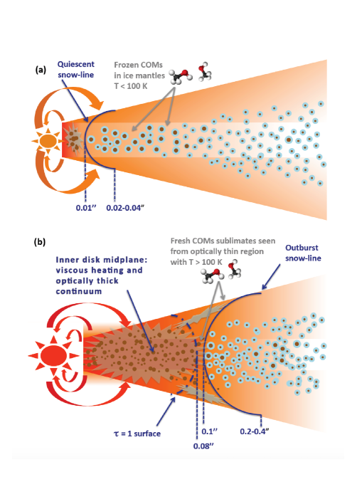
The abundances of COMs at the disk locations where icy planetesimals form may instead be best measured during a protostellar outburst[20], which viscously heats the disk and extends snow line to a much larger radius. The gas emission from the freshly sublimated COMs should directly trace the abundances of COMs that were previously in the ice phase. FUors are young stellar objects that exhibit large-amplitude outbursts in the optical (change in magnitude mag) and undergo rapid increases of accretion rate, by 3 orders of magnitude (from to M⊙ yr-1)[21]. The high luminosity due to the enhanced accretion rate shifts the snow line to much larger radii[22]. For the FUor outburst V883 Ori studied here, the radius of the water snow line at the disk midplane is estimated to be 40 AU from 1.3 mm continuum emission[3]; the snow line at the disk surface may extend to 160 AU. Theoretical studies show that the sublimates are destroyed by the gas-phase reactions in several 104 yr[23]. Since the duration of a typical outburst is usually 100 years, FUors provide a unique and direct probe to study the composition of fresh sublimates of COMs located in the disk midplane, which were in ice form in the pre-burst phase. When the outburst stops, the dust grains will cool instantaneously, so these COMs will be frozen back onto grain surfaces within one year (see Methods).
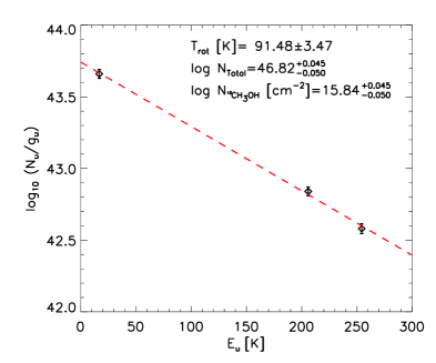
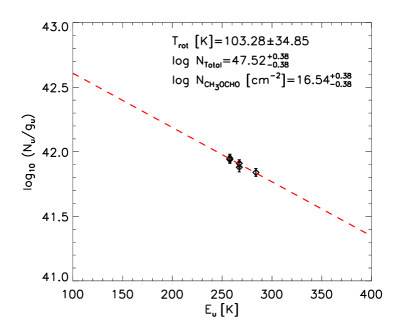
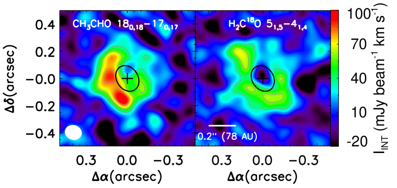
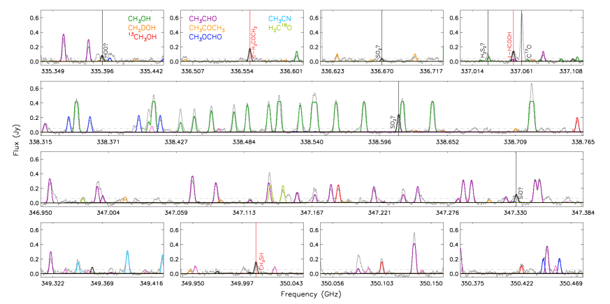
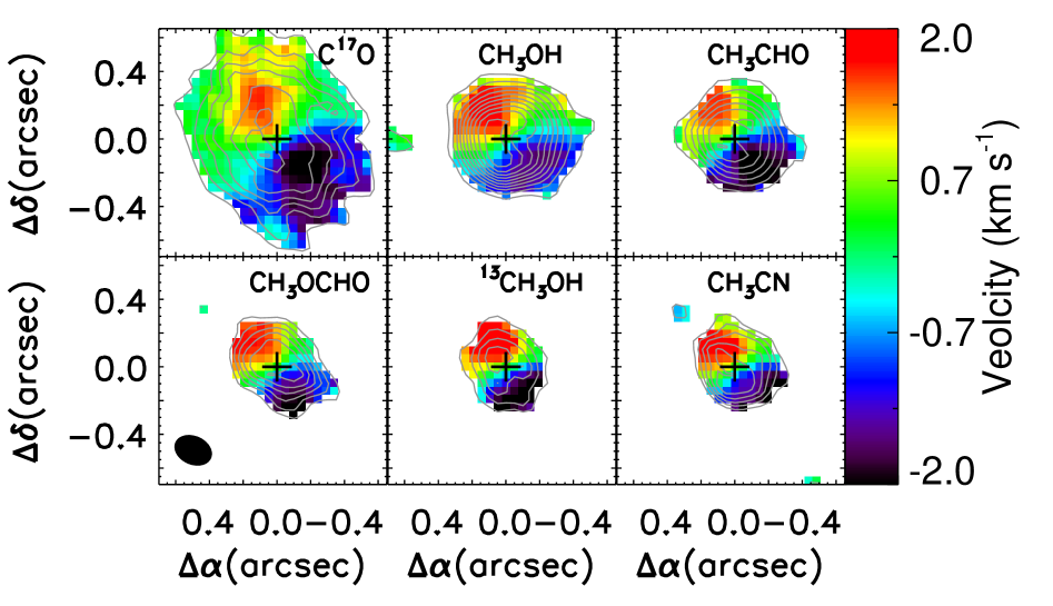
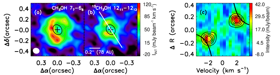
We observed V883 Ori, a FU Ori star with mass of 1.2 M⊙[3] (see Methods), with ALMA in Band 7 on 8 September 2017 with a resolution of , designed for continuum images, and on 21 February 2018 with a resolution of , designed to measure COM emission. From the lower-resolution observation, we detected many COMs lines, including CH3CHO, CH3OCHO, and CH3COCH3, which are robustly detected for the first time in protoplanetary disks (Figure 1). CH3CHO and CH3OCHO were detected contemporaneously and independently in the same target[24]. Figure 2 shows the integrated intensity images (contours) and intensity weighted velocity images (colors) of emission coadded in many lines of individual COMs from the lower-resolution observation. All COM emission is confined within 0.4′′, but the emission peaks are offset from the continuum peak. We find excitation temperatures for 13CH3OH of 91.5 3.5 K and for CH3OCHO of 103.3 34.9 K (see Supplementary Figure 1). The lines of these two molecules are reasonably optically thin (line optical depth , see Methods).
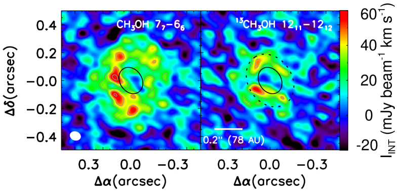
While the high resolution data was obtained to image the dust continuum, it also contains some COMs emissions. The high-resolution images (Figure 3 and Supplementary Figures 2 and 3) reveal that the COM emission originates in a ring region around the water snow line that was previously identified from the dust continuum observations. The 13CH3OH emission arises only between 0.1′′-0.2′′, in contrast to the expectation that COMs emission should be bright inside the snow line. The position-velocity map presented in Figure 3(c) is reproduced well by ring within a Keplerian disk, consistent with the CO emission[3].
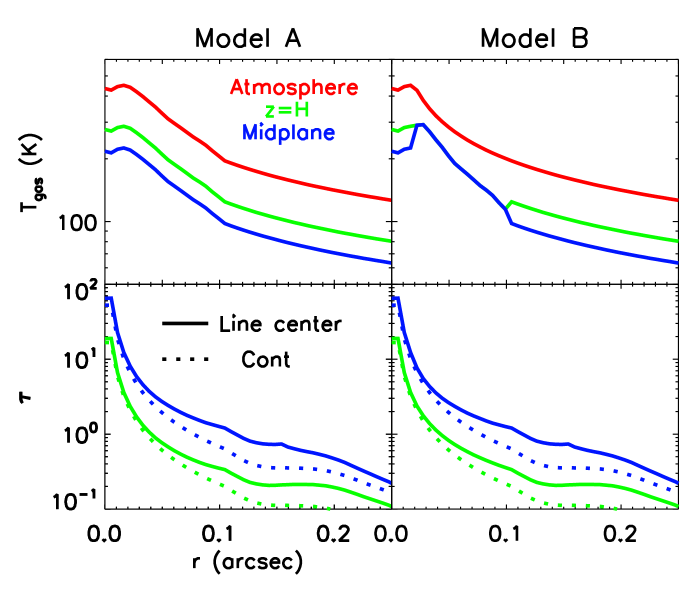
Disks are heated by stellar irradiation and viscous accretion[2, 25]. When stellar irradiation dominates, then the disk surface is warmer than the midplane, while the midplane could be warmer when the accretion heating dominates. The location where the water sublimates thus varies both with the distance from the star and with the height from the midplane, which together defines the snow surface (Supplementary Figure 5). Because the molecular line opacity tends to be higher than that of the dust continuum, the 2-D (radial and vertical) temperature distribution is needed to analyze molecular line emission.
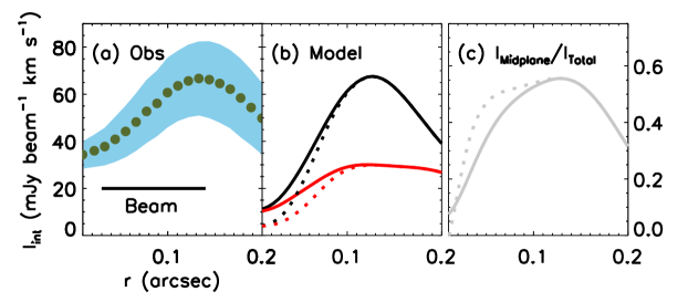
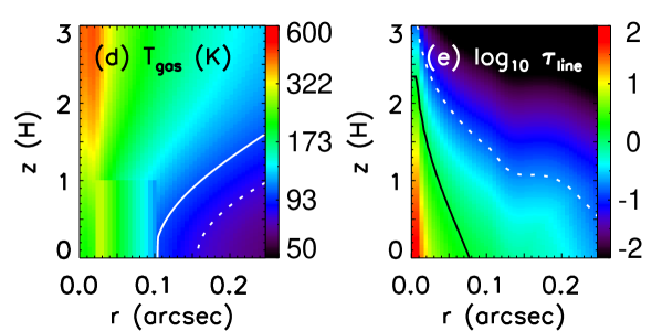
Since heating by irradiation and accretion are both important for FUors[26], we tested two models for the optically thin 13CH3OH line emission: Model A for the disk heated only by irradiation and Model B for the disk heated by an enhanced accretion in the midplane as well as irradiation (see Methods and Supplementary Figure 4 for the details of models). Figure 4 compares the results of the two models with the observed emission distribution of 13CH3OH . The observed emission decreases inside of its snow line, which is well reproduced by Model A and is a consequence of increasing dust continuum optical depths (see the bottom panels of Figure 4 and Supplementary Figures 4) caused by the evaporation of cm-sized icy pebbles (containing micron-sized dust grains) and the re-coagulation of the bare silicates into submm-sized grains[27]. In Model B, the 13CH3OH emission declines even more steeply inwards due to the self-absorption caused by the negative temperature gradient in the vertical direction. Observations with higher spatial resolution and better sensitivity are needed to discriminate between these two models. Figure 4 also compares the total amount of 13CH3OH emission with that produced in the disk surface. The fraction of emission from the midplane reaches a maximum near the methanol snow line, confirming that the COM compositions in the gas phase originate in the ice compositions in the midplane regions that are likely forming planetesimals.
The average column densities of COMs over their emitting area are derived by fitting the observed spectra (Figure 1) with XCLASS[28] (Supplementary Table 1). The abundances with respect to molecular hydrogen are times higher than those derived from the spatially-extended COMs emission of non-bursting disks ()[14, 15, 16, 17, 18], confirming that our observations probe the thermal sublimation of COMs. The D/H and 13C/12C ratios of CH3OH are 0.16 and 0.13, which are significantly higher than the ratios in protostellar cores and elemental abundances. While the high D/H ratio could be due to deuterium fractionation in the dense and cold grain surfaces[13], the high 13C/12C ratio indicates that the column density of CH3OH is underestimated due to the high optical depth of the lines, requiring a more detailed treatment than that taken by XCLASS. We thus assume that the actual column density of CH3OH is equal to that of 13CH3OH multiplied by the elemental abundance of 12C/13C (see Methods).
We find most COMs abundances relative to CH3OH, i.e. their column density ratios, are higher than those in the hot corino IRAS 16293 B[8, 29, 30]; the abundances of CH3COCH3, CH3CHO, and CH3OCHO are higher than those in IRAS 16293 B by factors of 4 to 16 (Supplementary Table 1). The abundances of CH3COCH3 and CH3CHO in both V883 Ori and IRAS 16293 B agree with those in comet 67P/Churyumov–Gerasimenko[4, 9] by a factor of a few. Acetone is not detected by by the Rosetta Orbiter Spectrometer for Ion and Neutral Analysis (ROSINA) on board Rosetta but was estimated to be as abundant as CH3CHO in 67P/Churyumov–Gerasimenko by the Cometary Sampling and Composition Experiment (COSAC)[1], which could be in reasonable agreement with V883 Ori. CH3CN abundance in V883 Ori, on the other hand, is lower than in IRAS 16293 B (comets) by a factor of 3 (an order of magnitude). The CH3CN/CH3OH abundance ratio is also much lower than that in cold vapor in outer radii of other disks (1)[16, 17]. These abundances indicate that formation and destruction of COMs continue after the volatiles are incorporated to the disk.
Our observations and analysis of V883 Ori demonstrate that observations of FUors are unique in revealing fresh sublimates and thus ice composition in protoplanetary disks. Although FUors are rare, they span a range of evolutionary states: some outbursts occur while the system is still being fed by their envelope, other outbursts occur in systems that have only disks and no envelope[21]. This diversity may provide us with the leverage to investigate how the chemical evolution of complex molecules in protoplanetary disks leaves its imprints on the products of planet formation.
References
- [1] Herbst, E. & van Dishoeck, E. F. Complex Organic Interstellar Molecules. ARA&A 47, 427–480 (2009).
- [2] D’Alessio, P., Calvet, N. & Hartmann, L. Accretion Disks around Young Objects. III. Grain Growth. ApJ 553, 321–334 (2001). astro-ph/0101443.
- [3] Cieza, L. A. et al. Imaging the water snow-line during a protostellar outburst. Nature 535, 258–261 (2016). 1607.03757.
- [4] Le Roy, L. et al. Inventory of the volatiles on comet 67P/Churyumov-Gerasimenko from Rosetta/ROSINA. A&A 583, A1 (2015).
- [5] Altwegg, K. et al. Organics in comet 67P - a first comparative analysis of mass spectra from ROSINA-DFMS, COSAC and Ptolemy. MNRAS 469, S130–S141 (2017).
- [6] Chyba, C. F., Thomas, P. J., Brookshaw, L. & Sagan, C. Cometary Delivery of Organic Molecules to the Early Earth. Science 249, 366–373 (1990).
- [7] Imai, M. et al. Discovery of a Hot Corino in the Bok Globule B335. ApJ 830, L37 (2016). 1610.03942.
- [8] Jørgensen, J. K. et al. The ALMA Protostellar Interferometric Line Survey (PILS). First results from an unbiased submillimeter wavelength line survey of the Class 0 protostellar binary IRAS 16293-2422 with ALMA. A&A 595, A117 (2016). 1607.08733.
- [9] Mumma, M. J. & Charnley, S. B. The Chemical Composition of CometsEmerging Taxonomies and Natal Heritage. ARA&A 49, 471–524 (2011).
- [10] Furuya, K. & Aikawa, Y. Reprocessing of Ices in Turbulent Protoplanetary Disks: Carbon and Nitrogen Chemistry. ApJ 790, 97 (2014). 1406.3507.
- [11] Schwarz, K. R. et al. Unlocking CO Depletion in Protoplanetary Disks. I. The Warm Molecular Layer. ApJ 856, 85 (2018). 1802.02590.
- [12] Pontoppidan, K. M. et al. Ices in the Edge-on Disk CRBR 2422.8-3423: Spitzer Spectroscopy and Monte Carlo Radiative Transfer Modeling. ApJ 622, 463–481 (2005). astro-ph/0411367.
- [13] Hama, T. & Watanabe, N. Surface Processes on Interstellar Amorphous Solid Water: Adsorption, Diffusion, Tunneling Reactions, and Nuclear-Spin Conversion. Chem. Rev. 113, 8783–8839 (2013).
- [14] Walsh, C. et al. First Detection of Gas-phase Methanol in a Protoplanetary Disk. ApJ 823, L10 (2016). 1606.06492.
- [15] i̱binfoauthorÖberg, K. I. et al. The comet-like composition of a protoplanetary disk as revealed by complex cyanides. Nature 520, 198–201 (2015). 1505.06347.
- [16] Loomis, R. A. et al. Detecting Weak Spectral Lines in Interferometric Data through Matched Filtering. AJ 155, 182 (2018). 1803.04987.
- [17] Bergner, J. B., Guzmán, V. G., bibinfoauthorÖberg, K. I., Loomis, R. A. & Pegues, J. A Survey of CH3CN and HC3N in Protoplanetary Disks. ApJ 857, 69 (2018). 1803.04986.
- [18] Favre, C. et al. First Detection of the Simplest Organic Acid in a Protoplanetary Disk. ApJ 862, L2 (2018). 1807.05768.
- [19] Bertin, M. et al. UV Photodesorption of Methanol in Pure and CO-rich Ices: Desorption Rates of the Intact Molecule and of the Photofragments. ApJ 817, L12 (2016). 1601.07027.
- [20] Molyarova, T. et al. Chemical Signatures of the FU Ori Outbursts. ApJ 866, 46 (2018). 1809.01925.
- [21] Audard, M. et al. Episodic Accretion in Young Stars. Protostars and Planets VI 387–410 (2014). 1401.3368.
- [22] Harsono, D., Bruderer, S. & van Dishoeck, E. F. Volatile snowlines in embedded disks around low-mass protostars. A&A 582, A41 (2015). 1507.07480.
- [23] Nomura, H., Aikawa, Y., Nakagawa, Y. & Millar, T. J. Effects of accretion flow on the chemical structure in the inner regions of protoplanetary disks. A&A 495, 183–188 (2009). 0810.4610.
- [24] van ’t Hoff, M. L. R. et al. Methanol and its Relation to the Water Snowline in the Disk around the Young Outbursting Star V883 Ori. ApJ 864, L23 (2018). 1808.08258.
- [25] Qi, C. et al. CO J = 6-5 Observations of TW Hydrae with the Submillimeter Array. ApJ 636, L157–L160 (2006). astro-ph/0512122.
- [26] Dullemond, C. P., Hollenbach, D., Kamp, I. & D’Alessio, P. Models of the Structure and Evolution of Protoplanetary Disks. Protostars and Planets V 555–572 (2007). astro-ph/0602619.
- [27] Schoonenberg, D., Okuzumi, S. & Ormel, C. W. What pebbles are made of: Interpretation of the V883 Ori disk. A&A 605, L2 (2017). 1708.03328.
- [28] Möller, T., Endres, C. & Schilke, P. eXtended CASA Line Analysis Software Suite (XCLASS). A&A 598, A7 (2017). 1508.04114.
- [29] Lykke, J. M. et al. The ALMA-PILS survey: First detections of ethylene oxide, acetone and propanal toward the low-mass protostar IRAS 16293-2422. A&A 597, A53 (2017). 1611.07314.
- [30] Calcutt, H. et al. The ALMA-PILS survey: first detection of methyl isocyanide (CHNC) in a solar-type protostar. A&A 617, A95 (2018). 1807.02909. {addendum} Correspondence and requests for materials should be addressed to Jeong-Eun Lee (email: jeongeun.lee@khu.ac.kr). ALMA is a partnership of ESO (representing its member states), NSF (USA) and NINS (Japan), together with NRC (Canada), NSC and ASIAA (Taiwan), and KASI (Republic of Korea), in cooperation with the Republic of Chile. The Joint ALMA Observatory is operated by ESO, AUI/NRAO and NAOJ. J.-E.L. is supported by the Basic Science Research Program through the National Research Foundation of Korea (grant no. NRF- 2018R1A2B6003423) and the Korea Astronomy and Space Science Institute under the R&D programme supervised by the Ministry of Science, ICT and Future Planning. G.H. is funded by general grant 11473005 awarded by the National Science Foundation of China. D.J. is supported by the National Research Council of Canada and by an NSERC Discovery Grant. Y.A. acknowledges support from JSPS KAHENHI grant numbers 16K13782 and 18H05222. J.-E.L., S.L. and G.B. performed the detailed calculations and line fittings used in the analysis. J.-E.L. wrote the manuscript. All authors were participants in the discussion of results, determination of the conclusions and revision of the manuscript. The authors declare that they have no competing financial interests.
Methods
ALMA observations
V883 Ori was observed using the Atacama Large Millimeter/submillimeter Array (ALMA) during Cycle 4 (2016.1.00728.S, PI: Lucas Cieza) on 2017 Sep. 8 and during Cycle 5 (2017.1.01066.T, PI: Jeong-Eun Lee) on 2018 Feb. 21. For the Cycle 4 observation, a spectral window was centered at 334.3955GHz (HDO 33,1-42,2) with a bandwidth of 93.75 MHz and spectral resolution of 488 kHz (v km s-1). Three windows used for continuum, centered at 333.41 GHz, 345.41 GHz, and 347.41 GHz with a bandwidth of 2 GHz, are not analyzed in this paper. The phase center was at , and the total observing time was 15.6 minutes. Forty-seven 12-m antennas were used with baselines in the range from 21 m (24 k) to 10.6 km (11900 k) to provide the synthesized beam size of (PA=) when Briggs weighting (robust = 0.5) is adopted. For the Cycle 5 observation, ten spectral windows were set to cover many molecular lines such as CH3OH, 13CH3OH, H13CO+ , and C17O . Their bandwidths were 468.75 MHz or 117.19 MHz and their spectral resolution was 282 kHz (0.2 km s-1). The total observing time was 44.53 minutes. The phase center was at . Forty-five 12-m antennas were used with baselines in the range from 15 m (17 k) to 1.4 km (1578 k) to provide the synthesized beam size of (PA=) when Briggs weighting (robust = 0.0) is adopted.
We carried out the standard data reduction using CASA 4.7.2 (for Cycle 4) and 5.1.1 (for Cycle 5) [2]. For the Cycle 4 data, the nearby quasar J0541-0541 was used for phase calibration, J0503-1800 for bandpass calibration, and J0423-0120 for flux calibration. For the Cycle 5 data, J0607-0834 was used for phase calibration while J0510+1800 was used for bandpass and flux calibration. For the Cycle 4 data, Briggs weighting with a uv-taper of 1000 k was used for the molecular lines to obtain images with a higher signal-to-noise ratio and a resolution (, PA=), enough to resolve the water snow line. The root mean square (RMS) noise level of the molecular lines is 4 mJy beam-1. For the Cycle 5 data, the RMS noise level for the molecular lines is 78 mJy beam-1. We did not use a uv-taper for the Cycle 5 data.
Distance to V883 Ori
V883 is a member of the L1641 cluster[3]. A cross-match between the sample of L1641 members[4] and the Gaia DR2 objects[5, 6] yields 47 stars with parallaxes accurate to at least 5%, have Gaia -band photometry brighter than 19 mag, are located within 0.5 deg of V883 Ori, and have a proper motion within 1 mas/yr of the average proper motion of the cluster. (The spatial and proper motion cuts are important because the Gaia DR2 astrometry reveals that the L1641 members[4] include at least two distinct clusters located at different distances.) This set of stars has a distance of pc and a standard deviation of 16 pc, roughly consistent with previous a Gaia DR2 analysis[7] . This standard deviation could be explained by either a real scatter of 12 pc in the distances or by underestimated errors in the parallax measurements.
The Gaia DR2 parallax of V883 Ori yields a distance of pc, and a proper motion that is highly discrepant with the L1641 cluster. If these values are correct, then V883 Ori could not be a member of L1641 or any other known young cluster. Moreover, the Gaia DR2 catalog flags the astrometric solution of V883 Ori as unreliable, which is not surprising for a variable young star. We therefore adopt the median distance to the nearby stars in L1641 of 388 pc for V883 Ori. With this updated distance, the midplane snow line is located at 39 AU rather than 42 AU[3] and the mass of the central star is 1.2 M⊙[3].
Line Identification and Fitting
In Figure 1, all lines were extracted with the circular aperture of 0.6′′, within which the signal-to-noise ratio of 13CH3OH integrated intensity is above 5. The line central velocity at each pixel within the aperture, which is affected by the disk rotation, is shifted to the source velocity to reduce the line blending[8]. The source velocity is 4.3 km s-1[3]. We identify spectral line transitions (see Supplementary Table 3) and fit the spectra using the eXtended CASA Line Analysis Software Suite (XCLASS)[28], which accesses the Cologne Database for Molecular Spectroscopy (CDMS)[9, 10] and Jet Propulsion Laboratory (JPL)[11] molecular databases. We still have several unidentified line transitions. In addition, only one transition was detected for each of -H2COCH2, -HCOOH, and CH3SH.
XCLASS takes into account the line opacity and line blending in the assumption of local thermodynamic equilibrium (LTE). The main parameters used to fit lines in XCLASS are the emission size, the excitation temperature, the column density of the species, the line full width at half maximum (FWHM), and the velocity offset with respect to the systemic velocity of the object. The aperture size (0.6′′) was adopted as the emission size. There is no velocity offset because all lines were shifted to the source velocity before combined. All lines are assumed to be Gaussian profiles with a FWHM fixed at 2 km s-1, the average value of all lines when allowed to vary. The excitation temperature of 120 K is adopted from the disk model below; the temperature was averaged within a radius of 0.3′′ in the model. With these parameters, we used MAGIX (Modeling and Analysis Generic Interface for eXternal numerical codes)[12] to optimize the fit and find the best solution.
The observational uncertainty is dominated by the absolute calibration error of 10 %. The COMs column densities derived from this line fitting are summarized in Supplementary Table 1. The error of the column density is calculated by taking absolute calibration uncertainty and fitting error into consideration. The derived column density of 13CH3OH is larger than that from the excitation diagram (Supplementary Figure 1) by a factor of 7.6. This may be caused by the continuum opacity rather than the optical depths of the 13CH3OH lines, which are optically thin according to the XCLASS fitting. The line intensity is scaled by , where is the continuum optical depth, and in band 7 at 0.1′′. This continuum optical depth effect is taken into account in XCLASS but not in the excitation diagram.
The derived column density of CH3OH suggests a very low 12C/13C ratio of 7.6, which is much lower than the typical ISM value (60)[13]. The best-fit column density of CH3OH might be underestimated as the modeled lines at the frequency range of 338.42 to 338.48 GHz are weaker than the observed ones. If we increase the column density by a factor of 2, those lines are fitted better. However, this column density does not fit the rest of lines, and it cannot increase the isotopic ratio to the normal value either. This low isotopic ratio between CH3OH and 13CH3OH may be caused by very high optical depth of CH3OH, which prevents the CH3OH lines from tracing the matter close to the midplane. Alternatively, the 2-D structures of temperature, density, and abundance could be the main reason. The XCLASS fitting of the spectra in Figure 1 is not perfect; the model spectra deviate from the observation for some other lines as well as those methanol lines. It indicates the need for more sophisticated modeling considering the 2-D distributions of temperature, density, and molecular abundances. We postpone such modeling to future work, since our high spatial resolution data cover only a limited number of lines (see Supplementary Table 2).
We also list the COM abundances with respect to CH3OH to compare with the values in the hot corino IRAS 16293B and in comets. In the calculation of the COMs abundances in V883 Ori, we assume that the true column density of CH3OH is the column density of 13CH3OH multiplied by the elemental abundance of 12C/13C[13]. The 12C/13C ratio in CH3OH is expected to be similar to the ratio in CO because CH3OH forms mainly via hydrogenation of CO on grain surfaces [14]. Since CO is the dominant carbon carrier, it is reasonable to assume 12CO/13CO=60. The 12CO/13CO ratio of 7115 measured directly from CO ices in star forming regions[15] is also similar to the elemental ratio. The CH3OH abundance derived from the 13CH3OH abundance and the 12C/13C ratio of 60 is then , which is in reasonable agreement with the recent study ()[24].
As listed in Supplementary Table 1, the COMs abundances relative to CH3OH are higher than those in the hot corino IRAS 16293 B and similar to those in comets, except for CH3CN. This pattern is indicative of chemical evolution in the disk that continues after the ISM material is incorporated to the disk. During the quiescent phase, for example, methyl formate (CH3OCHO) can form via grain-surface reactions of HCO and CH3O in the disk midplane[16]. However, it is difficult to compare directly our observational results with the chemical models because there are still many uncertainties in the grain surface reactions, such as the branching ratios of radical-radical reactions.
Models
In order to investigate the 2-D (r and z) distribution of CH3OH from our high spatial resolution data, we construct a simple irradiated disk model to calculate the radiative transfer of the 13CH3OH 1211-1212 line in the assumption of LTE. The gas is assumed to be well coupled with dust grains in the region where the 13CH3OH line forms, and thus, the gas temperature is the same as the dust temperature. We assume that the gas to dust mass ratio is constant as 100 over the entire disk. The vertical density profile in the disk is given as
| (1) |
with the H2 column density, and the scale height, . For the vertical temperature distribution, we follow the vertical gradient prescription of an irradiated disk model[17, 18]:
| (2) | |||||
with the temperature at the atmosphere, and that at the midplane, . For simplicity, we assume that is 2 based on the dust continuum radiative transfer model for V883 Ori [19].
To find and , we solve a dust continuum radiative transfer for the high resolution ALMA continuum image at Band 6:
| (3) |
with
| (4) | |||||
where is the dust absorption opacity at 1.3 mm ()[19], is the molecular hydrogen mass, and is the gas to dust mass ratio.
A previous study[3] shows that V883 Ori has a very optically thick inner disk and a optically thin outer disk. The boundary, that is located at 0.1′′, is interpreted as water snow line. In the inner disk, the dust temperature is relatively well constrained while the dust temperature and the column density are degenerate in the optically thin outer disk. Therefore, we analyze the inner and outer disks separately. At 0.1′′, we assume that follows the profile of , as used in the irradiated disk[20]. We adopt K (ref. [3]) based on the temperature estimated in the optically thick region. Given temperature distribution, can be derived by solving above equations. The derived column density at is cm-2 and the density at the midplane is cm-3 when is 0.1. At this density, the freeze-out timescale of COMs is shorter than a year if the temperature is lower than the sublimation temperature[21]. To derive the temperature profile at the inner disk (), is set to be . Here, we adopt , a typical power index of the surface density profile in the disk[27]. The temperature distribution in this disk model (Model A, hereinafter) is shown in Supplementary Figure 4.
For the synthetic 13CH3OH line emission, the continuum absorption coefficient is considered as a function of frequency, = with the spectral index of in the entire disk. The total absorption coefficient is given by
| (5) | |||||
where is the speed of light, and are the frequency and the Einstein coefficient of the transition, respectively, () and () is the level population and statistical weight in the upper (lower) energy state, respectively. (= ; in cm s-1) is the full width at half maximum of the line profile, is the velocity shift from the source velocity, is the partition function, and is the molecular abundance of 13CH3OH. We adopted km s-1, which is the average value over all lines, and , which reproduces the observed peak intensity. When is lower than the sublimation temperature, the molecule is assumed to be frozen onto grain surfaces, depleted from the gas. The sublimation temperature of 13CH3OH, which fits the radial intensity profile, was 80 K, as marked with the white dashed line in Figure 4(d); above the dashed line, , but below the line, . This lower sublimation temperature of CH3OH than water sublimation temperature is consistent with the lower binding energy (5000 K) of CH3OH than that of water (5600 K)[22]. The molecular data are adopted from CDMS database[9].
Finally, the line emission is synthesized using the equation (3), but with the total absorption coefficient, , instead of . The calculated intensity profile is smoothed to have the same resolution (0.11′′) of the observed image. To check whether the molecular line can trace down to the midplane, we also calculated a model in which the CH3OH abundance is artificially set to be zero in the midplane () (red lines in Figure 4); the difference between the black and red lines can be considered the emission from the disk midplane. The fraction of emission from the disk midplane is presented by the gray lines in Figure 4.
The spectral index derived from the high resolution Band 7 and Band 6 continuum images of V883 Ori is smaller than 2, reaching down to 1, within (Cassasus et al. in prep.). In the submillimeter regime, the free-free emission is negligible, and thus, most flux is likely from thermal emission, whose spectral index must be greater than 2. Note that we can see a deeper region in Band 6 than in Band 7. Thus, the flux ratio of Band 7 to Band 6 smaller than expected from the isothermal case suggests that the deeper region is hotter. Therefore, we model the disk heated by accretion (at ) as well as irradiation (Model B).
In Model B, to combine the two heating processes, irradiation and accretion, in a simple way, we assume that and are the same as those of Model A, except for the temperature distribution within the snow line. Within the snowline (), we assume that the midplane is vertically isothermal at (accretion heating), while the temperature gradient is given by Equation (2) at (irradiative heating). In Equation (2), which describes the temperature profile resulted by irradiation, we assume as used for . In Model A at a given radius, one temperature was found to fit the continuum intensity. Therefore, if at a given radius, the calculated by the above equation is lower than in Model A, then a higher midplane temperature (the blue line in the upper right panel in Supplementary Figure 4) is found to fit the observed intensity. The derived temperature distribution of Model B is presented in Figure 4(d).
This paper makes use of the ALMA data, which could be downloaded from the ALMA archive (https://almascience.nao.ac.jp/aq/) with project codes 2016.1.00728.S and 2017.1.01066.T. The data that support the plots within this paper and other findings of this study are available from the corresponding author upon reasonable request.
References
- [1] Goesmann, F. et al. Organic compounds on comet 67P/Churyumov-Gerasimenko revealed by COSAC mass spectrometry. Science 349 (2015).
- [2] McMullin, J. P., Waters, B., Schiebel, D., Young, W. & Golap, K. CASA Architecture and Applications. In Shaw, R. A., Hill, F. & Bell, D. J. (eds.) Astronomical Data Analysis Software and Systems XVI, vol. 376 of Astronomical Society of the Pacific Conference Series, 127 (2007).
- [3] Allen, L. E. & Davis, C. J. Low Mass Star Formation in the Lynds 1641 Molecular Cloud. In Reipurth, B. (ed.) Handbook of Star Forming Regions, Volume I, 621 (2008).
- [4] Fang, M. et al. Young Stellar Objects in Lynds 1641: Disks, Accretion, and Star Formation History. ApJS 207, 5 (2013). 1304.7777.
- [5] Gaia Collaboration et al. The Gaia mission. A&A 595, A1 (2016). 1609.04153.
- [6] Gaia Collaboration et al. Gaia Data Release 2. Summary of the contents and survey properties. A&A 616, A1 (2018). 1804.09365.
- [7] Kounkel, M. et al. The APOGEE-2 Survey of the Orion Star-forming Complex. II. Six-dimensional Structure. AJ 156, 84 (2018). 1805.04649.
- [8] Yen, H.-W. et al. Stacking Spectra in Protoplanetary Disks: Detecting Intensity Profiles from Hidden Molecular Lines in HD 163296. ApJ 832, 204 (2016). 1610.01780.
- [9] Müller, H. S. P., Thorwirth, S., Roth, D. A. & Winnewisser, G. The Cologne Database for Molecular Spectroscopy, CDMS. A&A 370, L49–L52 (2001).
- [10] Müller, H. S. P., Schlöder, F., Stutzki, J. & Winnewisser, G. The Cologne Database for Molecular Spectroscopy, CDMS: a useful tool for astronomers and spectroscopists. J. Mol. Struct. 742, 215–227 (2005).
- [11] Pickett, H. M. et al. Submillimeter, millimeter and microwave spectral line catalog. J. Quant. Spec. Radiat. Transf. 60, 883–890 (1998).
- [12] Möller, T. et al. Modeling and Analysis Generic Interface for eXternal numerical codes (MAGIX). A&A 549, A21 (2013). 1210.6466.
- [13] Langer, W. D. & Penzias, A. A. (C-12)/(C-13) isotope ratio in the local interstellar medium from observations of (C-13)(O-18) in molecular clouds. ApJ 408, 539–547 (1993).
- [14] Furuya, K., Aikawa, Y., Sakai, N. & Yamamoto, S. Carbon Isotope and Isotopomer Fractionation in Cold Dense Cloud Cores. ApJ 731, 38 (2011). 1102.2282.
- [15] Boogert, A. C. A., Blake, G. A. & Tielens, A. G. G. M. High-Resolution 4.7 Micron Keck/NIRSPEC Spectra of Protostars. II. Detection of the 13CO Isotope in Icy Grain Mantles. ApJ 577, 271–280 (2002). astro-ph/0206420.
- [16] Walsh, C. et al. Complex organic molecules in protoplanetary disks. A&A 563, A33 (2014). 1403.0390.
- [17] Dartois, E., Dutrey, A. & Guilloteau, S. Structure of the DM Tau Outer Disk: Probing the vertical kinetic temperature gradient. A&A 399, 773–787 (2003).
- [18] Andrews, S. M. et al. Resolved Images of Large Cavities in Protoplanetary Transition Disks. ApJ 732, 42 (2011). 1103.0284.
- [19] Cieza, L. A. et al. The ALMA early science view of FUor/EXor objects - V. Continuum disc masses and sizes. MNRAS 474, 4347–4357 (2018). 1711.08693.
- [20] D’Alessio, P., Cantö, J., Calvet, N. & Lizano, S. Accretion Disks around Young Objects. I. The Detailed Vertical Structure. ApJ 500, 411–427 (1998). astro-ph/9806060.
- [21] Lee, J.-E., Bergin, E. A. & Evans, N. J., II. Evolution of Chemistry and Molecular Line Profiles during Protostellar Collapse. ApJ 617, 360–383 (2004). astro-ph/0408091.
- [22] Wakelam, V., Loison, J.-C., Mereau, R. & Ruaud, M. Binding energies: New values and impact on the efficiency of chemical desorption. Molecular Astrophysics 6, 22–35 (2017). 1701.06492.
The uncertainty of column density corresponds to the 1 error.
X( CH3OH) was calculated using the derived column density of 13CH3OH and the 12C/13C ratio of 60.
X( CH3OH) from the refs (8,29,30)
X( CH3OH) from the ref (4)
Only one transition was detected for these COMs. Therefore, these three COMs are tentatively identified. Supplementary Table 1: Identified COMs Species Formula Column densitya X(w.r.t. H2) X(w.r.t. CH3OH)b IRAS16293Bc Cometsd Methanol CH3OH 4.00 1017 2.86 10-8 – – – CH2DOH 6.21 1016 4.43 10-9 1.97 10-2 – – 13CH3OH 5.26 1016 3.76 10-9 1.67 10-2 – – Acetaldehyde CH3CHO 6.40 1016 4.57 10-9 2.03 10-2 3.50 10-3 1.0 – 4.4 10-2 Methyl Formate CH3OCHO 2.37 1017 1.69 10-8 7.50 10-2 2.00 10-2 1.3 – 4.2 10-2 Acetone CH3COCH3 4.32 1016 3.08 10-9 1.37 10-2 8.50 10-4 – Acetonitrile CH3CN 2.45 1015 1.75 10-10 7.76 10-4 2.00 10-3 5.0 – 53.0 10-3 Ethylene oxide -H2COCH2e 3.73 1016 2.67 10-9 1.18 10-2 – – Formic acid -HCOOHe 1.00 1018 7.16 10-8 3.18 10-1 – – Methyl mercaptan CH3SHe 8.83 1016 6.31 10-9 2.80 10-2 – – \insertTableNotes
| Supplementary Table 2: Cycle 4 Line Identification | ||||||
| Line No. | Formula | Name | Frequency [GHz] | Transition | Einstein-A [log10A] | Eu [K] |
| 1 | CH3CHO vt = 1 | Acetaldehyde | 334.98085310 (3.48E-5) | 18(1, 18) - 17(1, 17), E | -2.87593 | 359.89377 |
| 2 | HDCO | Formaldehyde | 335.09673940 (8.96E-5) | 5( 1, 4)- 4( 1, 3) | -2.98087 | 56.24826 |
| 3 | CH3OH vt = 0 | Methanol | 335.13357000 (1.3E-5) | 2(2)- - 3(1)- | -4.57254 | 44.67266 |
| 4 | CH3CHO v = 0 | Acetaldehyde | 335.31810910 (2.83E-5) | 18(0, 18) - 17(0, 17), E | -2.87112 | 154.92723 |
| 5 | CH3CHO v = 0 | Acetaldehyde | 335.35872250 (2.83E-5) | 18(0, 18) - 17(0, 17), E | -2.87128 | 154.85292 |
| 6 | CH3CHO vt = 1 | Acetaldehyde | 335.38246150 (3.91E-5) | 18(0, 18) - 17(0, 17), E | -2.86462 | 361.48406 |
| 7 | 13CH3OH vt = 0 | Methanol | 335.56020700 (4.0E-5) | 12( 1, 11)- 12( 0, 12) - + | -3.39358 | 192.65405 |
| 8 | CH3OH vt = 0 | Methanol | 335.58201700 (5.0E-6) | 7(1)+ - 6(1)+ | -3.78844 | 78.97183 |
| 9 | H2C18O | Formaldehyde | 335.81602540 (2.40E-4) | 5( 1, 5)- 4( 1, 4) | -2.97975 | 60.23580 |
| Supplementary Table 3: Cycle 5 Line Identification | ||||||
| Line No. | Formula | Name | Frequency [GHz] | Transition | Einstein-A [log10A] | Eu [K] |
| spw0 | ||||||
| 1 | CH3CHO v=0 | Acetaldehyde | 335.35872250 (2.83E-5) | 18(0, 18) - 17(0, 17), E | -2.87128 | 154.85292 |
| 2 | CH3CHO vt=1 | Acetaldehyde | 335.38246150 (3.91E-5) | 18(0, 18) - 17(0, 17), E | -2.86462 | 361.48406 |
| 3 | HDO ? | Water | 335.39550000 (2.6E-5) | 3( 3, 1)- 4( 2, 2) | -4.58367 | 335.26718 |
| spw1 | ||||||
| 4 | c-H2COCH2 | Ethylene Oxide | 336.56139300 (0.00015) | 9( 4, 5)- 8( 5, 4) | -3.52971 | 90.31306 |
| 5 | CH3OH vt=2 | Methanol | 336.60588900 (1.3E-5) | 7(1)+ - 6(1)+ | -3.78629 | 747.41346 |
| spw2 | ||||||
| 6 | (CH3)2CO v=0 | Acetone | 336.62703300 (2.76E-5) | 17(16, 1)-16(15, 1) EE | -2.80789 | 142.45589 |
| 7 | SO2 v = 0 ? | Sulfur dioxide | 336.66957740 (3.9E-6) | 16( 7, 9)-17( 6,12) | -4.23374 | 245.11422 |
| 8 | (CH3)2CO v=0 | Acetone | 336.70098190 (3.14E-5) | 17(16, 2)-16(15, 2) EE | -2.80766 | 142.34420 |
| spw3 | ||||||
| 9 | H2S2 ? | Hydrogen disulfide | 337.02909220 (6.0E-6) | 25(3,22) - 26(2,24) | -4.25089 | 277.68170 |
| 10 | CH3OH vt=2 | Methanol | 337.02957300 (1.8E-5) | 7(2) - 6(2) | -3.80855 | 941.38794 |
| 11 | -HCOOH | Formic Acid | 337.05330470 (4.07E-5) | 11( 3, 9)-11( 2,10) | -4.61210 | 58.20290 |
| 12 | C17O | Carbon Monoxide | 337.06112980 (1.0E-5) | J=3-2 | -5.63440 | 32.35323 |
| 13 | CH3CHO vt = 2 | Acetaldehyde | 337.08157220 (0.0001427) | 18(1, 18) - 17(1, 17), E | -2.88192 | 526.13974 |
| spw4 | ||||||
| 14 | CH3CHO vt = 2 | Acetaldehyde | 338.31785810 (0.000161) | 18(5, 14) - 17(5, 13), E | -2.86939 | 605.15649 |
| 15 | CH3CHO vt = 2 | Acetaldehyde | 338.31906720 (0.000161) | 18(5, 13) - 17(5, 12), E | -2.86939 | 605.15655 |
| 16 | 34SO2 v=0 ? | Sulfur Dioxide | 338.32036020 (4.4E-6) | 13(2,12)-12(1,11) | -3.64436 | 92.58313 |
| 17 | CH3OCHO v=0 | Methyl Formate | 338.33818400 (0.0002) | 27( 8,19)-26( 8,18) E | -3.26914 | 267.18358 |
| 18 | CH3OH vt = 0 | Methanol | 338.34458800 (5.0E-6) | 7(-1,7) - 6(-1,6) | -3.77807 | 70.55083 |
| 19 | CH3OCHO v=0 | Methyl Formate | 338.35579200 (0.0001) | 27( 8,19)-26( 8,18) A | -3.26882 | 267.18572 |
| 20 | CH3OCHO v=0 | Methyl Formate | 338.39631800 (0.0001) | 27( 7,21)-26( 7,20) E | -3.25943 | 257.74503 |
| 21 | CH3OH vt = 0 | Methanol | 338.40461000 (5.0E-6) | 7(6) - 6(6), E1 | -4.34500 | 243.79221 |
| 22 | CH3OH vt = 0 | Methanol | 338.40869800 (5.0E-6) | 7(0)+ - 6(0)+ | -3.76895 | 64.98149 |
| 23 | CH3OCHO v=0 | Methyl Formate | 338.41411600 (0.0001) | 27( 7,21)-26( 7,20) A | -3.25931 | 257.74703 |
| 24 | CH3OH vt = 0 | Methanol | 338.43097500 (5.0E-6) | 7(-6) - 6(-6), E2 | -4.34266 | 253.94843 |
| 25 | CH3OH vt = 0 | Methanol | 338.44236700 (5.0E-6) | 7(6)+ - 6(6)+ | -4.34360 | 258.69841 |
| 26 | CH3OH vt = 0 | Methanol | 338.45653600 (5.0E-6) | 7(-5) - 6(-5), E2 | -4.07836 | 188.99997 |
| 27 | CH3OH vt = 0 | Methanol | 338.47522600 (5.0E-6) | 7(5) - 6(5), E1 | -4.07807 | 201.06077 |
| 28 | CH3OH vt = 0 | Methanol | 338.48632200 (5.0E-6) | 7(5)+ - 6(5)+ | -4.07635 | 202.88569 |
| 29 | CH3OH vt = 0 | Methanol | 338.50406500 (5.0E-6) | 7(-4) - 6(-4), E2 | -3.94036 | 152.89447 |
| 30 | CH3OH vt = 0 | Methanol | 338.51263200 (5.0E-6) | 7(4) - 6(4) | -3.93970 | 145.33406 |
| 31 | CH3OH vt = 0 | Methanol | 338.51264400 (5.0E-6) | 7(4)+ - 6(4)+ | -3.93970 | 145.33406 |
| 32 | CH3OH vt = 0 | Methanol | 338.51285300 (5.0E-6) | 7(2)- - 6(2)- | -3.80281 | 102.70283 |
| 33 | CH3OH vt = 0 | Methanol | 338.53025700 (5.0E-6) | 7(4) - 6(4), E1 | -3.93781 | 160.99178 |
| 34 | CH3OH vt = 0 | Methanol | 338.54082600 (5.0E-6) | 7(3)+ - 6(3)+ | -3.85727 | 114.79429 |
| 35 | CH3OH vt = 0 | Methanol | 338.54315200 (5.0E-6) | 7(3)- - 6(3)- | -3.85727 | 114.79441 |
| 36 | CH3OH vt = 0 | Methanol | 338.55996300 (5.0E-6) | 7(-3) - 6(-3), E2 | -3.85416 | 127.70688 |
| 37 | CH3OH vt = 0 | Methanol | 338.58321600 (5.0E-6) | 7(3) - 6(3), E1 | -3.85584 | 112.71009 |
| 38 | SO2 v = 0 ? | Sulfur dioxide | 338.61180780 (3.5E-6) | 20( 1,19)-19( 2,18) | -3.54241 | 198.87750 |
| 39 | CH3OH vt = 0 | Methanol | 338.61493600 (5.0E-6) | 7(1) - 6(1), E1 | -3.76659 | 86.05234 |
| 40 | CH3OH vt = 0 | Methanol | 338.63980200 (5.0E-6) | 7(2)+ - 6(2)+ | -3.80233 | 102.71756 |
| 41 | CH3OH vt = 0 | Methanol | 338.72169300 (5.0E-6) | 7(2) - 6(2), E1 | -3.80941 | 87.25885 |
| 42 | CH3OH vt = 0 | Methanol | 338.72289800 (5.0E-6) | 7(-2) - 6(-2), E2 | -3.80422 | 90.91342 |
| 43 | 13CH3OH vt = 0 | Methanol | 338.75994800 (5.0E-5) | 13( 0, 13)- 12( 1, 12) + + | -3.66184 | 205.94501 |
| spw5 | ||||||
| 44 | CH3CHO v = 0 | Acetaldehyde | 346.95755590 (2.84E-5) | 18(7, 12) - 17(7, 11), E | -2.89625 | 268.60623 |
| CH3CHO v = 0 | Acetaldehyde | 346.95755770 (2.84E-5) | 18(7, 11) - 17(7, 10), E | -2.89625 | 268.60624 | |
| 45 | H2C18O | Formaldehyde | 346.98406710 (0.0002806) | 5( 4, 2)- 4( 4, 1) | -3.36307 | 239.79906 |
| 46 | H2C18O | Formaldehyde | 346.98409360 (0.0002806) | 5( 4, 1)- 4( 4, 0) | -3.36307 | 239.79906 |
| 47 | CH3CHO v = 0 | Acetaldehyde | 346.99553240 (2.82E-5) | 18(7, 12) - 17(7, 11), E | -2.89625 | 268.57209 |
| 48 | CH3CHO vt = 2 | Acetaldehyde | 346.99991340 (0.0001791) | 18(7, 11) - 17(7, 10), E | -2.89745 | 646.35557 |
| CH3CHO vt = 2 | Acetaldehyde | 346.99994090 (0.0001791) | 18(7, 12) - 17(7, 11), E | -2.89745 | 646.35557 | |
| 49 | CH3CHO v = 0 | Acetaldehyde | 347.07154710 (2.58E-5) | 18(6, 13) - 17(6, 12), E | -2.87569 | 239.39974 |
| CH3CHO v = 0 | Acetaldehyde | 347.07168440 (2.58E-5) | 18(6, 12) - 17(6, 11), E | -2.87569 | 239.39975 | |
| 50 | CH3CHO v = 0 | Acetaldehyde | 347.09040150 (2.57E-5) | 18(6, 12) - 17(6, 11), E | -2.87577 | 239.39762 |
| 51 | CH3CHO v = 0 | Acetaldehyde | 347.13268590 (2.58E-5) | 18(6, 13) - 17(6, 12), E | -2.87563 | 239.32124 |
| 52 | H2C18O | Formaldehyde | 347.13389950 (0.0002025) | 5( 3, 3)- 4( 3, 2) | -3.11271 | 156.76944 |
| 53 | H2C18O | Formaldehyde | 347.14404620 (0.0002025) | 5( 3, 2)- 4( 3, 1) | -3.11259 | 156.77007 |
| 54 | CH3CHO vt = 2 | Acetaldehyde | 347.15512480 (0.0001461) | 18(4, 14) - 17(4, 13), E | -2.84730 | 573.92991 |
| 55 | CH3CHO v = 0 | Acetaldehyde | 347.16951960 (3.96E-5) | 19(0, 19) - 18(1, 18), E | -3.66327 | 171.81487 |
| 56 | CH3CHO vt = 1 | Acetaldehyde | 347.18241320 (2.99E-5) | 18(4, 14) - 17(4, 13), E | -2.84531 | 400.37805 |
| 57 | 13CH3OH vt = 0 | Methanol | 347.18828300 (6.4E-5) | 14( 1, 13)- 14( 0, 14) - + | -3.36086 | 254.25185 |
| 58 | CH3CHO vt = 1 | Acetaldehyde | 347.21679780 (2.88E-5) | 18(5, 13) - 17(5, 12), E | -2.85923 | 420.44041 |
| 59 | CH3CHO v = 0 | Acetaldehyde | 347.23739280 (7.6E-6) | 8(2, 6) - 7(0, 7), E | -5.82082 | 42.53799 |
| 60 | CH3CHO vt = 1 | Acetaldehyde | 347.25182200 (3.08E-5) | 18(5, 14) - 17(5, 13), E | -2.85890 | 419.67263 |
| 61 | CH3CHO vt = 1 | Acetaldehyde | 347.28421220 (7.31E-5) | 18(10, 8) - 17(10, 7), E | -2.98719 | 586.88461 |
| 62 | CH3CHO v = 0 | Acetaldehyde | 347.28826400 (2.48E-5) | 18(5, 14) - 17(5, 13), E | -2.85868 | 214.69755 |
| 63 | CH3CHO v = 0 | Acetaldehyde | 347.29487350 (2.48E-5) | 18(5, 13) - 17(5, 12), E | -2.85858 | 214.69830 |
| 64 | CH3CHO vt = 1 | Acetaldehyde | 347.32243660 (5.17E-5) | 18(9, 9) - 17(9, 8), E | -2.95129 | 543.81724 |
| 65 | SiO v = 0 | Silicon Monoxide | 347.33063100 (0.0003475) | 8-7 | -2.65578 | 75.01697 |
| 66 | CH3CHO v = 0 | Acetaldehyde | 347.34571040 (2.48E-5) | 18(5, 13) - 17(5, 12), E | -2.85860 | 214.64074 |
| 67 | CH3CHO v = 0 | Acetaldehyde | 347.34927830 (2.48E-5) | 18(5, 14) - 17(5, 13), E | -2.85854 | 214.61141 |
| spw6 | ||||||
| 68 | CH3CHO vt = 1 | Acetaldehyde | 349.32035150 (3.33E-5) | 18(1, 17) - 17(1, 16), E | -2.81548 | 369.25641 |
| 69 | CH3CN v = 0 | Methyl Cyanide | 349.34634280 (2.0E-7) | 19(4) - 18(4) | -2.61106 | 281.98778 |
| 70 | CH3CN v = 0 | Methyl Cyanide | 349.39329710 (2.0E-7) | 19(3) - 18(3) | -2.60218 | 232.01121 |
| spw7 | ||||||
| 71 | CH2DOH | Methanol | 349.95168460 (7.1E-6) | 7(4,4) - 7(3,4), e1 | -3.99981 | 132.07804 |
| CH2DOH | Methanol | 349.95183610 (8.6E-6) | 14(6,8) - 15(5,10), o1 | -4.60584 | 381.77610 | |
| 72 | CH3SH v = 0 | Methyl Mercaptan | 350.00961500 (4.8E-5) | 14( 1) + - 13( 1) +A | -3.37086 | 131.12515 |
| 73 | CH2DOH | Methanol | 350.02734890 (8.0E-6) | 6(4,3) - 6(3,3), e1 | -4.04307 | 117.08865 |
| CH2DOH | Methanol | 350.02776910 (8.0E-6) | 6(4,2) - 6(3,4), e1 | -4.04307 | 117.08867 | |
| spw8 | ||||||
| 74 | CH3CHO v = 0 | Acetaldehyde | 350.08080620 (7.9E-6) | 6(3, 4) - 5(2, 4), A | -3.90056 | 39.71286 |
| 75 | CH2DOH | Methanol | 350.09024240 (9.4E-6) | 5(4,2) - 5(3,2), e1 | -4.12044 | 104.24014 |
| CH2DOH | Methanol | 350.09038410 (9.4E-6) | 5(4,1) - 5(3,3), e1 | -4.12044 | 104.24015 | |
| 76 | 13CH3OH vt = 0 | Methanol | 350.10311800 (5.0E-5) | 1( 1, 1)- 0( 0, 0) + + | -3.48249 | 16.80220 |
| 77 | CH3CHO v = 0 | Acetaldehyde | 350.13342960 (2.75E-5) | 18(3, 15) - 17(3, 14), E | -2.82552 | 179.20917 |
| 78 | CH3CHO v = 0 | Acetaldehyde | 350.13438160 (2.75E-5) | 18(3, 15) - 17(3, 14), E | -2.82596 | 179.17727 |
| spw9 | ||||||
| 79 | 13CH3OH vt = 0 | Methanol | 350.42158500 (5.0E-5) | 8 ( 1 , 7)- 7 ( 2 , 5) | -4.15313 | 102.61554 |
| 80 | CH3OCHO v=0 | Methyl Formate | 350.44225000 (0.0001) | 28( 8,21)-27( 8,20) E | -3.21991 | 283.90675 |
| 81 | CH3CHO v = 0 | Acetaldehyde | 350.44577770 (2.74E-5) | 18(1, 17) - 17(1, 16), E | -2.81490 | 163.41952 |
| 82 | CH3OCHO v=0 | Methyl Formate | 350.45758000 (5.0E-5) | 28( 8,21)-27( 8,20) A | -3.21978 | 283.90950 |
| Note. Species with the same numbering are observed as a blended line. | ||||||