A fast Metropolis-Hastings method for generating random correlation matrices

Abstract

We propose a novel Metropolis-Hastings algorithm to sample uniformly from the space of correlation matrices. Existing methods in the literature are based on elaborated representations of a correlation matrix, or on complex parametrizations of it. By contrast, our method is intuitive and simple, based the classical Cholesky factorization of a positive definite matrix and Markov chain Monte Carlo theory. We perform a detailed convergence analysis of the resulting Markov chain, and show how it benefits from fast convergence, both theoretically and empirically. Furthermore, in numerical experiments our algorithm is shown to be significantly faster than the current alternative approaches, thanks to its simple yet principled approach.

1 Introduction

Correlation matrices are a fundamental tool in statistics and for the analysis of multivariate data. In many application domains, such as signal processing or regression analysis, there is a natural need for tools that generate synthetic, benchmark correlation matrices [8, 4, 3]. Existing algorithms for this task usually randomly sample either the eigenvalues of the matrix or the elements of its Cholesky decomposition, instead of directly sampling the matrix from its uniform distribution.

Uniform sampling of correlation matrices has received little attention until recently [9, 6]. By contrast with the classical methods [8, 4], uniform sampling does not assume any a priori information and allows to obtain an unbiased random correlation matrix. In this paper, we propose a new Metropolis-Hastings algorithm for such task, which is significantly faster than the existing algorithms in the literature [6, 9]. We perform a detailed analysis of the convergence properties of the Markov chain that we construct.

Our approach is similar to that of Pourahmadi and Wang [9] in the sense that we rely on the Cholesky factorization of a positive definite matrix; however they reparametrize the triangular factor with spherical coordinates, resulting in an additional layer of complexity. Lewandowsky et al. [6] present two methods based on alternative representations of the correlation matrix, vines and elliptical distributions, which are arguably less direct than our classical Cholesky factorization.

The rest of the paper is organized as follows. In Section 2 we briefly overview the Cholesky factorization of correlation matrices, and other technical results needed for our method. Section 3 contains the details of our Metropolis-Hastings algorithm, whose convergence properties are analyzed in Section 4, both from a theoretical and experimental point of view. In Section 5 we empirically compare the computational performance of our method with the alternatives in the literature. Finally, we conclude the paper in Section 6.

2 Upper Cholesky factorization of a correlation matrix

Let $\boldsymbol{\mathrm{R}}$ be $p\times p$ a correlation matrix, that is, a symmetric positive definite (SPD) matrix with ones on the diagonal. Since $\boldsymbol{\mathrm{R}}$ is SPD, it has a unique upper Cholesky factorization $\boldsymbol{\mathrm{R}}=\boldsymbol{\mathrm{U}}\boldsymbol{\mathrm{U}}^{t}$, with $\boldsymbol{\mathrm{U}}$ an upper triangular matrix with positive diagonal entries. Let $\mathcal{U}$ denote the set of upper triangular $p\times p$ matrices with positive diagonal entries. We will define the set of SPD correlation matrices as

$$\mathcal{R}=\{\boldsymbol{\mathrm{R}}=\boldsymbol{\mathrm{U}}\boldsymbol{\mathrm{U}}^{t}\text{ s.t. }\operatorname{diag}(\boldsymbol{\mathrm{R}})=\boldsymbol{1}\text{, }\boldsymbol{\mathrm{U}}\in\mathcal{U}\}.$$ (1)

The set $\mathcal{R}$ of SPD correlation matrices is known to form a convex body called elliptope [5], whose volume has been explicitly computed by Lewandowski et al. [6]. Observe that the constraint $\operatorname{diag}(\boldsymbol{\mathrm{R}})=\boldsymbol{1}$ in Equation (1) simply translates to the rows of $\boldsymbol{\mathrm{U}}$ being normalized vectors. Denoting the subset of $\mathcal{U}$ with such normalized rows as $\mathcal{U}_{1}$, $\mathcal{R}$ can be written more compactly as

$$\mathcal{R}=\{\boldsymbol{\mathrm{R}}=\boldsymbol{\mathrm{U}}\boldsymbol{\mathrm{U}}^{t}\text{ s.t. }\boldsymbol{\mathrm{U}}\in\mathcal{U}_{1}\}.$$

Consider now $\Phi(\boldsymbol{\mathrm{U}})=\boldsymbol{\mathrm{U}}\boldsymbol{\mathrm{U}}^{t}$ as a parametrization of $\mathcal{U}_{1}$ into SPD matrices. In order to sample uniformly from $\mathcal{R}$, which is the image of $\Phi$, we need to compute the Jacobian matrix $J\Phi(\boldsymbol{\mathrm{U}})$ [1]. Then, when sampling in $\mathcal{U}_{1}$ from a density proportional to the Jacobian $\det(J\Phi(\boldsymbol{\mathrm{U}}))$, the induced distribution on $\mathcal{R}$ by $\Phi$ is the uniform measure. In our case, the Jacobian is [2]

$$\det(J\Phi(\boldsymbol{\mathrm{U}}))=2^{p}\prod_{i=1}^{p-1}u_{ii}^{i},$$ (2)

where $u_{ii}$ is the $i$-th diagonal element of $\boldsymbol{\mathrm{U}}\in\mathcal{U}_{1}$ and we have omitted $u_{pp}$ because it is equal to $1$.

3 Metropolis-Hastings uniform sampling

We will use a Metropolis-Hastings method for sampling from a density proportional to the Jacobian in Equation (2). Observe that the $i$-th row in $\boldsymbol{\mathrm{U}}$, denoted as $\boldsymbol{u}_{i}$ in the remainder, can be sampled independently from all the other rows $\{\boldsymbol{u}_{j}\}_{i\neq j}$, from a density $f(\boldsymbol{u}_{i})\propto u_{ii}^{i}$. Furthermore, $\boldsymbol{u}_{i}$ is a unitary vector and has its first $i-1$ entries equal to zero, therefore it lives in the $(p-i)$-dimensional hemisphere,

$$\mathcal{S}^{p-i}_{+}=\{\boldsymbol{v}\in\mathbb{R}^{p-i+1}\text{ s.t. }\boldsymbol{v}\boldsymbol{v}^{t}=1\text{ and }v_{1}>0\},$$

where the positivity constraint is to ensure that $u_{ii}>0$. This independent row-wise sampling procedure is described in Algorithm 1.

Algorithm 1 Uniform sampling in $\mathcal{R}$

0:  Sample size $N$

0:  Uniform sample from $\mathcal{R}$ of size $N$

1:  for $n=1,\ldots,N$ do

2:     $\boldsymbol{\mathrm{U}}^{n}\leftarrow\boldsymbol{\mathrm{0}}_{p}$

3:     for $i=1,\ldots,p$ do

4:        $\boldsymbol{u}^{n}_{i}\leftarrow$ sample from $f(\boldsymbol{u}_{i})\propto u_{ii}^{i}$ on $\mathcal{S}_{+}^{p-i}$

5:     end for

6:  end for

7:  return  $\{\Phi(\boldsymbol{\mathrm{U}}^{1}),\ldots,\Phi(\boldsymbol{\mathrm{U}}^{N})\}$

Since each row of $\boldsymbol{\mathrm{U}}$ can be sampled independently, in the remainder of this section we will concentrate on how to perform step 4 in Algorithm 1. In order to lighten the notation, we will restate our problem as sampling vectors $\boldsymbol{v}$ from the hemisphere $\mathcal{S}^{p-i}_{+}$ with respect to the density $f(\boldsymbol{v})\propto v_{1}^{i}$, where $p$ is fixed and $1\leq i<p$.

In the Metropolis-Hastings algorithm, we need to generate a proposed vector $\tilde{\boldsymbol{v}}$ from the current vector $\boldsymbol{v}$ already sampled from $\mathcal{S}^{p-i}_{+}$. For this, we will propose the new state as a normalized perturbation of the current vector, specifically,

$$\tilde{\boldsymbol{v}}=\frac{\boldsymbol{v}+\boldsymbol{\epsilon}}{\lVert\boldsymbol{v}+\boldsymbol{\epsilon}\rVert},$$ (3)

where $\boldsymbol{\epsilon}$ is a Gaussian random vector of dimension $p-i+1$ with zero mean and component-independent variance $\sigma_{\epsilon}^{2}$.

With the transformation of Equation (3) the induced proposal distribution $q(\tilde{\boldsymbol{v}}|\boldsymbol{v})$ is a projected Gaussian over $\mathcal{S}^{p-i}_{+}$ [7], with parameters $\boldsymbol{v}$ and $\sigma^{2}_{\epsilon}\boldsymbol{\mathrm{I}}_{p-i+1}$. The expression for the density of this angular distribution is given in the general case by [10]. In our setting, we obtain a simplified expression,

$$q(\tilde{\boldsymbol{v}}|\boldsymbol{v})=\frac{\exp\left(((\boldsymbol{v}^{t}\tilde{\boldsymbol{v}})^{2}-1)/2\sigma^{2}_{\epsilon}\right)}{(2\pi)^{(p-i+1)/2}}\int_{0}^{\infty}s^{p-i}\exp\left(-\frac{1}{2}\left(s-\frac{\boldsymbol{v}^{t}\tilde{\boldsymbol{v}}}{\sigma_{\epsilon}}\right)^{2}\right)\mathop{}\!\mathrm{d}s.$$ (4)

The density for the proposal $q(\tilde{\boldsymbol{v}}|\boldsymbol{v})$ in Equation (4) is a function of the scalar product $\boldsymbol{v}^{t}\tilde{\boldsymbol{v}}$, therefore it is symmetric because the roles of $\boldsymbol{v}$ and $\tilde{\boldsymbol{v}}$ can be exchanged, and we can omit the Hastings correction from the sampling scheme. Thus the acceptance probability at each step of the algorithm becomes

$$\min\left(1,\frac{f(\tilde{\boldsymbol{v}})}{f(\boldsymbol{v})}\right)=\min\left(1,\mathbb{I}_{\geq 0}(\tilde{v}_{1})\left(\frac{\tilde{v}_{1}}{v_{1}}\right)^{i}\right),$$

where $\tilde{v}_{1}$ is the first component of the proposed vector $\tilde{\boldsymbol{v}}$ and $\mathbb{I}_{\geq 0}$ denotes the indicator function of the positive real numbers. The described Metropolis sampling is illustrated in Algorithm 2.

Algorithm 2 Metropolis sampling of vectors $\boldsymbol{v}$ in $\mathcal{S}_{+}^{p-i}$ from $f(\boldsymbol{v})\propto v_{1}^{i}$

0:  Sample size $N$, variance $\sigma_{\epsilon}^{2}$ and burn-in time $t_{b}$

0:  Sample of size $N$ from $S_{+}^{p-i}$

1:  $\boldsymbol{v}_{0}\leftarrow$ random standard multivariate Gaussian observation of dimension $p-i+1$

2:  $v_{01}\leftarrow|v_{01}|$

3:  $\boldsymbol{v}_{0}\leftarrow$ normalize $\boldsymbol{v}_{0}$

4:  for $t=0,\ldots,t_{b}+N$ do

5:     for $j=1,\ldots,p-i+1$ do

6:        $\epsilon_{j}\leftarrow$ random Gaussian observation with zero mean and variance $\sigma_{\epsilon}^{2}$

7:     end for

8:     $\tilde{\boldsymbol{v}}\leftarrow\boldsymbol{v}_{t}+\boldsymbol{\epsilon}$

9:     $\tilde{\boldsymbol{v}}\leftarrow$ normalize $\tilde{\boldsymbol{v}}$

10:     $\delta\leftarrow$ random uniform observation on $[0,1]$

11:     if $\tilde{v}_{1}\geq 0$ and $\delta\leq(\tilde{v}_{1}/v_{t1})^{i}$ then

12:        $\boldsymbol{v}_{t}\leftarrow\tilde{\boldsymbol{v}}$

13:     end if

14:  end for

15:  return  $\{\boldsymbol{v}_{t_{b}+1},\boldsymbol{v}_{t_{b}+2},,\ldots,\boldsymbol{v}_{t_{b}+N}\}$

4 Convergence assessment

In this section we will analyze, both theoretically and empirically, the convergence properties of the proposed Algorithm 2, following [12].

4.1 Theoretical convergence properties

A minimal requirement for a Metropolis chain with proposal $q$ to have the target density $f$ as its stationary distribution is the following relationship between the supports

$$\operatorname{supp}(f)\subseteq\bigcup_{\boldsymbol{v}\in\operatorname{supp}(f)}\operatorname{supp}(q(\cdot\mid\boldsymbol{v})).$$

Since in our case the support of $q(\cdot\mid\boldsymbol{v})$ is the $(p-i)$-dimensional unit sphere, for all $\boldsymbol{v}\in\mathcal{S}_{+}^{p-i}$, this condition is automatically satisfied.

Given the above minimal requirement, if the chain additionally is $f$-irreducible and aperiodic, then it converges to its stationary distribution (Theorem 7.4 in [12]). The fist condition holds in our case because the proposal is strictly positive for all $\boldsymbol{v},\tilde{\boldsymbol{v}}\in\mathcal{S}_{+}^{p-1}$. A sufficient condition for aperiodicity is that the probability of remaining in the same state for the next step is strictly positive, that is, $P(f(\boldsymbol{v})\geq f(\tilde{\boldsymbol{v}}))>0$. In our case, we have

$$P(f(\boldsymbol{v})\geq f(\tilde{\boldsymbol{v}}))=P\left(v_{1}^{i}\geq\mathbb{I}_{\geq 0}(\tilde{v}_{1})\tilde{v}_{1}^{i}\right)=P\left(v_{1}\geq\tilde{v}_{1},\tilde{v}_{1}\geq 0\right)+P\left(\tilde{v}_{1}\leq 0\right).$$

Expanding the second summand and using the fact that $v_{1}\geq 0$, we obtain

$$P(\tilde{v}_{1}\leq 0)=P(\epsilon_{1}\leq 0)-P(-v_{1}\leq\epsilon_{1}\leq 0)=\frac{1}{2}-\int_{0}^{v_{1}}\frac{1}{\sqrt{2\pi\sigma_{\epsilon}}}e^{-{s^{2}}/(2\sigma_{\epsilon}^{2})}\mathop{}\!\mathrm{d}s,$$ (5)

Therefore $P(f(\boldsymbol{v})\geq f(\tilde{\boldsymbol{v}}))$ is strictly positive, the chain is aperiodic, and our proposed algorithm converges to $f$.

Some additional insights can be gained on the convergence of the algorithm when the variance $\sigma_{\epsilon}^{2}$ increases. From Equation (4), we observe that in such scenario, the proposal density approaches to a constant, yielding an independent Metropolis algorithm [12]. The expression for such limiting proposal, which coincides with the inverse sphere volume, is

$$\lim_{\sigma_{\epsilon}\to\infty}q(\tilde{\boldsymbol{v}}\mid\boldsymbol{v})=\frac{\Gamma((p-i+1)/2)}{2\pi^{(p-i+1)/2}}.$$ (6)

In this scenario, denoting as $C_{f}$ and $C_{q}$ the integration constants for $f$ and $q$ respectively, taking $M\geq(C_{q}C_{f})^{-1}$ we have for all $\boldsymbol{v}\in\mathcal{S}_{+}^{p-i}$ that $f(\boldsymbol{v})\leq Mq(\boldsymbol{v})$. Therefore the chain is uniformly ergodic, and $2(1-M^{-1})^{n}$ is an upper bound for the total variation norm between the transition kernel after $n$ iterations and the target distribution $f$ (Theorem 7.8 in [12]). Furthermore, $M^{-1}$ is also a lower bound for the expected acceptance probability.

4.2 Empirical monitoring

The above theoretical analysis assures the convergence of the proposed Algorithm 2. Such convergence can also be empirically monitored in order to get insight on how to tune its hyper-parameters: the burn-in time $t_{b}$ and the perturbation variance $\sigma_{\epsilon}^{2}$. This will be the focus of this subsection. For this task, the most challenging matrices are arguably high dimensional therefore we will focus on the case where $p=1000$.

There is no standard assessment scheme to follow that will guarantee an expected behaviour for the Metropolis chain [12]. However, we can study the behaviour of some characteristic quantities. We have chosen to focus on the acceptance ratio, that is, the percentage of times that we have accepted the proposed value, so it can be thought of as an approximation for $P(f(\boldsymbol{v})\leq f(\tilde{\boldsymbol{v}}))$.

Whether a high acceptance ratio is desirable or not depends on the particular chain designed. For our case, in Figure 1 this quantity is depicted as a function of the row number and, complementarily, of the perturbation variance $\sigma_{\epsilon}^{2}$.

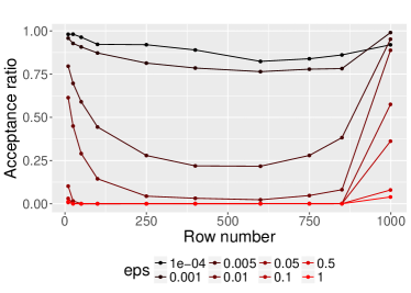
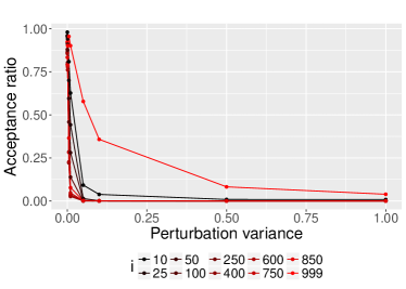
Figure 1: Acceptance ratio as a function of the row number $i$ (left) and the perturbation variance $\sigma_{\epsilon}^{2}$ (right). eps: $\sigma_{\epsilon}^{2}$.

We observe how, as $\sigma_{\epsilon}^{2}$ increases, the proposed value is rejected more often. This could be already expected by looking at Equation (5) above, where we see that the second term goes to zero as $\sigma_{\epsilon}^{2}$ increases, yielding $\lim_{\sigma_{\epsilon}^{2}\to\infty}P(f(\boldsymbol{v})\leq f(\tilde{\boldsymbol{v}}))\leq 1/2$. Furthermore, as $\sigma_{\epsilon}$ increases the proposal distribution is more similar to the uniform density on the $(p-i)$-dimensional sphere (Equation (6)), which also hints the higher rejection rate.

The row number $i$ also has a significant influence on the acceptance ratio. Recall that $1\leq i\leq p-1$, $\boldsymbol{v}\in\mathcal{S}^{p-i}_{+}$ and $f(\boldsymbol{v})\propto v_{1}^{i}$, therefore as the row number $i$ increases the target distribution $f$ approaches a delta function, and the dimensionality of $\boldsymbol{v}$ decreases. Therefore it is reasonable to assume that the larger $i$ is, the smaller $\sigma_{\epsilon}^{2}$ should be for achieving a high acceptance ratio, since it means that we are proposing new states that are, with high probability, very close to the current state.

The above conclusions are further illustrated in Figure 2, where we have plotted the contour lines of the acceptance ratio surface as a function of $\sigma_{\epsilon}^{2}$ and the row number $i$. Observe that small values for $\sigma_{\epsilon}$ always lead to high acceptance ratios, however this might not always be desirable since it can be a sign of slow convergence. By contrast, a low acceptance ratio can be expected when approaching to a delta in moderately high dimensions, as is the case for row numbers approximately between $250$ and $750$.

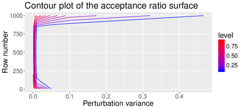
Figure 2: Contour lines of the acceptance ratio surface. level: magnitude of the acceptance ratio.

5 Performance analysis

In this section we will compare our method, in terms of computational performance, with the existing approaches in the literature for the same task: uniform sampling of correlation matrices. We will generate $5000$ correlation matrices of dimension $p=10,20,\ldots,100$ using our algorithm, the vine and onion methods of Lewandowski et al. [6], and the polar parametrization of Pourahmadi [9].

Our algorithm has been implemented in R [11]. The vine and onion methods are available in the function genPositiveDefMat from the R package clusterGeneration, provided by the authors. Since we have not found an implementation of the polar parametrization method of Pourahmadi [9], we have developed our own function, also in R, mimicking the method therein described. For our method, based on the analysis of the previous section we have fixed $\sigma_{\epsilon}=0.01$ and $t_{b}=1000$, which have empirically provided good convergence results. The experiment has been executed on a machine equipped with Intel Core i7-5820k, $3.30$ GHz$\times 12$ and $16$ GB of RAM.

The results of the experiment are shown in Figure 3. We observe that our method is faster than all of the existing approaches in the literature. The polar parametrization method has the worst performance, several orders of magnitude slower than the other algorithms. This can be explained by the use of inverse transformation sampling for simulating the angles. By contrast, our method achieves highly competitive results by taking advantage of the direct representation provided by the Cholesky factorization, as well as the simple form of the target distribution and the proposed values on each iteration. The scripts used for generating the data and figures described throughout the paper are publicly available, as well as the implementation of the algorithms described, so all the above experiments can be replicated.

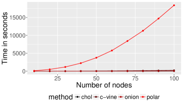
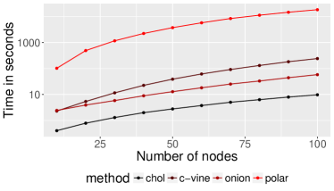
Figure 3: Execution time of available methods for uniform sampling of correlation matrices, both in linear (left) and logarithmic (right) scale. chol: our proposal; c-vine, onion: methods by [6]; polar: method by [9].

6 Conclusions

In this paper we have proposed a Metropolis-Hastings method for uniform sampling of correlation matrices. We have studied its properties, both theoretically and empirically, and shown fast convergence to the target uniform distribution. We have also executed a comparative performance study, where our approach has yielded faster results than all of the related approaches in the literature.

In the future, we would like to further explore variants of our Markov chain algorithm, such as the independent Metropolis or adaptive schemes. We would also like to expand on the theoretical convergence analysis of such variants, as well extend the empirical convergence monitoring to other relevant quantities apart from the acceptance ratio.

Acknowledgements. This work has been partially supported by the Spanish Ministry of Economy, Industry and Competitiveness through the Cajal Blue Brain (C080020-09; the Spanish partner of the EPFL Blue Brain initiative) and TIN2016-79684-P projects; by the Regional Government of Madrid through the S2013/ICE-2845-CASI-CAM-CM project; and by Fundación BBVA grants to Scientific Research Teams in Big Data 2016. I. Córdoba has been supported by the predoctoral grant FPU15/03797 from the Spanish Ministry of Education, Culture and Sports. G. Varando has been partially supported by research grant 13358 from VILLUM FONDEN.

References

- [1] Diaconis, P., Holmes, S., Shahshahani, M.: Sampling from a Manifold, Collections, vol. 10, pp. 102–125. Institute of Mathematical Statistics (2013)
- [2] Eaton, M.L.: Multivariate Statistics: A Vector Space Approach. Wiley (1983)
- [3] Fallat, S., Lauritzen, S., Sadeghi, K., Uhler, C., Wermuth, N., Zwiernik, P.: Total positivity in markov structures. The Annals of Statistics 45(3), 1152–1184 (2017)
- [4] Holmes, R.: On random correlation matrices. SIAM Journal on Matrix Analysis and Applications 12(2), 239–272 (1991)
- [5] Laurent, M., Poljak, S.: On the facial structure of the set of correlation matrices. SIAM Journal on Matrix Analysis and Applications 17(3), 530–547 (1996)
- [6] Lewandowski, D., Kurowicka, D., Joe, H.: Generating random correlation matrices based on vines and extended onion method. Journal of Multivariate Analysis 100(9), 1989–2001 (2009)
- [7] Mardia, K., Jupp, P.: Directional Statistics. Wiley (1999)
- [8] Marsaglia, G., Olkin, I.: Generating correlation matrices. SIAM Journal on Scientific and Statistical Computing 5(2), 470–475 (1984)
- [9] Pourahmadi, M., Wang, X.: Distribution of random correlation matrices: Hyperspherical parameterization of the Cholesky factor. Statistics & Probability Letters 106, 5–12 (2015)
- [10] Pukkila, T.M., Rao, C.R.: Pattern recognition based on scale invariant discriminant functions. Information Sciences 45(3), 379–389 (1988)
- [11] R Core Team: R: A Language and Environment for Statistical Computing. R Foundation for Statistical Computing, Vienna, Austria (2018)
- [12] Robert, C., Casella, G.: Monte Carlo Statistical Methods. Springer (2004)