Dynamic Modulation Yields One-Way Beam Splitting

Abstract

This article demonstrates the realization of an extraordinary beam splitter, exhibiting one-way beam splitting-amplification. Such a dynamic beam splitter operates based on nonreciprocal and synchronized photonic transitions in obliquely illuminated space-time-modulated (STM) slabs which impart the coherent temporal frequency and spatial frequency shifts. As a consequence of such unusual photonic transitions, a is exhibited by the STM slab. Beam splitting is a vital operation for various communication systems, including circuit quantum electrodynamics, and signal-multiplexing and demultiplexhg. Despite the beam splitting is conceptually a simple operation, the performance characteristics of beam splitters significantly influence the repeatability and accuracy of the entire system. As of today, there has been no approach exhibiting a nonreciprocal beam splitting accompanied with transmission gain and an arbitrary splitting angle. Here, we show that oblique illumination of a periodic and semi-coherent dynamically-modulated slab results in coherent photonic transitions between the incident light beam and its counterpart space-time harmonic (STH). Such transitions introduce a unidirectional synchronization and momentum exchange between two STHs with same temporal frequencies, but opposite spatial frequencies. Such a beam splitting technique offers high isolation, transmission gain and zero beam tilting, and is expected to drastically decrease the resource and isolation requirements in communication systems. In addition to the analytical solution, we provide a closed-form solution for the electromagnetic fields in STM structures, and accordingly, investigate the properties of the wave isolation and amplification in subluminal, superluminal and luminal ST modulations.

I Introduction

Beam splitters are quintessential elements of communication systems Schneider (2014); Hammer et al. (2015); Tan and Yassin (2017); Watanabe (1980); Zhu et al. (2006); Hwang et al. (2012); Cooper et al. (2012); Watanabe (1980). In the microwave regime, beam splitters are required for the generation of single photons in the circuit quantum electrodynamics Wallraff et al. (2004); Blais et al. (2004); Mariantoni et al. (2008); Schneider (2014); Houck et al. (2007); Bozyigit et al. (2011a, b), heterodyne mixer arrays Tan and Yassin (2017), and wave engineering and signal-multiplexing and demultiplexhg Watanabe (1980); Zhu et al. (2006); Hwang et al. (2012); Cooper et al. (2012); Watanabe (1980). However, the realization of microwave on-chip beam splitters is still under research and development Mariantoni et al. (2010); Schneider (2014); Hammer et al. (2015). In spite of the immense scientific attempts for the realization of efficient beam splitters, beam splitters are restricted to reciprocal response and suffer from substantial transmission loss. As a consequence, the resource requirements of the overall system, including demand for high power microwave sources and isolators, will be increased.

This paper presents the application of space-time-modulated (STM) structures to extraordinary beam splitting. As of today, various applications of STM structures have been reported, where normal incidence of the light beam to the STM structure yields unusual interaction with electromagnetic wave Cassedy (1967); Yu and Fan (2009); Taravati (2018a); Taravati et al. (2017); Salary et al. (2018a, b); Taravati and Kishk (2019). These applications include but not limited to the parametric traveling-wave amplifiers Cullen (1958); Tien (1958); Tien and Suhl (1958); Cassedy and Oliner (1963), isolators Wentz (1966); Bhandare et al. (2005); Lira et al. (2012); Taravati et al. (2017); Chamanara et al. (2017); Taravati (2017); Kim et al. (2017); Sohn et al. (2018), metasurfaces Hadad et al. (2015); Shi and Fan (2016); Shi et al. (2017); Wu and Grbic (2018), pure frequency mixer Taravati (2018b), circulators Qin et al. (2014); Estep et al. (2014); Reiskarimian et al. (2018), and mixer-duplexer-antenna system Taravati and Caloz (2015, 2017). Nevertheless, there has been a lack of investigation on the properties of STM media under oblique incidence and its applications.

Here, we introduce a one-way, tunable and highly efficient beam splitter and amplifier based on coherent photonic transitions through the oblique illumination of STM structures. The contributions of this paper are as follows.

1) In contrast to conventional beam splitters which are restricted to reciprocal response with more than 3 dB insertion loss, the proposed STM beam splitter is capable of providing nonreciprocal response with transmission gain. It can be also used in antenna applications, where the transmitted and received waves are engineered appropriately.

2) We show that the STM beam splitter presents an efficient performance for both collimated and non-collimated incidence beam with no output beam tilt. This is very interesting as conventional passive beam splitters suffer from poor performance for non-collimated beams and provide an undesired output beam tilt.

3) It is demonstrated that the angle of transmission and the amplitude of the transmitted beams depend on the ST modulation parameters. Hence, the ST modulation parameters provide the leverage for achieving the desired angle of transmission for the two output beams of the STM beam splitter. In addition, unequal power division between the output beams can be achieved by varying the ST modulation parameters.

4) Here, we present the first application of obliquely illuminated STM slabs. Consequently, for the first time, the scheme and results for the finite difference time-domain (FDTD) simulation results for oblique incidence to a STM slab at microwave frequencies is presented.

5) A closed-form solution is presented that provides a deep insight into the wave propagation inside the STM beam splitters and the difference between the subluminal, luminal and superluminal ST modulations.

6) The analysis of the STM beam splitter is further accomplished by investigation of its analytical three dimensional dispersion diagrams, achieved by Bloch-Floquet decomposition of space-time harmonics (STHs).

Accordingly, the rest of the paper is structured as follows. Section II presents the operation principle of the proposed STM beam splitter. In Sec. III, we derive the analytical solution for oblique electromagnetic wave propagation inside the STM beam splitter based on the Bloch-Floquet representation of the electromagnetic fields. Then, Sec. IV presents the time and frequency domains numerical simulation results for the beam splitting and amplification in the STM beam splitter. Next, the closed form solution will be provided in Sec. V, which gives a leverage for understanding the wave propagation and transitions in STM structures. A short discussion on practical realization of superluminal STM structures at different frequencies will be presented in Sec. VI. Finally, Sec. VII concludes the paper.

II Operation Principle

Figure 1 sketches the nonreciprocal beam transmission and splitting in a STM slab. By appropriate design of the band structure, that is, the ST modulation format and its associated temporal and spatial modulation frequencies, unidirectional energy and momentum exchange between the incident wave-under angle of incidence and transmission $\theta_{\text{I}}=\theta_{\text{T},0}=45^{\circ}$ and temporal frequency $\omega_{0}$- to the first lower STH-under angle of transmission $\theta_{\text{T},-1}=-45^{\circ}$ and temporal frequency $\omega_{0}$- will occur. Assuming $\text{TM}_{y}$ or $E_{y}$ polarization, the electric field of the incident light beam in the forward $+z$-direction may be expressed as

$$E_{\text{I}}^{\text{F}}(x,z,t)=E_{0}e^{-i\left[k_{x}x+k_{z}z-\omega_{0}t\right]},$$ (1)

is traveling in the $+z$-direction under the angle of incidence $\theta_{\text{I}}=45^{\circ}$ and impinges to the periodic STM slab. The $x$- and $z$-components of the spatial frequency read $k_{x}=k_{0}\sin(\theta_{\text{I}})$ and $k_{z}=k_{0}\cos(\theta_{\text{I}})$, respectively, in which $k_{0}=\omega_{0}/v_{\text{b}}=\omega_{0}\sqrt{\epsilon_{\text{r}}}/c$, with $\omega_{0}$ being the temporal frequency of the incident wave, $v_{\text{b}}$ denoting the phase velocity in the background medium, $\epsilon_{\text{r}}$ representing the relative electric permittivity of the background medium, and $c$ denoting the speed of light in vacuum.

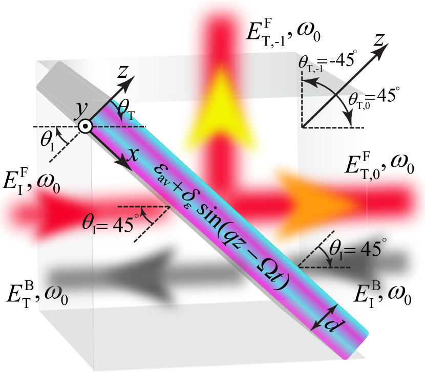
Figure 1: Schematic of nonreciprocal beam splitting in a STM slab. The slab varies in time two times faster than the input wave.

The STM slab assumes a sinusoidal ST-varying permittivity, as

$$\epsilon(z,t)=\epsilon_{\text{av}}+\delta_{\epsilon}\sin(qz-\Omega t),$$ (2)

where $\epsilon_{\text{av}}=\epsilon_{\text{r}}+\delta_{\epsilon}$ is the average permittivity of the slab, $\delta_{\epsilon}$ denotes the modulation strength, $\Omega=2\omega_{0}$ is the modulation temporal frequency, and

$$q=\frac{2k_{0}}{\gamma},$$ (3)

represents the spatial frequency of the modulation, with $\gamma=v_{\text{m}}/v_{\text{b}}$ being the ST velocity ratio, where $v_{\text{m}}$ and $v_{\text{b}}$ are, the phase velocity of the modulation and the background medium, respectively. Since the slab permittivity is periodic in space and time, with spatial frequency $q$ and temporal frequency $2\omega_{0}$, the electric field inside the slab may be decomposed into ST Bloch-Floquet waves as

$$\mathbf{E}_{\text{S}}(x,z,t)=\mathbf{\hat{y}}\sum_{m=-M}^{M}A_{m}e^{-i\left(k_{x}x+k_{z,m}z-\omega_{m}t\right)},$$ (4a)

and

$$\begin{split}&\mathbf{H}_{\text{S}}(x,z,t)=\frac{1}{\eta_{\text{S}}}\left[\mathbf{\hat{k}}_{\text{S}}\times\mathbf{E}_{\text{S}}(x,z,t)\right]\\ &=\sum_{m=-M}^{M}\bigg{[}-\mathbf{\hat{x}}\frac{k_{z,m}}{\mu_{0}\omega_{m}}+\mathbf{\hat{z}}\frac{\sin(\theta_{\text{I}})}{\eta_{\text{S}}}\bigg{]}A_{m}e^{-i\left(k_{x}x+k_{z,m}z-\omega_{m}t\right)}.\end{split}$$ (4b)

where $$M\rightarrow\infty \eta_{\text{S}}=\sqrt{\mu_{0}/(\epsilon_{0}\epsilon_{r})} A_{m} m$$ is the number of STHs. In Eq. (4), , and represents the unknown amplitude of the th STH, characterized by the spatial frequency

$$k_{z,m}=\beta_{0}+mq,$$ (4c)

and the temporal frequency

$$\omega_{m}=\omega_{0}+m\Omega=(1+2m)\omega_{0},$$ (4d)

with $\beta_{0}$ being the unknown spatial frequency of the fundamental harmonic. The unknowns of the electric field, that is, $A_{m}$ and $\beta_{0}$, will be found through satisfying Maxwell’s equations.

The transmission angle of the $m$th transmitted STH, $\theta_{\text{T},m}$, satisfies the Helmholtz relation as

$$k_{0}^{2}\sin^{2}(\theta_{\text{I}})+k_{m}^{2}\cos^{2}(\theta_{\text{T},m})=k_{m}^{2},$$ (5)

where $k_{m}=\omega_{m}/v_{\text{b}}$ denotes the wavenumber of the $m$th transmitted STH outside the STM slab. Solving Eq. (5) for $\theta_{\text{T},m}$ yields

$$\begin{split}\theta_{\text{T},m}=\sin^{-1}\left(\frac{k_{x}}{k_{m}}\right)&=\sin^{-1}\left(\frac{\sin(\theta_{\text{I}})}{1+m\Omega/\omega_{0}}\right)\\ &=\sin^{-1}\left(\frac{\sin(\theta_{\text{I}})}{1+2m}\right).\end{split}$$ (6a)

Equation (6a) demonstrates the spectral decomposition of the transmitted wave. Consequently, the fundamental STH, $m=0$, and the first lower STH, $m=-1$, with equal temporal frequency $\omega_{0}$, will be respectively transmitted under the angles of transmission of

$$\begin{split}\theta_{\text{T},0}&=\theta_{\text{I}}=45^{\circ},\\ \theta_{\text{T},-1}&=-\theta_{\text{I}}=-45^{\circ}.\end{split}$$ (6b)

so that they are transmitted under $90^{\circ}$ angle difference, presenting the desired beam splitting. The scattering angle of the $m$th STH inside the STM slab reads

$$\theta_{\text{S},m}=\tan^{-1}\left(\frac{k_{x}}{k_{z,m}}\right).$$ (7)

In addition, the transmitted electric field from the slab may be found as

$$\begin{split}\mathbf{E}_{\text{T}}(x,z,t)&=\mathbf{E}_{\text{S}}(x,z,t)e^{-ik_{z,m}z}\\ &=\mathbf{\hat{y}}\sum_{m=-M}^{M}A_{m}e^{-i\left(k_{x}x+k_{z,m}[d+z]-\omega_{m}t\right)}.\end{split}$$ (8)

The sourceless wave equation reads

$$\nabla^{2}\mathbf{E}_{\text{S}}(x,z,t)-\frac{1}{{{c^{2}}}}\frac{{{\partial^{2}}\left[\epsilon(z,t)\mathbf{E}_{\text{S}}(x,z,t)\right]}}{{\partial{t^{2}}}}=0.$$ (9)

Substituting Eqs. (S1) and (4) into Maxwell’s equations, yields a matrix equation as

$$[K]\vec{A}=0,$$ (10a)

where $$[K] (2M+1)\times(2M+1)$$ is a matrix with elements

$$\begin{split}&K_{m,m}=\epsilon_{\text{av}}-\frac{k_{x}^{2}+k_{z,m}^{2}}{k_{0}^{2}},\\ &K_{m,m-1}=i\frac{\delta_{\epsilon}}{2},\\ &K_{m,m+1}=-i\frac{\delta_{\epsilon}}{2},\end{split}$$ (10b)

and where $\vec{A}$ represents a $(2M+1)\times 1$ vector containing $A_{m}$ coefficients. Equation (10a) has nontrivial solution if

$$\text{det}\left\{[K]\right\}=0.$$ (11)

Equation (11) represents the dispersion relation of the STM beam splitter which provides the unknown spatial frequency of the fundamental ST harmonic for a given frequency, i.e., $\beta_{0}(\omega_{0})$. After finding the $\beta_{0}(\omega_{0})$, the $[K]$ matrix in Eq. (10a) is known and therefor, the unknown amplitude of the STHs $A_{m}$ will be calculated using Eq. (10a).

III Analytical 3D Dispersion Diagram

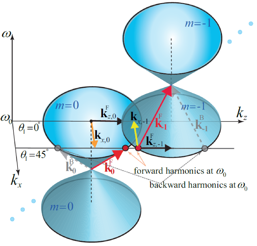
Figure 2: Qualitative representation of the periodic three dimensional dispersion diagram for the periodic STM slab in Fig. 1. The medium is under oblique illumination of $\theta_{\text{I}}=45^{\circ}$ at the fundamental harmonic $m=0$, corresponding to the temporal frequency $\omega_{0}$, where $\textbf{k}_{x,0}=\mathbf{\hat{x}}k_{x}=\mathbf{\hat{x}}k_{0}\sin(\theta_{\text{I}})$. The lower STH, $m=-1$, provides the same temporal frequency as the fundamental harmonic, $|\omega_{m}|=|\omega_{0}(1+2m)|_{m=-1}=\omega_{0}$, but opposite $x$-component of the spatial frequency, that is, $\textbf{k}_{x,-1}=-\mathbf{\hat{x}}k_{x}=-\mathbf{\hat{x}}k_{0}\sin(\theta_{\text{I}})$.

Figure 2 presents a qualitative illustration of the three dimensional dispersion diagram in the STM medium in Fig. 1 achieved using Eq. (11). This diagram is formed by $2M+1$ periodic set of double cones (here, only $m=0$ and $m=-1$ harmonics are shown), each of which representing a STH, with apexes at $k_{x}=0$, $k_{z}=-mq$ and $\omega=-2m\omega_{0}$, and the slope of $v_{m}$ with respect to $k_{z}-k_{x}$ plane. Consider oblique incidence of a wave, representing the fundamental harmonic $m=0$ with temporal frequency $\omega_{0}$, propagating along [$+x$,$+z$] direction. It is characterized by $x$- and $z$-components of the spatial frequency, $\textbf{k}_{x}=\mathbf{\hat{x}}k_{x}$ and $\textbf{k}_{z}^{\text{F}}=\mathbf{\hat{z}}k_{z}$. The wave impinges to the medium under the angle of incidence $\theta_{\text{I}}=45^{\circ}$ and excites an infinite number of (we truncate it to $2M+1$) STH waves, with different spatial and temporal frequencies of $[k_{x},k_{z,m}]$ and $\omega_{m}$. However, interestingly, the first lower STH $m=-1$ offers similar characteristics as the fundamental harmonic, that is, the identical temporal frequency of $\omega_{0}$ and identical $z$-component of the spatial frequency of $\textbf{k}_{z,-1}^{\text{F}}=\textbf{k}_{z,0}^{\text{F}}$, but opposite $x$-component of the spatial frequency of $\textbf{k}_{x,-1}=-\textbf{k}_{x,0}$. Hence, $m=-1$ harmonic propagates along [$-x$,$+z$] direction. In general the $x$-component of the $m$th STH reads $\textbf{k}_{x,m}=-\textbf{k}_{x,-m-1}$). Moreover, since $\omega_{m}=\omega_{-m-1}$, the undesired STHs acquire temporal frequency of $2m\omega_{0}$, and far away from the fundamental harmonic. Thus, most of the incident energy is residing in $m=0$ and $m=-1$ harmonics, both at $\omega_{0}$, respectively transmitted under $\theta_{\text{T,0}}=\theta_{\text{I}}$ and $\theta_{\text{T,-1}}=-\theta_{\text{I}}$ transmission angles with $2\theta_{\text{I}}$ angle difference.

The exchange of the energy and momentum between the fundamental and first lower harmonic occurs only for the forward, $+z$, wave incidence. This may be observed from Fig. 2, as the forward harmonics (red circles, where $\partial\omega/\partial k_{z}>0$) are very close, whereas the backward harmonics (grey circles, where $\partial\omega/\partial k_{z}<0$) are far apart from each other. Therefore, a nonreciprocal transition of energy is achieved from the incident wave under $\theta_{\text{I}}=45^{\circ}$ to the first STH under $\theta_{\text{T,-1}}=-45^{\circ}$, through the ST modulation under $\theta_{\text{mod}}=0^{\circ}$.

Figure 3 shows the analytical solution for three dimensional dispersion diagram of the STM medium in Fig. 1, computed using Eq. (11) for $\gamma=1.2$. For a given frequency, this three dimensional diagram provides the two dimensional $k_{z}/q-k_{x}/q$ isofrequency diagram of the medium. Figure 3 plots the isofrequency diagram at $\omega/2\omega_{0}=0.5$ (or $\omega=\omega_{0}$), containing an infinite periodic set of circles centered at $(k_{z}/q,k_{x}/q)=(-m,0)$ with radius $\gamma(0.5+m)$.

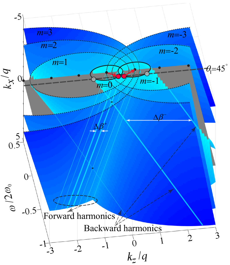
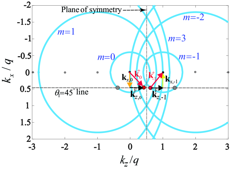
Figure 3: Analytical dispersion diagram of the periodic STM slab in Fig. 1 for $\gamma=1.2$ computed using Eq. (11). The forward incidence under $\theta_{\text{I}}=45^{\circ}$ corresponding to $k_{x}/q=0.4243$ excites the $m=-1$ STH, resulting in a strong exchange of energy between $m=0$ and $m=-1$ harmonics, with the identical temporal frequency of $\Omega_{0}$. (a) Three dimensional dispersion diagram constituted of an array of periodic cones Taravati et al. (2017). (b) Isofrequency diagram at $\omega=\omega_{0}$ presents an infinite set of circles centered at $(k_{z}/q,k_{x}/q)=(-m,0)$ with radius $\gamma(0.5+m)$.

It may be seen from Figs. 3 and 3 that at $\omega=\omega_{0}$, the $m=0$ and $m=-1$ STHs offer identical isofrequency circles. However, their associated forward harmonics (red circles) are very close to each other whereas their associated backward harmonics (grey circles) are significantly separated. For a nonzero velocity ratio ($\gamma>0$), the forward and backward STHs acquire different distances, i.e. $\Delta\beta^{\pm}=k_{z,m+1}^{\pm}-k_{z,m}^{\pm}$ Taravati et al. (2017). Particularly, as $\gamma$ increases, $\Delta\beta^{-}$ increases and $\Delta\beta^{+}$ decreases. As a result, at the limit of $\gamma=1$ the forward harmonics acquire distances $\Delta\beta^{+}/q=0$, and the backward harmonics acquire distances $\Delta\beta^{-}/q=2$. Hence, increasing $\gamma$ results in the significant enhancement in the nonreciprocity of the medium, so that the forward harmonic waves tend to merge together ($\Delta\beta^{+}\rightarrow 0$) and exchange their energy and momentum, whereas the backward harmonics tend to separate from each other ($\Delta\beta^{+}\rightarrow 2$) (Fig. 3). Hence, such a dynamic modulation has nearly no effect on the backward incident beam.

IV Numerical Simulation Results

We next verify the above theory by finite difference time-domain (FDTD) numerical simulation of the dynamic process through solving Maxwell’s equations. Figure 4 plots the implemented finite-difference time-domain scheme for numerical simulation of the oblique wave impinging to the STM beam splitter. We first discretize the medium to $K+1$ spatial samples and $M+1$ temporal samples, with the steps of $\Delta z$ and $\Delta t$, respectively.

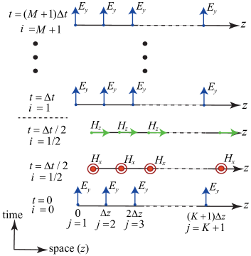
Figure 4: General representation of the finite-difference time-domain scheme for numerical simulation of the oblique incidence of an $E_{y}$ wave to STM beam splitter.

Next, the finite-difference discretized form of the first two Maxwell’s equations for the electric and magnetic fields (considering Eq. (4)) will be simplified to

$$\begin{split}H_{x}\lvert_{j+1/2}^{i+1/2}=&\left(1-\Delta t\right)H_{x}\lvert_{j+1/2}^{i-1/2}+\dfrac{\Delta t}{\mu_{0}\Delta z}\left(E_{y}\lvert_{j+1}^{i}-E_{y}\lvert_{j}^{i}\right)\end{split}$$ (12a)

$$\begin{split}H_{z}\lvert_{j+1/2}^{i+1/2}=&\left(1-\Delta t\right)H_{z}\lvert_{j+1/2}^{i-1/2}-\dfrac{\Delta t}{\mu_{0}\Delta z}\left(E_{y}\lvert_{j+1}^{i}-E_{y}\lvert_{j}^{i}\right)\end{split}$$ (12b)

$$\begin{split}E_{y}&\lvert_{j}^{i+1}=\left(1-\dfrac{\Delta t\epsilon^{\prime}\lvert_{j}^{i}}{\epsilon\lvert_{j}^{i+1/2}}\right)E_{y}\lvert_{j}^{i}+\dfrac{\Delta t/\Delta z}{\epsilon\lvert_{j}^{i+1/2}}\\ &.\left[\left(H_{x}\lvert_{j+1/2}^{i+1/2}-H_{x}\lvert_{j-1/2}^{i+1/2}\right)-\left(H_{z}\lvert_{j+1/2}^{i+1/2}-H_{z}\lvert_{j-1/2}^{i+1/2}\right)\right]\end{split}$$ (12c)

where $\epsilon^{\prime}=\partial\epsilon(z,t)/\partial t=-\Omega\delta_{\epsilon}\cos(qz-\Omega t)$.

Figure 5 shows the numerical simulation results for the forward oblique wave incidence to the slab, shown in Fig. 1, with $\epsilon_{\text{r}}=1$, $\delta_{\epsilon}=0.2$, $\gamma=1.2$, $d=3\lambda_{0}=3\times 2\pi/k_{0}$, $\theta_{\text{I}}=45^{\circ}$ and $\omega_{\text{0}}=3$ GHz. It may be seen from this figure that an efficient beam splitting with significant transmission gain is achieved in the forward direction. Figures 6 and 6 provide the results for the oblique wave incidence from the right side and top, respectively, corresponding to $\theta_{\text{I}}=45^{\circ}$ and $\theta_{\text{I}}=-45^{\circ}$. The presented analytical and numerical results demonstrate that the dynamic beam splitter provides a perfect nonreciprocal beam splitting, in the lack of beam tilting. Moreover, it may be seen that, in contrast to conventional passive beam splitters, the beam splitting is achieved for a non-collimated beam. Other interesting features may be presented by changing the modulation parameters ($\gamma$, $\theta_{\text{I}}$ and $\epsilon_{\text{av}}$), including tunable transmission angles, unequal splitting ratio and unequal angles of transmission. Figure 7 compares the analytical and numerical results for the spectrum of the incident and transmitted electric fields in Fig. 5. This figure shows that $3$dB transmission gain is achieved for each of transmitted beams in the forward excitation. Moreover, it may be seen from Fig. 7 that the undesired higher order harmonics, at $\omega=2m\omega_{0}$, are sufficiently weak so that the beam splitter safely operates at single frequency $\omega_{0}$.

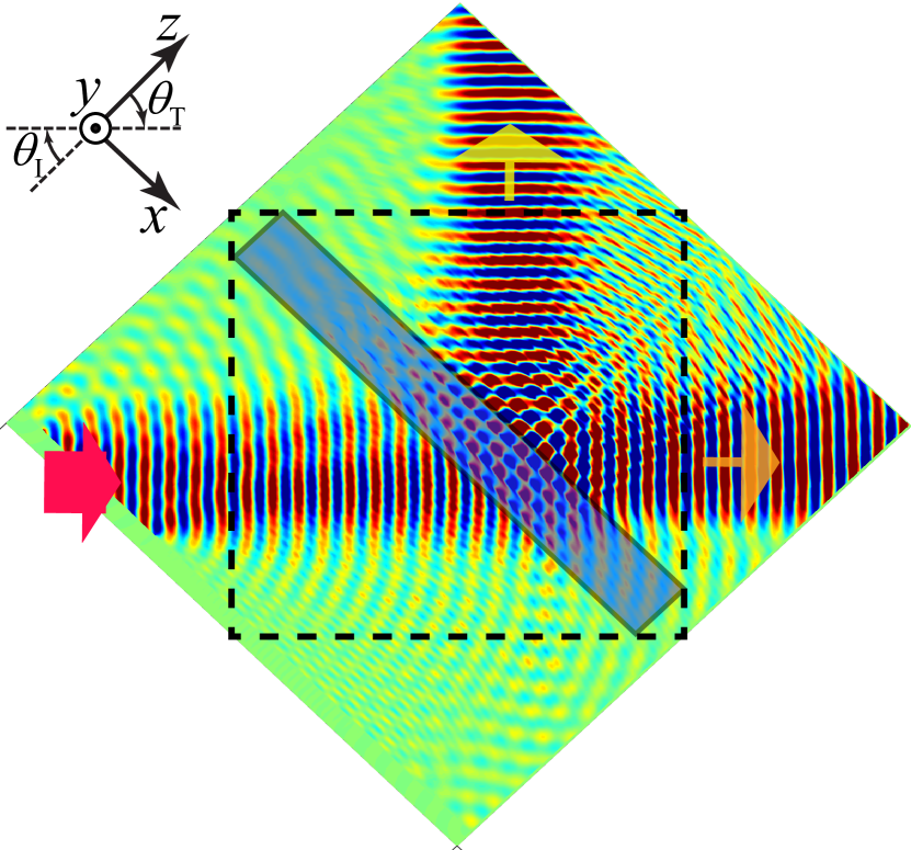
Figure 5: Nonreciprocal beam splitting in periodically STM slab. FDTD numerical simulation for the forward wave incidence to the slab, from the left, with $\theta_{\text{I}}=45^{\circ}$.

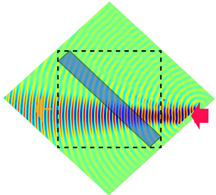
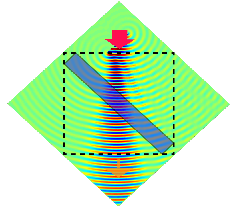
Figure 6: Nonreciprocal beam splitting in periodically STM slab. FDTD numerical simulation for the wave incidence to the slab, (a) From the right with $\theta_{\text{I}}=45^{\circ}$. (b) From the top, i.e., $\theta_{\text{I}}=-45^{\circ}$.

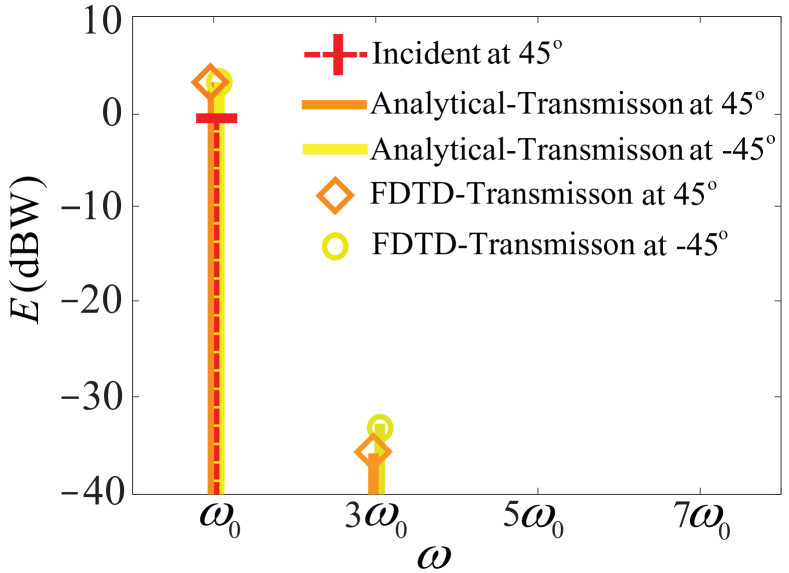
Figure 7: Comparison of the analytical and numerical results for the frequency spectrum of the incident and transmitted electric fields in Fig. 5, i.e., wave incidence to the slab from the left with $\theta_{\text{I}}=45^{\circ}$.

V Closed form Solution for Electromagnetic Fields

It is shown in Sec. IV that by proper design of the band structure, a pure unidirectional beam splitting can be achieved in a obliquely illuminated STM slab. The analytical solution of the electromagnetic fields based on the double Bloch-Floquet decomposition of electromagnetic fields, presented in Sec. III, provides an accurate solution for the fields scattered by such a slab, which is very useful. However, such an analytical solution does not provide a deep insight into the wave propagation inside the slab. In particular, it is of great interest to have an intuitive explanation about the effect of different parameters, e.g. $\delta_{\epsilon}$, $\gamma$, $k_{x}$ and $k_{z}$, on the wave propagation and energy exchange between the incident field $m=0$ and the excited first lower harmonic $m=-1$. Moreover, the accurate analytical solution, based on the mathematical modeling presented in Sec. III, is achieved through a substantial computational cost. To resolve this issue, here we provide an approximate closed form solution for the electromagnetic fields propagating inside and transmitted from the STM beam splitter, which provides a clear picture of the transition between the incident and the first lower STHs.

As we showed in the previous section, given the weak transition of energy and momentum from the fundamental STH $m=0$ to higher order STHS except $m=-1$, the electric field inside the STM slab may be represented based on the superposition of the aforementioned two STHs, i.e., $m=0$ and $m=-1$. The electric field is then defined by

$$\begin{split}E_{\text{S}}(x,z,t)=&a_{0}(z)e^{-i\left(k_{x}x+k_{z}z-\omega_{0}t\right)}\\ &+a_{-1}(z)e^{i\left(-k_{x}x+(q-k_{z})z-\omega_{0}t\right)},\end{split}$$ (13)

where $a_{0}(z)$ and $a_{-1}(z)$ are the unknown field coefficients. We shall stress that, here the field coefficients are $z$-dependent since they include both the amplitude and the change in the spatial frequency (wavenumber) introduced by the ST modulation. Following the procedure provided in the supplemental material in Ref. Tar , we insert the electric fields in (13) into the wave equations in (S4), and achieve a coupled differential equation for the field coefficients, i.e.,

$$\frac{d}{dz}\begin{bmatrix}a_{0}(z)\\ a_{-1}(z)\end{bmatrix}=\begin{bmatrix}M_{0}&C_{0}\\ C_{-1}&M_{-1}\end{bmatrix}\begin{bmatrix}a_{0}(z)\\ a_{-1}(z)\end{bmatrix},$$ (14a)

where

$$M_{0} =\frac{ik_{0}^{2}}{2k_{z}}(\epsilon_{\text{av}}-\epsilon_{\text{r}}),$$

$$M_{-1} =\frac{ik_{0}^{2}}{2(k_{z}-q)}\left[\epsilon_{\text{av}}-\epsilon_{\text{r}}\frac{k_{x}^{2}+(q-k_{z})^{2}}{k_{0}^{2}}\right],$$

$$C_{0} =i\frac{\delta k_{0}^{2}}{4k_{z}},$$

$$C_{-1} =i\frac{\delta k_{0}^{2}}{4(k_{z}-q)}.$$ (14b)

The solution to the coupled differential equation in (14a) is given by Tar

$$a_{0}(z)=\frac{E_{0}}{2\varDelta} \bigg{(}(M_{0}-M_{-1}+\varDelta)e^{\frac{M_{0}+M_{-1}+\varDelta}{2}z}$$ (15a)

$$-(M_{0}-M_{-1}-\varDelta)e^{\frac{M_{0}+M_{-1}-\varDelta}{2}z}\bigg{)},$$

$$a_{-1}(z)=\frac{E_{0}C_{-1}}{\varDelta}\left(e^{\frac{M_{0}+M_{-1}+\varDelta}{2}z}-e^{\frac{M_{0}+M_{-1}-\varDelta}{2}z}\right),$$ (15b)

where $\varDelta=\sqrt{(M_{0}-M_{-1})^{2}+4C_{0}C_{-1}}$. For a given ST modulation ratio $\gamma$, the field coefficients in Eq. (15) acquire different forms. In general, ST modulation is classified into three categories, i.e., subluminal ($0<\gamma<1$ or $v_{\text{m}}<v_{\text{b}}$), luminal ($\gamma\rightarrow 1$ or $v_{\text{m}}\rightarrow v_{\text{b}}$), and superluminal ($\gamma>1$ or $v_{\text{m}}>v_{\text{b}}$).

V.1 Subluminal and Superluminal ST Modulations

Considering $\epsilon_{\text{av}}=\epsilon_{\text{r}}$, the $a_{0}(z)$ and $a_{-1}(z)$ in Eq. (15) would be a periodic sinusoidal function with respect to $z$, if $\varDelta=\sqrt{(M_{0}-M_{-1})^{2}+4C_{0}C_{-1}}$ is imaginary, i.e., $(M_{0}-M_{-1})^{2}+4C_{0}C_{-1}<0$. By solving this, we achieve an interval for the luminal ST modulation, that is,

$$\gamma_{\text{sub}}<\frac{1}{\sqrt{\epsilon_{\text{av}}+\delta_{\epsilon}}}\leq\gamma_{\text{lum}}\leq\frac{1}{\sqrt{\epsilon_{\text{av}}-\delta_{\epsilon}}}<\gamma_{\text{sup}},$$ (16)

where $\gamma_{\text{sub}}$, $\gamma_{\text{lum}}$ and $\gamma_{\text{sup}}$ are ST velocity ratio for subluminal, luminal and superluminal ST modulations, respectively. The interval for luminal ST modulation is called sonic regime in analogy with sonic boom effect in acoustics, where an airplane travels with the same speed or faster than the speed of sound. It should be noted that the luminal ST modulation interval in Eq. (16) is exactly same as the one achieved from the exact analytical solution Cassedy and Oliner (1963); Taravati et al. (2017); Taravati (2018a).

Figure 8 plots the closed form and FDTD numerical simulation results for the absolute electric field coefficient inside the slab, with the wave incidence from the left side (forward incidence), considering superluminal ST modulation of $\gamma=1.2$ and $\delta_{\epsilon}=0.28$. It is seen from this figure that both $a_{0}(z)$ and $a_{-1}(z)$ possess periodic sinusoidal form and exhibit a substantial transmission gain at $z=3\lambda_{0}$. Such a transmission gain may be tuned through the variation of $\gamma$ and $\delta_{\epsilon}$. This result is consistent with the transmission gain achieved in the FDTD numerical simulation results in Figs. 5 and 7. The coherence length $l_{\text{c}}$, where both $a_{0}(z)$ and $a_{-1}(z)$ acquire their maximum amplitude is found as Tar

$$l_{\text{c}}=\pi\left(\left[\frac{k_{0}^{2}[\epsilon_{\text{av}}-\epsilon_{\text{r}}]/k_{z}-q}{(\gamma-2)/(\gamma-1)}\right]^{2}+\frac{\delta^{2}k_{0}^{4}}{4k_{z}(k_{z}-q)}\right)^{-1}.$$ (17)

Figure 8 plots the result for the superluminal STM slab in Fig. 8, except for wave incidence from the right side (backward incidence). It may be seen from this figure that, in contrast to the forward wave incidence where a substantial exchange of the energy and momentum between the $m=0$ and $m=-1$ STHs are achieved, here the incident wave passes through the slab with negligible alteration and minor transition of energy and momentum to the $m=-1$ ST harmonic. This is obviously in agreement with the nonreciprocal response presented in Figs. 5, 6 and 6.

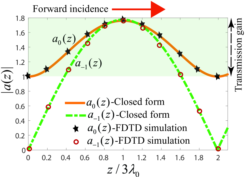
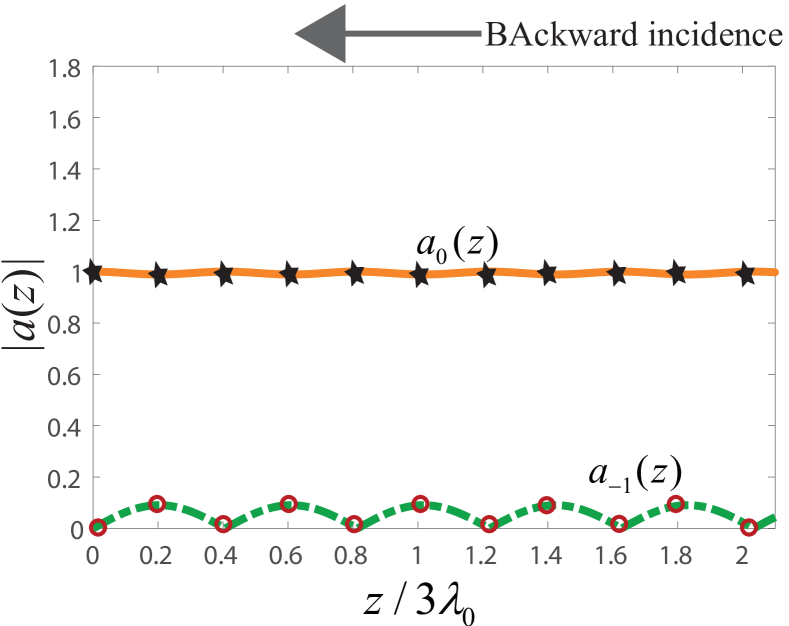
Figure 8: Closed-form solution results and the FDTD numerical simulation results for the $z$-dependent absolute field coefficients in Eq. (13), i.e., $a_{0}(z)$ and $a_{-1}(z)$, inside the superluminal STM beam splitter, with $\gamma=1.2$ and $\delta_{\epsilon}=0.28$. (a) Forward wave incidence, where the wave propagates from left to right. (b) Backward wave incidence, where the wave propagates from right to left.

V.2 Luminal ST Modulation

It may be shown that the for the luminal ST modulation, where $\gamma\rightarrow 1$, the field coefficients in Eq. (15), $a_{0}(z)$ and $a_{-1}(z)$, acquire pure real (or complex) forms. This yields exponential growth of the electric field amplitude along the STM slab. Hence, considering $\gamma=1$, the total electric field inside the STM slab reads

$$E_{\text{S}}(x,z,t) |_{\gamma=1}=E_{0}\cosh\left(\frac{\delta k_{0}^{2}}{4k_{z}}z\right)e^{-i\left(k_{x}x+k_{z}z-\omega_{0}t\right)}$$ (18)

$$-i\frac{\delta k_{0}^{2}}{2k_{z}}E_{0}\sinh\left(\frac{\delta k_{0}^{2}}{4k_{z}}z\right)e^{i\left(-k_{x}x+(q-k_{z})z-\omega_{0}t\right)}.$$

Figure 9 plots the closed form and FDTD numerical simulation results for the absolute value of the electric field coefficients $a_{0}(z)$ and $a_{-1}(z)$ inside the luminal ($\gamma=1$ and $\delta_{\epsilon}=0.28$) STM slab for forward wave incidence. It may be seen from this figure that both $a_{0}(z)$ and $a_{-1}(z)$ possess a non-periodic exponentially growing profile and exhibit a substantial transmission gain at $z\geq 3\lambda_{0}$. It should be noted that, the solution for the field coefficients presented in Eqs. (15) and (S21) are very useful and provide a deep insight into the wave propagation inside the STM slab, especially for the luminal ST modulation (sonic regime), where the Bloch-Floquet-based analytical solution does not exist since the solution does not converge Cassedy and Oliner (1963); Taravati et al. (2017); Taravati (2018a).

Figure 9 plots the result for the luminal STM slab in Fig. 9, except for wave incidence from the right side (backward incidence). It may be seen from this figure that, in contrast to the forward wave incidence, here the incident wave passes through the slab with negligible alteration and minor transition of energy and momentum to the $m=-1$ ST harmonic.

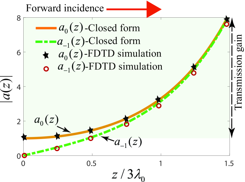
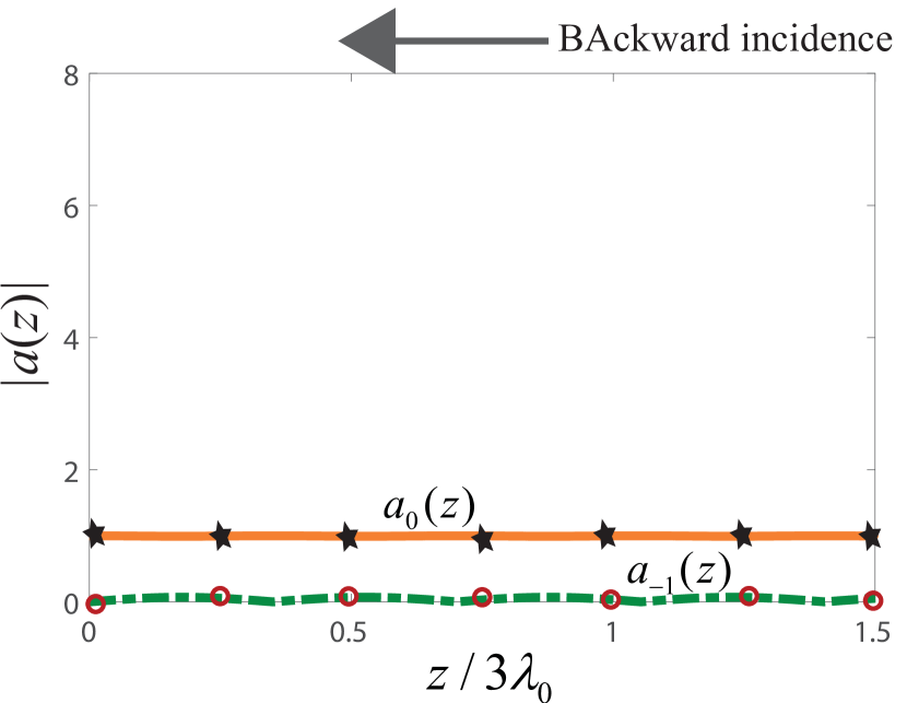
Figure 9: Closed-form solution results and the FDTD numerical simulation results for the $z$-dependent absolute field coefficients in Eq. (13), i.e., $a_{0}(z)$ and $a_{-1}(z)$, inside the luminal STM beam splitter, with $\gamma=1$ and $\delta_{\epsilon}=0.28$. (a) Forward wave incidence, where the wave propagates from left to right. (b) Backward wave incidence, where the wave propagates from right to left.

VI Discussion on Practical realization of Superluminal ST Modulation

To practically realize superluminal ST modulation (here $\gamma=1.2$), the phase velocity of the modulation should be greater than the velocity of the incident wave in the background (unmodulated) medium and not the velocity of light in vacuum Cassedy (1967). Considering a glass as the background medium with permittivity$>1.5$, achieving $\gamma=1.2$ would be realistic. For instance, one may use coupled structures with two different lines (possessing different phase velocities) for the input wave and the modulation Okwit and Sard (1961); Taravati and Caloz (2017); Taravati (2017). In such structures a modulation velocity greater than at least one of the characteristic velocities involved is required. In general, the way of achieving the fast pumping depends on the frequency range, as follows.

• At low frequencies, one may use filter constants which are appropriately selected for two weakly coupled transmission lines Okwit and Sard (1961); Taravati and Caloz (2017); Taravati et al. (2017); Taravati (2017), one for the pump and one for the main incident wave.

• At ultra-high frequencies, a serpentine transmission line msupports the propagation of the main incident wave Okwit et al. (1962), which lowers the phase velocity relative to the modulation velocity.

• At microwave frequencies the pump wave is supported in a closed waveguide Hsu (1960), thereby achieving a fast phase velocity.

In addition, recently, there has been an experimental demonstration of time-modulated structure Reyes-Ayona and Halevi (2016), where the medium is periodically modulated in time only, representing the limiting case of an infinite modulation velocity, i.e., $q=0$ and hence $v_{\text{m}}=\Omega/q\rightarrow\infty$.

VII Conclusion

We have introduced a unidirectional beam splitter and amplifier based on asymmetric coherent photonic transitions in obliquely illuminated space-time-modulated (STM) media. The operation of this dynamic beam splitter is demonstrated by both the analytical, closed-form and numerical simulation results. While the normally illuminated STM media have been previously used for the realization of various components, including insulators, parametric amplifiers and nonreciprocal frequency generators, this paper presented the first study investigating the oblique illumination of STM media. Accordingly, this paper proposed a forward-looking application of such dynamic media. The proposed unidirectional beam splitter is endowed with unique functionalities, including adjustable one-way transmission gain, tunable splitting angle and arbitrary unequal splitting power ratio, as well as high isolation, and hence, is expected to substantially reduce the source and isolation requirements of communication systems.

SUPPLEMENTAL MATERIAL

The beam splitter is placed between $z=0$ and $z=d$, and represented by the space-time-varying permittivity of

$$\epsilon(z,t)=\epsilon_{\text{av}}+\delta_{\epsilon}\sin(qz-\Omega t),$$ (S1)

where $\Omega=2\omega_{\text{0}}$ and

$$q=\frac{2k_{z}}{\gamma}.$$ (S2)

The electric field inside the beam splitter is defined based on the superposition of the $m=0$ and $m=-1$ space-time harmonics fields, i.e.,

$$E_{\text{S}}(x,z,t)=a_{0}(z)e^{-i\left(k_{x}x+k_{z}z-\omega_{0}t\right)}+a_{-1}(z)e^{i\left(-k_{x}x+(q-k_{z})z-\omega_{0}t\right)},$$ (S3)

and the corresponding wave equation reads

$$\frac{\partial^{2}\textbf{E}}{\partial x^{2}}+\frac{\partial^{2}\textbf{E}}{\partial z^{2}}=\frac{1}{c^{2}}\frac{\partial^{2}[\epsilon_{\text{eq}}(t,z)\textbf{E}]}{\partial t^{2}}.$$ (S4)

Inserting the electric field in (S3) into the wave equation in (S4) results in

$$\begin{split}&\left(\frac{\partial^{2}}{\partial x^{2}}+\frac{\partial^{2}}{\partial z^{2}}\right)\left[a_{0}(z)e^{-i\left(k_{x}x+k_{z}z-\omega_{0}t\right)}+a_{-1}(z)e^{i\left(-k_{x}x+(q-k_{z})z-\omega_{0}t\right)}\right]\\ &=\frac{1}{c^{2}}\frac{\partial^{2}}{\partial t^{2}}\left(\bigg{[}\epsilon_{\text{av}}+\frac{\delta}{2}e^{i(qz-2\omega_{\text{0}}t)}+\frac{\delta}{2}e^{-i(qz-2\omega_{\text{0}}t)}\right]\left(a_{0}(z)e^{-i\left(k_{x}x+k_{z}z-\omega_{0}t\right)}+a_{-1}(z)e^{i\left(-k_{x}x+(q-k_{z})z-\omega_{0}t\right)}\right)\bigg{)},\end{split}$$ (S5)

and applying the space and time derivatives, while using a slowly varying envelope approximation, yields

$$\begin{split}&\left[(k_{x}^{2}+k_{z}^{2})a_{0}(z)-2ik_{z}\frac{\partial a_{0}(z)}{\partial z}\right]e^{-i\left(k_{x}x+k_{z}z-\omega_{0}t\right)}\\ &\qquad+\left[(k_{x}^{2}+(q-k_{z})^{2})a_{-1}(z)-2i(k_{z}-q)\frac{\partial a_{-1}(z)}{\partial z}\right]e^{i\left(-k_{x}x+(q-k_{z})z-\omega_{0}t\right)}\\ &\qquad\qquad\qquad\qquad=\frac{\omega_{0}^{2}}{c^{2}}\left(\bigg{[}\epsilon_{\text{av}}+\frac{\delta}{2}e^{i(qz-2\omega_{0}t)}+9\frac{\delta}{2}e^{-i(qz-2\omega_{0}t)}\right]a_{0}(z)e^{-i\left(k_{x}x+k_{z}z-\omega_{0}t\right)}\\ &\qquad\qquad\qquad\qquad\qquad+\left[\epsilon_{\text{av}}+9\frac{\delta}{2}e^{i(qz-2\omega_{0}t)}+\frac{\delta}{2}e^{-i(qz-2\omega_{0}t)}\right]a_{-1}(z)e^{i\left(-k_{x}x+(q-k_{z})z-\omega_{0}t\right)}\bigg{)},\end{split}$$ (S6)

We then multiply both sides of Eq. (S6) with $e^{i\left(k_{x}x+k_{z}z-\omega_{0}t\right)}$, which gives

$$\begin{split}&\left[(k_{x}^{2}+k_{z}^{2})a_{0}(z)-2ik_{z}\frac{\partial a_{0}(z)}{\partial z}\right]+\left[(k_{x}^{2}+(q-k_{z})^{2})a_{-1}(z)-2i(k_{z}-q)\frac{\partial a_{-1}(z)}{\partial z}\right]e^{i\left(qz-2\omega_{0}t\right)}\\ &=\frac{\omega_{0}^{2}}{c^{2}}\left(\bigg{[}\epsilon_{\text{av}}+\frac{\delta}{2}e^{i(qz-2\omega_{0}t)}+9\frac{\delta}{2}e^{-i(qz-2\omega_{0}t)}\right]a_{0}(z)+\left[\epsilon_{\text{av}}e^{i(qz-2\omega_{0}t)}+9\frac{\delta}{2}e^{i2(qz-2\omega_{0}t)}+\frac{\delta}{2}\right]a_{-1}(z)\bigg{)},\end{split}$$ (S7)

and next, applying $\int_{0}^{\frac{\pi}{\omega_{0}}}dt$ to both sides of (S7) yields

$$\frac{da_{0}(z)}{dz}=\frac{ik_{0}^{2}}{2k_{z}}\left(\left[\epsilon_{\text{av}}-\epsilon_{\text{r}}\right]a_{0}(z)+\frac{\delta}{2}a_{-1}(z)\right),$$ (S8)

which may be cast as

$$\frac{da_{0}(z)}{dz}=M_{0}a_{0}(z)+C_{0}a_{-1}(z),$$ (S9)

where

$$M_{0}=\frac{ik_{0}^{2}}{2k_{z}}(\epsilon_{\text{av}}-\epsilon_{\text{r}}),\qquad C_{0}=\frac{i\delta k_{0}^{2}}{4k_{z}}.$$ (S10)

Following the same procedure, we next multiply both sides of (S7) with $e^{-i\left(qz-2\omega_{0}t\right)}$, and applying $\int_{0}^{\frac{\pi}{\omega_{0}}}dt$ in both sides of the resultant, which reduces to

$$\left[(k_{x}^{2}+(q-k_{z})^{2})a_{-1}(z)-2i(k_{z}-q)\frac{\partial a_{-1}(z)}{\partial z}\right]=\frac{\omega_{0}^{2}}{c^{2}}\left(\frac{\delta}{2}a_{0}(z)+\epsilon_{\text{av}}a_{-1}(z)\right),$$ (S11)

which may be cast as

$$\frac{da_{-1}(z)}{dz}=C_{-1}a_{0}(z)+M_{-1}a_{-1}(z),$$ (S12)

where

$$M_{-1}=\frac{ik_{0}^{2}}{2(k_{z}-q)}\left[\epsilon_{\text{av}}-\epsilon_{\text{r}}\frac{k_{x}^{2}+(q-k_{z})^{2}}{k_{0}^{2}}\right],\qquad C_{-1}=\frac{i\delta k_{0}^{2}}{4(k_{z}-q)}$$ (S13)

Equations (S9) and (S12) form a matrix differential equation. We then look for independent differential equations for $a_{0}(z)$ and $a_{-1}(z)$, which is expressed by

$$\frac{d^{2}a_{0}(z)}{dz^{2}}-(M_{0}+M_{-1})\frac{da_{0}(z)}{dz}+(M_{0}M_{-1}-C_{0}C_{-1})a_{0}(z)=0,$$ (S14)

$$\frac{d^{2}a_{-1}(z)}{dz^{2}}-(M_{0}+M_{-1})\frac{da_{-1}(z)}{dz}+(M_{0}M_{-1}-C_{0}C_{-1})a_{-1}(z)=0.$$ (S15)

which are second order differential equations. Using the initial conditions of $a_{0}(0)=E_{0}$ and $a_{-1}(0)=0$ gives

$$a_{0}(z)=\frac{E_{0}}{2\varDelta}\left((M_{0}-M_{-1}+\varDelta)e^{\frac{M_{0}+M_{-1}+\varDelta}{2}z}-(M_{0}-M_{-1}-\varDelta)e^{\frac{M_{0}+M_{-1}-\varDelta}{2}z}\right),$$ (S16)

$$a_{-1}(z)=C_{-1}\frac{E_{0}}{\varDelta}\left(e^{\frac{M_{0}+M_{-1}+\varDelta}{2}z}-e^{\frac{M_{0}+M_{-1}-\varDelta}{2}z}\right),$$ (S17)

where

$$\varDelta=\sqrt{(M_{0}+M_{-1})^{2}-4(M_{0}M_{-1}-C_{0}C_{-1})}=\sqrt{(M_{0}-M_{-1})^{2}+4C_{0}C_{-1}}.$$ (S18)

Assuming an imaginary result for $\varDelta$ (which occurs for subluminal and superluminal space-time modulations), $a_{0}(z)$ and $a_{-1}(z)$ acquire a periodic sinusoidal form, where the maximum amplitude of them occur at the coherence length $z=l_{\text{c}}$, where

$$\frac{d}{dz}a_{0}(z)|_{z=l_{\text{c}}}=\frac{d}{dz}a_{-1}(z)|_{z=l_{\text{c}}}=0,$$ (S19)

which corresponds to

$$l_{\text{c}}=\pi\left(\left[\frac{k_{0}^{2}[\epsilon_{\text{av}}-\epsilon_{\text{r}}]/k_{z}-q}{(k_{z}-q)/(k_{z}-q/2)}\right]^{2}+\frac{\delta^{2}k_{0}^{4}}{4k_{z}(k_{z}-q)}\right)^{-1}.$$ (S20)

For luminal space-time modulation, where $\gamma\rightarrow 1$ and $q\rightarrow 2k_{z}$, $a_{0}(z)$ and $a_{-1}(z)$ acquire exponentially growing profile, and hence, the total electric field inside the slab reads

$$E(x,z,t)=E_{0}\cosh\left(\frac{\delta k_{0}^{2}}{4k_{z}}z\right)e^{-i\left(k_{x}x+k_{z}z-\omega_{0}t\right)}-i\frac{\delta k_{0}^{2}}{2k_{z}}E_{0}\sinh\left(\frac{\delta k_{0}^{2}}{4k_{z}}z\right)e^{i\left(-k_{x}x+(q-k_{z})z-\omega_{0}t\right)},$$ (S21)

which demonstrates the wave amplification of both $m=0$ and $m=-1$ ST harmonics, for the luminal space-time modulation.

References

- Schneider (2014) Christian Schneider, On-chip superconducting microwave beam splitter, Ph.D. thesis, Master’s thesis, Technische Universität München (2014).
- Hammer et al. (2015) Jakob Hammer, Sebastian Thomas, Philipp Weber, and Peter Hommelhoff, “Microwave chip-based beam splitter for low-energy guided electrons,” Phys. Rev. Lett. 114, 254801 (2015).
- Tan and Yassin (2017) Boon-Kok Tan and Ghassan Yassin, “A planar beam splitter for millimeter and submillimeter heterodyne mixer array,” IEEE Transactions on Terahertz Science and Technology 7, 664–668 (2017).
- Watanabe (1980) Ryuichi Watanabe, “A novel polarization-independent beam splitter,” IEEE Trans. Microw. Theory Techn. 28, 685–689 (1980).
- Zhu et al. (2006) W Zhu, J Shaker, JS Wight, M Cuhaci, and DA McNamara, “Microwave spatial beam splitter/combiner using artificial microwave volume hologram technology,” Electronics Letters 42, 1 (2006).
- Hwang et al. (2012) Ruey-Bing Hwang, Neng-Chieh Hsu, and Cheng-Yuan Chin, “A spatial beam splitter consisting of a near-zero refractive index medium,” IEEE Trans. Antennas Propagat. 60, 417–420 (2012).
- Cooper et al. (2012) James R Cooper, Sangkil Kim, and Manos M Tentzeris, “A novel polarization-independent, free-space, microwave beam splitter utilizing an inkjet-printed, 2-D array frequency selective surface,” IEEE Antennas Wirel. Propagat. Lett. 11, 686–688 (2012).
- Wallraff et al. (2004) Andreas Wallraff, David I Schuster, Alexandre Blais, L Frunzio, R-S Huang, J Majer, S Kumar, Steven M Girvin, and Robert J Schoelkopf, “Strong coupling of a single photon to a superconducting qubit using circuit quantum electrodynamics,” Nature 431, 162 (2004).
- Blais et al. (2004) Alexandre Blais, Ren-Shou Huang, Andreas Wallraff, Steven M Girvin, and R Jun Schoelkopf, “Cavity quantum electrodynamics for superconducting electrical circuits: An architecture for quantum computation,” Phys. Rev. A 69, 062320 (2004).
- Mariantoni et al. (2008) Matteo Mariantoni, Frank Deppe, Achim Marx, Rudolf Gross, Frank K Wilhelm, and Enrique Solano, “Two-resonator circuit quantum electrodynamics: A superconducting quantum switch,” Phys. Rev. B 78, 104508 (2008).
- Houck et al. (2007) AA Houck, DI Schuster, JM Gambetta, JA Schreier, BR Johnson, JM Chow, L Frunzio, J Majer, MH Devoret, SM Girvin, et al., “Generating single microwave photons in a circuit,” Nature 449, 328 (2007).
- Bozyigit et al. (2011a) D Bozyigit, C Lang, L Steffen, JM Fink, C Eichler, M Baur, R Bianchetti, PJ Leek, S Filipp, A Wallraff, et al., “Correlation measurements of individual microwave photons emitted from a symmetric cavity,” in Journal of Physics: Conference Series, Vol. 264 (IOP Publishing, 2011) p. 012024.
- Bozyigit et al. (2011b) D Bozyigit, C Lang, L Steffen, JM Fink, C Eichler, M Baur, R Bianchetti, PJ Leek, S Filipp, MP Da Silva, et al., “Antibunching of microwave-frequency photons observed in correlation measurements using linear detectors,” Nature Physics 7, 154 (2011b).
- Mariantoni et al. (2010) Matteo Mariantoni, Edwin P Menzel, Frank Deppe, MA Araque Caballero, Alexander Baust, Thomas Niemczyk, Elisabeth Hoffmann, Enrique Solano, Achim Marx, and Rudolf Gross, “Planck spectroscopy and quantum noise of microwave beam splitters,” Phys. Rev. Lett. 105, 133601 (2010).
- Cassedy (1967) E. S. Cassedy, “Dispersion relations in time-space periodic media: part II-unstable interactions,” Proc. IEEE 55, 1154 – 1168 (1967).
- Yu and Fan (2009) Z. Yu and S. Fan, “Complete optical isolation created by indirect interband photonic transitions,” Nat. Photonics 3, 91 – 94 (2009).
- Taravati (2018a) Sajjad Taravati, “Giant linear nonreciprocity, zero reflection, and zero band gap in equilibrated space-time-varying media,” Phys. Rev. Appl. 9, 064012 (2018a).
- Taravati et al. (2017) Sajjad Taravati, Nima Chamanara, and Christophe Caloz, “Nonreciprocal electromagnetic scattering from a periodically space-time modulated slab and application to a quasisonic isolator,” Phys. Rev. B 96, 165144 (2017).
- Salary et al. (2018a) Mohammad Mahdi Salary, Samad Jafar-Zanjani, and Hossein Mosallaei, “Time-varying metamaterials based on graphene-wrapped microwires: Modeling and potential applications,” Phys. Rev. B 97, 115421 (2018a).
- Salary et al. (2018b) Mohammad Mahdi Salary, Samad Jafar-Zanjani, and Hossein Mosallaei, “Electrically tunable harmonics in time-modulated metasurfaces for wavefront engineering,” New Journal of Physics (2018b).
- Taravati and Kishk (2019) Sajjad Taravati and Ahmed A. Kishk, “Advanced wave engineering via obliquely illuminated space-time-modulated slab,” IEEE Trans. Antennas Propagat. 67, 270–281 (2019).
- Cullen (1958) A. L. Cullen, “A travelling-wave parametric amplifier,” Nature 181, 332 (1958).
- Tien (1958) P. K. Tien, “Parametric amplification and frequency mixing in propagating circuits,” J. Appl. Phys. 29, 1347–1357 (1958).
- Tien and Suhl (1958) PK Tien and H Suhl, “A traveling-wave ferromagnetic amplifier,” Proceedings of the IRE 46, 700–706 (1958).
- Cassedy and Oliner (1963) E. S. Cassedy and A. A. Oliner, “Dispersion relations in time-space periodic media: part I-stable interactions,” Proc. IEEE 51, 1342 – 1359 (1963).
- Wentz (1966) JL Wentz, “A nonreciprocal electrooptic device,” Proceedings of the IEEE 54, 97–98 (1966).
- Bhandare et al. (2005) Suhas Bhandare, Selwan K Ibrahim, David Sandel, Hongbin Zhang, F Wust, and Reinhold Noé, “Novel nonmagnetic 30-dB traveling-wave single-sideband optical isolator integrated in III/V material,” IEEE J. Sel. Top. Quantum Electron. 11, 417–421 (2005).
- Lira et al. (2012) H. Lira, Z. Yu, S. Fan, and M. Lipson, “Electrically driven nonreciprocity induced by interband photonic transition on a silicon chip,” Phys. Rev. Lett. 109, 033901 (2012).
- Chamanara et al. (2017) Nima Chamanara, Sajjad Taravati, Zoé-Lise Deck-Léger, and Christophe Caloz, “Optical isolation based on space-time engineered asymmetric photonic bandgaps,” Phys. Rev. B 96, 155409 (2017).
- Taravati (2017) Sajjad Taravati, “Self-biased broadband magnet-free linear isolator based on one-way space-time coherency,” Phys. Rev. B 96, 235150 (2017).
- Kim et al. (2017) JunHwan Kim, Seunghwi Kim, and Gaurav Bahl, “Complete linear optical isolation at the microscale with ultralow loss,” Scientific reports 7, 1647 (2017).
- Sohn et al. (2018) Donggyu B Sohn, Seunghwi Kim, and Gaurav Bahl, “Time-reversal symmetry breaking with acoustic pumping of nanophotonic circuits,” Nat. Photon. 12, 91 (2018).
- Hadad et al. (2015) Y. Hadad, D. L. Sounas, and A. Alù, “Space-time gradient metasurfaces,” Phys. Rev. B 92, 100304 (2015).
- Shi and Fan (2016) Y. Shi and S. Fan, “Dynamic non-reciprocal meta-surfaces with arbitrary phase reconfigurability based on photonic transition in meta-atoms,” Appl. Phys. Lett. 108, 021110 (2016).
- Shi et al. (2017) Yu Shi, Seunghoon Han, and Shanhui Fan, “Optical circulation and isolation based on indirect photonic transitions of guided resonance modes,” ACS Photonics 4, 1639–1645 (2017).
- Wu and Grbic (2018) Zhanni Wu and Anthony Grbic, “A transparent, time-modulated metasurface,” in 2018 12th International Congress on Artificial Materials for Novel Wave Phenomena (Metamaterials) (IEEE, 2018) pp. 439–441.
- Taravati (2018b) Sajjad Taravati, “Aperiodic space-time modulation for pure frequency mixing,” Phys. Rev. B 97, 115131 (2018b).
- Qin et al. (2014) Shihan Qin, Qiang Xu, and Yuanxun Ethan Wang, “Nonreciprocal components with distributedly modulated capacitors,” IEEE Trans. Microw. Theory Techn. 62, 2260–2272 (2014).
- Estep et al. (2014) Nicholas A Estep, Dimitrios L Sounas, Jason Soric, and Andrea Alù, “Magnetic-free non-reciprocity and isolation based on parametrically modulated coupled-resonator loops,” Nat. Phys. 10, 923–927 (2014).
- Reiskarimian et al. (2018) Negar Reiskarimian, Aravind Nagulu, Tolga Dinc, and Harish Krishnaswamy, “Integrated conductivity-modulation-based rf magnetic-free non-reciprocal components: Recent results and benchmarking,” arXiv preprint arXiv:1805.11662 (2018).
- Taravati and Caloz (2015) S. Taravati and C. Caloz, “Space-time modulated nonreciprocal mixing, amplifying and scanning leaky-wave antenna system,” in IEEE AP-S Int. Antennas Propagat. (APS) (Vancouver, Canada, 2015).
- Taravati and Caloz (2017) Sajjad Taravati and Christophe Caloz, “Mixer-duplexer-antenna leaky-wave system based on periodic space-time modulation,” IEEE Trans. Antennas Propagat. 65, 442 – 452 (2017).
- (43) See Supplemental Material for detailed derivations.
- Okwit and Sard (1961) S Okwit and EW Sard, “Constant-output-frequency, octave tuning range backward-wave parametric amplifier,” IRE Transactions on Electron Devices 8, 540–549 (1961).
- Okwit et al. (1962) S Okwit, MI Grace, and EW Sard, “UHF backward-wave parametric amplifier,” IRE Transactions on Microwave Theory and Techniques 10, 558–563 (1962).
- Hsu (1960) Hsiung Hsu, “Backward traveling-wave parametric amplifiers,” in Solid-State Circuits Conference. Digest of Technical Papers. 1960 IEEE International, Vol. 3 (IEEE, 1960) pp. 91–92.
- Reyes-Ayona and Halevi (2016) José Roberto Reyes-Ayona and Peter Halevi, “Electromagnetic wave propagation in an externally modulated low-pass transmission line,” IEEE Transactions on Microwave Theory and Techniques 64, 3449–3459 (2016).