GAUSS-BONNET GRAVITY IN $D=4$ WITHOUT GAUSS-BONNET COUPLING TO MATTER – COSMOLOGICAL IMPLICATIONS

Abstract

We propose a new model of $D=4$ Gauss-Bonnet gravity. To avoid the usual property of the integral over the standard $D=4$ Gauss-Bonnet scalar becoming a total derivative term, we employ the formalism of metric-independent non-Riemannian spacetime volume elements which makes the $D=4$ Gauss-Bonnet action term non-trivial without the need to couple it to matter fields unlike the case of ordinary $D=4$ Gauss-Bonnet gravity models. The non-Riemannian volume element dynamically triggers the Gauss-Bonnet scalar to be an arbitrary integration constant $M$ on-shell, which in turn has several interesting cosmological implications: (i) It yields specific solutions for the Hubble parameter and the Friedmann scale factor as functions of time, which are completely independent of the matter dynamics, i.e., there is no back reaction by matter on the cosmological metric. (ii) For $M>0$ it predicts a “coasting”-like evolution immediately after the Big Bang, and it yields a late universe with dynamically produced dark energy density given through $M$; (iii) For the special value $M=0$ we obtain exactly a linear “coasting” cosmology; (iv) For $M<0$ we have in addition to the Big Bang also a Big Crunch with “coasting”-like evolution around both; (v) It allows for an explicit analytic solution of the pertinent Friedmann and $\phi$ scalar field equations of motion, while dynamically fixing uniquely the functional dependence on $\phi$ of the scalar potential.

Received (Day Month Year)Revised (Day Month Year)

PACS Nos.: 04.50.Kd, 98.80.Jk, 95.36.+x.

1 Introduction

Extended gravity theories as alternatives/generalizations of the standard Einstein General Relativity (for detailed accounts, see Ref. extended-grav,extended-grav-book,odintsov-1,odintsov-2 and references therein) enjoy a very active development in the last decade or so due to pressing motivation from various areas: cosmology (problems of dark energy and dark matter), quantum field theory in curved spacetime (renormalization in higher loops), string theory (low-energy effective field theories).

When considering alternative/extended theories to General Relativity, one option is to employ alternative non-Riemannian spacetime volume-forms (metric-independent generally covariant volume elements or integration measure densities) in the pertinent Lagrangian actions instead of the canonical Riemannian one given by the square-root of the determinant of the Riemannian metric.

To this end let us briefly recall the essential features of the formalism of non-Riemannian spacetime volume-forms, which are defined in terms of auxiliary antisymmetric tensor gauge fields of maximal rank. This formalism is the basis for constructing a series of extended gravity-matter models describing unified dark energy and dark matter scenario [5], quintessential cosmological models with gravity-assisted and inflaton-assisted dynamical generation or suppression of electroweak spontaneous symmetry breaking and charge confinement [6, 7, 8], and a novel mechanism for the supersymmetric Brout-Englert-Higgs effect in supergravity [9] (see Ref. susyssb-1,grav-bags for a consistent geometrical formulation of the non-Riemannian volume-form approach, which is an extension of the originally proposed method [11, 12]).

Volume-forms (generally-covariant integration measures) in integrals over manifolds are given by nonsingular maximal rank differential forms $\omega$:

$$\int_{{\mathcal{M}}}\omega\bigl{(}\ldots\bigr{)}=\int_{{\mathcal{M}}}dx^{D}\,\Omega\bigl{(}\ldots\bigr{)}\;\;,\;\;\omega=\frac{1}{D!}\omega_{\mu_{1}\ldots\mu_{D}}dx^{\mu_{1}}\wedge\ldots\wedge dx^{\mu_{D}}\;,$$ (1)

$$\omega_{\mu_{1}\ldots\mu_{D}}=-\varepsilon_{\mu_{1}\ldots\mu_{D}}\Omega\;\;,\;\;dx^{\mu_{1}}\wedge\ldots\wedge dx^{\mu_{D}}=\varepsilon^{\mu_{1}\ldots\mu_{D}}\,dx^{D}\;,$$ (2)

(our conventions for the alternating symbols $\varepsilon^{\mu_{1},\ldots,\mu_{D}}$ and $\varepsilon_{\mu_{1},\ldots,\mu_{D}}$ are: $\varepsilon^{01\ldots D-1}=1$ and $\varepsilon_{01\ldots D-1}=-1$). The volume element (integration measure density) $\Omega$ transforms as scalar density under general coordinate reparametrizations.

In standard generally-covariant theories (with action $S=\int d^{D}\!x\sqrt{-g}{\mathcal{L}}$) the Riemannian spacetime volume-form is defined through the “D-bein” (frame-bundle) canonical one-forms $e^{A}=e^{A}_{\mu}dx^{\mu}$ ($A=0,\ldots,D-1$), related to the Riemannian metric ($g_{\mu\nu}=e^{A}_{\mu}e^{B}_{\nu}\eta_{AB}$ , $\eta_{AB}\equiv{\rm diag}(-1,1,\ldots,1)$):

$$\omega=e^{0}\wedge\ldots\wedge e^{D-1}=\det\|e^{A}_{\mu}\|\,dx^{\mu_{1}}\wedge\ldots\wedge dx^{\mu_{D}}$$

$$\longrightarrow\quad\Omega=\det\|e^{A}_{\mu}\|\,d^{D}x=\sqrt{-\det\|g_{\mu\nu}\|}\,d^{D}x\;.$$ (3)

We will employ (Section 2 below) instead of $\sqrt{-g}$ another alternative non-Riemannian volume element as in (1)-(2) given by a non-singular exact $D$-form $\omega=d{\mathcal{C}}$ where:

$${\mathcal{C}}=\frac{1}{(D-1)!}C_{\mu_{1}\ldots\mu_{D-1}}dx^{\mu_{1}}\wedge\ldots\wedge dx^{\mu_{D-1}}\;,$$ (4)

so that the non-Riemannian volume element reads:

$$\Omega\equiv\Phi(C)=\frac{1}{(D-1)!}\varepsilon^{\mu_{1}\ldots\mu_{D}}\,\partial_{\mu_{1}}C_{\mu_{2}\ldots\mu_{D}}\;.$$ (5)

Here $C_{\mu_{1}\ldots\mu_{D-1}}$ is an auxiliary rank $(D-1)$ antisymmetric tensor gauge field. $\Phi(C)$, which is in fact the density of the dual of the rank $D$ field-strength $F_{\mu_{1}\ldots\mu_{D}}=\frac{1}{(D-1)!}\partial_{[\mu_{1}}C_{\mu_{2}\ldots\mu_{D}]}=-\varepsilon_{\mu_{1}\ldots\mu_{D}}\Phi(C)$, similarly transforms as scalar density under general coordinate reparametrizations. Let us note that the non-Riemannian volume element $\Phi(C)$ is dimensionless like the standard Riemannian one $\sqrt{-g}$, meaning that the auxialiary antisymmetric tensor gauge field $C_{\mu_{1}\ldots\mu_{D-1}}$ has dimension 1 in units of length.

Now, it is clear that if we replace the usual Riemannian volume element $\sqrt{-g}$ with a non-Riemannian one $\Phi(C)$ in the Lagrangian action integral over the Gauss-Bonnet scalar $\int d^{4}x\,\Phi(C)\,R^{2}_{\rm GB}$ (Eqs.(6)-(7) below), then the latter will cease to be a total derivative in $D=4$. Thus, we will avoid the necessity to couple $R^{2}_{\rm GB}$ in $D=4$ directly to matter fields or to use nonlinear functions of $R^{2}_{\rm GB}$ unlike the usual $D=4$ Gauss-Bonnet gravity – for reviews, see Ref. GB-grav-3,GB-grav-4; for recent discussions of Gauss-Bonnet cosmology, see Ref. GB-grav-cosmolog-1-GB-grav-cosmolog-10) and references therein.

The main new feature, displayed in Section 2, of our non-standard $D=4$ Gauss-Bonnet gravity with a Gauss-Bonnet action term $\int d^{4}x\,\Phi(C)R^{2}_{\rm GB}$ is due to the equation of motion w.r.t. auxiliary tensor gauge field defining $\Phi(C)$ as in (5), namely it dynamically triggers the Gauss-Bonnet scalar $R^{2}_{\rm GB}$ to be on-shell an arbitrary integration constant (Eq.(15) below). The latter property has, however, a consequence – now the composite field $\chi=\frac{\Phi(C)}{\sqrt{-g}}$ appears as an additional physical field degree of freedom related to the geometry of spacetime and its role in the cosmological setting is described below. Let us note that this is in sharp contrast w.r.t. other extended gravity-matter models constructed in terms of (one or several) non-Riemannian volume forms [9, 10, 5, 6, 7, 8], where we start within the first-order formalism and where composite fields of the type of $\chi$ turn out to be (almost) pure gauge (non-propagating) degrees of freedom.

The dynamically triggered constancy of $R^{2}_{\rm GB}$ in turn has several interesting implications for cosmology.

As we will show in Section 3 below, the cosmological dynamics in the new $D=4$ Gauss-Bonnet gravity provides automatically a “coasting” evolution of the early universe near the Big Bang at $t=t_{\rm BB}$, where the Hubble parameter $H(t)\sim(t-t_{\rm BB})^{-1}$ and the Friedmann scale factor $a(t)\sim(t-t_{\rm BB})$, i.e., space size $a(t)$ and horizon size $H^{-1}(t)$ expand at the same rate (no horizon problem); for a general discussion of “coasting” cosmological evolution, see Ref. coasting-1-coasting-4. Furthermore, for late times we obtain either a de Sitter universe with dynamically generated dark energy density or a Big Crunch depending on the sign of the dynamically generated constant value of $R^{2}_{\rm GB}$.

An important observation here is that the cosmological solution for $H(t)$ and $a(t)$ does not feel the details of the matter content and the matter dynamics, i.e., there is no direct back reaction of matter on the cosmological metric. The reason here is that the differential equation determining the solution $H(t)$ (or $a(t)$) results from the equation for the Gauss-Bonnet scalar equalling arbitrary integration constant on-shell, which does not involve any matter terms. On the other hand, matter terms are present in the pertinent Friedmann equations (Section 3) which now reduce to a differential equation for the composite field $\chi=\Phi(C)/\sqrt{-g}$. Therefore, the solution for $\chi$ (Eq.(26) below) completely absorbs the impact of the matter dynamics while the overall solution for $H(t)$ and $a(t)$ is left unchanged. Furthermore, if we “freeze” $\chi$ to be a constant (Section 4 below), then in the case of scalar field $\phi$ matter the exact expression for the corresponding scalar potential $V(\phi)$ as function of $\phi$ is fixed uniquely.

The above described main properties of the present version of $D=4$ Gauss-Bonnet gravity, namely, the dynamical constancy of the Gauss-Bonnet scalar derived from a Lagrangian action principle and the appearance of an additional degree of freedom $\chi$ absorbing the effect of the matter dynamics, are the most significant differences w.r.t. the approach in several recent papers [29, 30, 31] extensively studying static spherically symmetric solutions in gravitational theories in the presence of a constant Gauss-Bonnet scalar, where the constancy of the latter is imposed as an additional condition on-shell beyond the standard equations of motion resulting from an action principle.

In the last discussion section we point out a limitation of the present non-canonical $D=4$ Einstein-Gauss-Bonnet model, namely, that it predicts continuous acceleration throughout the whole evolution of the universe, and we briefly describe a generalization of our model allowing for both acceleration and deceleration.

2 Gauss-Bonnet Gravity in $D=4$ With a Non-Riemannian Volume Element

We propose the following self-consistent action of $D=4$ Gauss-Bonnet gravity without the need to couple the Gauss-Bonnet scalar to some matter fields (for simplicity we are using units with the Newton constant $G_{N}=1/16\pi$):

$$S=\int d^{4}x\sqrt{-g}\Bigl{[}R+L_{\rm matter}\Bigr{]}+\int d^{4}x\,\Phi(C)\,R_{\rm GB}^{2}\;.$$ (6)

Here the notations used are as follows (we employ the usual second order formalism):

• $R_{\rm GB}^{2}$ denotes the Gauss-Bonnet scalar:

  $$R_{\rm GB}^{2}\equiv R^{2}-4R_{\mu\nu}R^{\mu\nu}+R_{\mu\nu\kappa\lambda}R^{\mu\nu\kappa\lambda}\;.$$ (7)

• $\Phi(C)$ denotes a non-Riemannian volume element defined as a scalar density of the dual field-strength of an auxiliary antisymmetric tensor gauge field of maximal rank $C_{\mu\nu\lambda}$:

  $$\Phi(C)=\frac{1}{3!}\varepsilon^{\mu\nu\kappa\lambda}\partial_{\mu}C_{\nu\kappa\lambda}\;.$$ (8)

  Let us particularly stress that, although we stay in $D=4$ spacetime dimensions and although we don’t couple the Gauss-Bonnet scalar (7) to the matter fields, the last term in (6) thanks to the presence of the non-Riemannian volume element (8) is non-trivial (not a total derivative as with the ordinary Riemannian volume element $\sqrt{-g}$)) and yields a non-rivial contribution to the Einstein equations (Eqs.(11) below).

• As a matter Lagrangian we will take for simplicity an ordinary scalar field one:

  $$L_{\rm matter}=-\frac{1}{2}g^{\mu\nu}\partial_{\mu}\phi\partial_{\nu}\phi-V(\phi)\;.$$ (9)

  As discussed below, the explicit choice of $L_{\rm matter}$ does not affect the cosmological solutions for the Hubble parameter and the Friedmann scale factor. It only affects the solution for the composite field $\chi$ defined in Eq.(10) (cf. Eq.(26) below).

We now have three types of equations of motion resulting from the action (6):

• Einstein equations w.r.t. $g^{\mu\nu}$ where we employ the definition for a dimensionelss composite field:

  $$\chi\equiv\frac{\Phi(C)}{\sqrt{-g}}$$ (10)

  representing the ratio of the non-Riemannian to the standard Riemannian volume element:

  $$R_{\mu\nu}-\frac{1}{2}g_{\mu\nu}R=\frac{1}{2}T_{\mu\nu}-\frac{1}{2}g_{\mu\nu}\chi R_{\rm GB}^{2}+2R\nabla_{\mu}\nabla_{\nu}\chi$$

  $$+4\Box\chi\bigl{(}R_{\mu\nu}-\frac{1}{2}g_{\mu\nu}R\bigr{)}-4R_{\mu}^{\rho}\nabla_{\rho}\nabla_{\nu}\chi-4R_{\nu}^{\rho}\nabla_{\rho}\nabla_{\mu}\chi$$

  $$+4g_{\mu\nu}R^{\rho\sigma}\nabla_{\rho}\nabla_{\sigma}\chi-4g^{\kappa\rho}g^{\lambda\sigma}R_{\mu\kappa\nu\lambda}\nabla_{\rho}\nabla_{\sigma}\chi\;,$$ (11)

  where $T_{\mu\nu}=g_{\mu\nu}L_{\rm matter}-2\frac{\partial}{\partial g^{\mu\nu}}L_{\rm matter}$ is the standard matter energy-momentum tensor:

  $$T_{\mu\nu}=\partial_{\mu}\phi\partial_{\nu}\phi-g_{\mu\nu}\Bigl{(}\frac{1}{2}g^{\kappa\lambda}\partial_{\kappa}\phi\partial_{\lambda}\phi+V(\phi)\Bigr{)}\;.$$ (12)

• The equations of motion w.r.t. scalar field $\phi$ have the standard form (they are not affected by the presence of the Gauss-Bonnet term):

  $$\Box\phi+\frac{\partial V}{\partial\phi}=0\;.$$ (13)

• The crucial new feature are the equations of motion w.r.t. auxiliary non-Riemannian volume element tensor gauge field $C_{\mu\nu\lambda}$:

  $$0=\frac{\delta}{\delta C_{\nu\kappa\lambda}}\int d^{4}x\Phi(C)R^{2}_{\rm GB}=-\frac{1}{3!}\varepsilon^{\mu\nu\kappa\lambda}\partial_{\mu}R^{2}_{\rm GB}\;,$$ (14)

  that is:

  $$\partial_{\mu}R_{\rm GB}^{2}=0\quad\longrightarrow\quad R_{\rm GB}^{2}=24M={\rm const}\;,$$ (15)

  where $M$ is an arbitrary dimensionful integration constant and the numerical factor 24 in (15) is chosen for later convenience.

The dynamically triggered constancy of the Gauss-Bonnet scalar (15) comes at a price as we see from the generalized Einstein Eqs.(11) – namely, now the composite field $\chi=\frac{\Phi(C)}{\sqrt{-g}}$ appears as an additional physical field degree of freedom.

In what follows we will see (Section 4) that when considering cosmological solutions we can consistently “freeze” the composite field $\chi={\rm const}$ so that all terms on the r.h.s. of (11) with derivatives of the composite field $\chi$ will vanish. The freezing of $\chi$ together with (15) has two main effects:

(a) It produces on r.h.s. of (11) a dynamically generated cosmological constant $\Lambda_{0}$-term:

$$-g_{\mu\nu}\chi R_{\rm GB}^{2}=-g_{\mu\nu}2\Lambda_{0}\;\;,\;\;\Lambda_{0}\equiv 12\chi M\;.$$ (16)

(b) Within the class of cosmological solutions, as shown in Section 4 below, the “freezing” of $\chi$ produces an explicit analytic solution of the extended Friedmann equations and of the $\phi$ scalar field equations of motion, with simultaneous dynamical fixing uniquely of the functional dependence on $\phi$ of the scalar potential $V(\phi)$. In particular it yields the exact value of the vacuum energy density in the “late” universe – the dark energy density (Eq.(55) below) – in terms of the dynamically generated constant value of the Gauss-Bonnet scalar (15).

3 Cosmological Solutions with a Dynamically Constant Gauss-Bonnet Scalar

Now we perform a Friedmann-Lemaitre-Robertson-Walker (FLRW) reduction of the original action (6) with FLRW metric:

$$ds^{2}=g_{\mu\nu}dx^{\mu}dx^{\nu}=-N^{2}(t)dt^{2}+a^{2}(t)d{\vec{x}}^{2}$$ (17)

where:

$$\Phi(C)=\stackrel{{\scriptstyle.}}{{C}}\quad,\quad R_{\rm GB}^{2}=\frac{8}{Na^{3}}\frac{d}{dt}\Bigl{(}\frac{\stackrel{{\scriptstyle.}}{{a}}^{3}}{N^{3}}\Bigr{)}\;,$$ (18)

the overdot denoting $\frac{d}{dt}$. The corresponding FLRW action reads:

$$S_{\rm FLRW}=\int dt\Bigl{\{}-6\frac{a\stackrel{{\scriptstyle.}}{{a}}^{2}}{N}+Na^{3}\bigl{[}\frac{\stackrel{{\scriptstyle.}}{{\phi}}^{2}}{2N^{2}}-V(\phi)\bigr{]}+\frac{8\stackrel{{\scriptstyle.}}{{C}}}{Na^{3}}\frac{d}{dt}\Bigl{(}\frac{\stackrel{{\scriptstyle.}}{{a}}^{3}}{N^{3}}\Bigr{)}\Bigr{\}}\;.$$ (19)

Accordingly, the equations of motion of (19) – FLRW counterparts of Eqs.(15),(11),(13) – acquire the form (as usual, after variation w.r.t. lapse function $N(t)$ we set the gauge $N(t)=1$):

• The FLRW counterpart of (15) (the constancy of Gauss-Bonnet scalar) becomes:

  $$\frac{\stackrel{{\scriptstyle.}}{{a}}^{2}}{a^{2}}\,\frac{\stackrel{{\scriptstyle..}}{{a}}}{a}=M\quad\longrightarrow\quad\stackrel{{\scriptstyle.}}{{H}}=-H^{2}+\frac{M}{H^{2}}\;,$$ (20)

  $H=\frac{\stackrel{{\scriptstyle.}}{{a}}}{a}$ denoting the Hubble parameter. It is important to stress that the FLRW spacetime geometry, i.e., $a=a(t)$ is completely determined by the solution of Eq.(20) (see Eqs.(28)-(29) below) and it does not feel any back reaction by the matter fields.

• The FLRW counterparts of the generalized Einstein Eqs.(11), i.e., the Friedmann equations become upon using Eq.(20):

  $$6H^{2}-(\rho+24M\chi)+24\stackrel{{\scriptstyle.}}{{\chi}}H^{3}=0\;,$$ (21)

  $$6H^{2}+3(p-24M\chi)+\frac{12M}{H^{2}}+24\bigl{(}\stackrel{{\scriptstyle..}}{{\chi}}H^{2}-2\stackrel{{\scriptstyle.}}{{\chi}}\frac{M}{H}\bigr{)}=0\;,$$ (22)

  where now $\chi\equiv\frac{\stackrel{{\scriptstyle.}}{{C}}}{a^{3}}$ and the energy density $\rho$ and pressure $p$ have the usual form:

  $$\rho=\frac{1}{2}\stackrel{{\scriptstyle.}}{{\phi}}^{2}+V(\phi)\quad,\quad p=\frac{1}{2}\stackrel{{\scriptstyle.}}{{\phi}}^{2}-V(\phi)\;.$$ (23)

• The FLRW $\phi$-equation and the corresponding energy-conservation equation have the ordinary form:

  $$\stackrel{{\scriptstyle..}}{{\phi}}+3H\stackrel{{\scriptstyle.}}{{\phi}}+\frac{\partial V}{\partial\phi}=0\quad,\quad 3H(\rho+p)+\stackrel{{\scriptstyle.}}{{\rho}}=0\;.$$ (24)

  Thus, while $H(t)$ (and $a(t)$) do not feel back reaction from the matter fields, they in turn significantly impact the matter fields’ dynamics.

Compatibility between the two Friedmann Eqs.(21)-(22) can be explicitly checked to follow from the second Eq.(24).

The first Friedmann Eq.(21) can be represented as a differential equation for $\chi(t)$:

$$\stackrel{{\scriptstyle.}}{{\chi}}=\frac{M}{H^{3}}\,\chi+\frac{\rho}{24H^{3}}-\frac{1}{4H}\;,$$ (25)

whose solution is given through the solutions for $H(t)$ from (20) and matter energy density $\rho$ (23) from (24):

$$\chi(t)=e^{\int dt^{\prime}\frac{M}{H^{3}}}\Bigl{\{}\int dt^{\prime\prime}\Bigl{[}\Bigl{(}\frac{\rho}{24H^{3}}-\frac{1}{4H}\Bigr{)}e^{-\int dt^{\prime}\frac{M}{H^{3}}}\Bigr{]}+{\rm const}\Bigr{\}}\;.$$ (26)

Eq.(26) shows that it is $\chi$ which absorbs the backreaction of matter unlike the Friedmann scale factor $a(t)$ or Hubble parameter $H(t)$, since Eq.(20) does not involve matter. In fact we could take in the Friedmann equations (21), i.e., (25), and (22) any kind of matter which obeys the covariant energy conservation (second Eq.(24)).

Now, we observe that due to second Eq.(20) – the dynamical constancy of the Gauss-Bonnet scalar – there is permanent acceleration/deceleration throughout the whole evolution of the universe:

$$\frac{\stackrel{{\scriptstyle..}}{{a}}}{a}=\stackrel{{\scriptstyle.}}{{H}}+H^{2}=\frac{M}{H^{2}}$$ (27)

depending on the sign of $M$. We will first assume the integration constant $M>0$, i.e., permanent acceleration. The other cases ($M=0$ – permanent “coasting”, and $M<0$ – permanent deceleration) will be briefly discussed in the next subsections below.

3.1 Friedmann Scale Factor Solution for $M>0$

We can solve explicitly the second Eq.(20) – simple differential equation for $H=H(t)$:

$$\int\frac{dH}{\frac{M}{H^{2}}-H^{2}}=t-t_{0}\;,$$ (28)

where $t_{0}$ is an integration constant, (28) yielding:

$$4M^{1/4}\bigl{(}t-t_{\rm BB}\bigr{)}=\log\Bigl{(}\frac{H(t)+M^{1/4}}{H(t)-M^{1/4}}\Bigr{)}+\pi-2\arctan\Bigl{(}\frac{H(t)}{M^{1/4}}\Bigr{)}\;,$$ (29)

with:

$$t_{\rm BB}\equiv t_{0}-\frac{\pi}{4M^{1/4}}\;.$$ (30)

The solution $H(t)$ implicitly defined in (29) is graphically depicted in Fig.1.

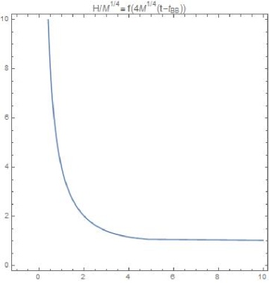
Figure 1: $H(t)$, implicitly defined in Eq.(29), as function of $(t-t_{\rm BB})$.

First, we notice from Eq.(29) that:

$$H(t)\to\infty\quad{\rm for}\;\;t-t_{\rm BB}\to 0\;,$$ (31)

in other words, there is a Big Bang at $t=t_{\rm BB}$ (30). Expanding the r.h.s. of Eq.(29) for small $(t-t_{\rm BB})$, equivalent to expanding for small $M$, yields:

$$t-t_{\rm BB}=\frac{1}{H}+\frac{M}{5H^{5}}+{\rm O}(M^{2})\;\;\longrightarrow\;\;$$

$$H(t)=\frac{1}{t-t_{\rm BB}}+\frac{M}{5}(t-t_{\rm BB})^{3}+{\rm O}(M^{2})\;.$$ (32)

The last relation in(32) implies a “coasting” [25] behavior of the universe for evolution times near the Big Bang. For the Friedmann scale factor itself we get from (32):

$$a(t)/a_{0}=(t-t_{\rm BB})\exp\bigl{\{}\frac{M}{20}(t-t_{\rm BB})^{4}+{\rm O}(M^{2})\bigr{\}}\;,$$ (33)

$${\rm i.e.}\;\;a(t)/a_{0}\simeq t-t_{\rm BB}\;\;{\rm for}\;{\rm small}\;(t-t_{\rm BB})\;,$$

in other words, close to the Big Bang the horizon $H^{-1}(t)$ and space $a(t)$ evolve in the same way.

On the other hand, for large $t$ (“late” universe):

$$H(t)\simeq M^{1/4}\quad,\quad\frac{\stackrel{{\scriptstyle..}}{{a}}}{a}\simeq\sqrt{M}=\frac{1}{3}\Lambda_{\rm DE}\;,$$ (34)

i.e., the universe evolves with a constant acceleration where $2\Lambda_{\rm DE}\equiv 6\sqrt{M}$ is the dark energy density.

3.2 Friedmann Scale Factor Solution for $M=0$

Let us consider the special case $M=0$, i.e., according to (15) $R_{\rm GB}^{2}$ dynamically vanishes. From Eq.(20) we have:

$$\stackrel{{\scriptstyle.}}{{H}}=-H^{2}\;\;\to\;\;H(t)=\frac{1}{t-t_{0}}\;\;\to\;\;a(t)/a_{0}=t-t_{0}\;,$$ (35)

which represent “coasting” universe’ evolution (linear expansion of the Friedmann scale factor) for all the time after the Big Bang at $t=t_{0}$.

Let us note that dynamical vanishing of $D=4$ Gauss-Bonnet scalar has been previously obtained in Ref. zanelli, however within a different and physically non-equivalent formalism - first-order (frame-bundle) formalism with a nonvanishing torsion.

3.3 Friedmann Scale Factor Solution for $M<0$

Now we consider the case $M<0$ (we will use the symbol ${\bar{M}}\equiv-M$ for convenience, i.e., according to (15) $R_{\rm GB}^{2}=-24{\bar{M}}<0$). Setting in the integral (28) $M=-{\bar{M}}$ we obtain the implicit solution for $H={\bar{H}}(t)$:

$$4\sqrt{2}{\bar{M}}^{1/4}(t-t_{0})=\log\Bigl{(}\frac{{\bar{H}}^{2}(t)+{\bar{M}}^{1/2}+\sqrt{2}{\bar{M}}^{1/4}{\bar{H}}(t)}{{\bar{H}}^{2}(t)+{\bar{M}}^{1/2}-\sqrt{2}{\bar{M}}^{1/4}{\bar{H}}(t)}\Bigr{)}$$

$$-2\arctan\Bigl{(}\frac{\sqrt{2}{\bar{H}}(t)}{{\bar{M}}^{1/4}}-1\Bigr{)}-2\arctan\Bigl{(}\frac{\sqrt{2}{\bar{H}}(t)}{{\bar{M}}^{1/4}}+1\Bigr{)}\;,\;\;\;$$ (36)

where the integration constant $t_{0}$ is defined by ${\bar{H}}(t=t_{0})=0$. From (36) we find both a Big Bang:

$${\bar{H}}(t)\to+\infty\;\;{\rm for}\;t=t_{\rm BB}\equiv t_{0}-\frac{\pi}{2\sqrt{2}{\bar{M}}^{1/4}}\;,$$ (37)

and a Big Crunch at finite cosmological times:

$${\bar{H}}(t)\to-\infty\;\;{\rm for}\;t=t_{\rm BC}\equiv t_{0}+\frac{\pi}{2\sqrt{2}{\bar{M}}^{1/4}}\;.$$ (38)

Similarly to the case $M>0$ (32)-(33) we obtain a “coasting” behaviour near the Big Bang ($(t-t_{\rm BB})$ small):

$${\bar{H}}(t)=\frac{1}{(t-t_{\rm BB})}-\frac{{\bar{M}}}{5}(t-t_{\rm BB})^{3}+{\rm O}({\bar{M}}^{2})\;,$$ (39)

$$a(t)/a_{0}=(t-t_{\rm BB})\exp\bigl{\{}-\frac{{\bar{M}}}{20}(t-t_{\rm BB})^{4}{\rm O}({\bar{M}}^{2})\bigr{\}}\;.$$ (40)

Near the Big Crunch ($(t_{\rm BC}-t)$ small) there is also a “coasting” behavior:

$${\bar{H}}(t)=-\frac{1}{(t_{\rm BC}-t)}+\frac{{\bar{M}}}{5}(t_{\rm BC}-t)^{3}+{\rm O}({\bar{M}}^{2})\;,$$ (41)

$$a(t)/a_{0}=(t_{\rm BC}-t)\exp\bigl{\{}-\frac{{\bar{M}}}{20}(t_{\rm BC}-t)^{4}+{\rm O}({\bar{M}}^{2})\bigr{\}}\;.$$ (42)

Here once again we observe that both near the Big Bang and near the Big Crunch the horizon and space sizes evolve in the same way.

4 Special Cosmological Solution of the full Gauss-Bonnet Gravity with a Dynamically Constant Gauss-Bonnet Scalar

We will now study in some detail special particular solutions of the extended Einstein Eqs.(11) (taking into account (15)) with a frozen composite field $\chi$ (10) ($\chi={\rm const}$):

$$R_{\mu\nu}-\frac{1}{2}g_{\mu\nu}R=\frac{1}{2}T_{\mu\nu}-12g_{\mu\nu}\chi M\quad,\quad R^{2}_{\rm GB}=24M\;.$$ (43)

Let us stress that we take the composite field $\chi\equiv\frac{\Phi(C)}{\sqrt{-g}}$ to be “frozen” to a constant as an additional condition after we derive the full system of equations of motion, including (11) and (14), from the original non-Riemannian volume-form action (6).

As we will see below, consistency of the system (43) will require the pertinent matter Lagrangian to be of a very specific form depending on the sign of the integration constant $M$.

We start by looking for cosmological solutions with $\chi={\rm const}$ of the Eqs.(21)-(22) – the FLRW reduction of (43). Inserting $\chi={\rm const}$ there we obtain:

$$6H^{2}-(\rho+24M\chi)=0\quad,\quad 6H^{2}+3(p-24M\chi)+\frac{12M}{H^{2}}=0$$ (44)

from which we deduce the equation of state:

$${\widetilde{\rho}}+3{\widetilde{p}}+\frac{72M}{{\widetilde{\rho}}}=0\quad,$$ (45)

$${\widetilde{\rho}}\equiv\rho+24M\chi\quad,\quad{\widetilde{p}}\equiv p-24M\chi\;,$$ (46)

where ${\widetilde{\rho}}$ and ${\widetilde{p}}$ are the shifted energy density and pressure incorporating the dynamically Gauss-Bonnet induced cosmological constant $\Lambda_{0}=12\chi M$ (16).

From the Friedmann Eqs.(21)-(22) we find:

$$\stackrel{{\scriptstyle.}}{{\phi}}^{2}=\rho+p=4\Bigl{(}H^{2}-\frac{M}{H^{2}}\Bigr{)}\;,$$ (47)

$$V(\phi)=\frac{1}{2}(\rho-p)=4H^{2}+2\frac{M}{H^{2}}-24M\chi\;,$$ (48)

$${\widetilde{V}}(\phi)\equiv V(\phi)+24M\chi=4H^{2}+2\frac{M}{H^{2}}\;,$$ (49)

where ${\widetilde{V}}(\phi)$ is the shifted scalar potential incorporating the dynamically Gauss-Bonnet induced cosmological constant $12M\chi$ (16).

4.1 Case $M>0$

Combining $\phi$-equations of motion (24) and the equation of state (45) yields a differential equation for ${\widetilde{\rho}}$ as function of the Friedmann scale factor $a$:

$$\frac{d{\widetilde{\rho}}}{da}=-\frac{2}{a}\Bigl{(}{\widetilde{\rho}}-\frac{36M}{{\widetilde{\rho}}}\Bigr{)}\quad\longrightarrow\quad{\widetilde{\rho}}(a)=\sqrt{36M+c_{0}a^{-4}}\;,$$ (50)

where $c_{0}$ is an integration constant. In accordance with the solution for the Friedmann scale factor in subsection 3.1, we obtain from (50):

• ${\widetilde{\rho}}(a)\simeq\sqrt{c_{0}}a^{-2}$ close to the Big Bang where $a\to 0$ – “coasting” behavior;

• ${\widetilde{\rho}}(a)\simeq 6\sqrt{M}$ in the late universe where $a\to\infty$ exponentially – $6\sqrt{M}$ is the dark energy density conforming to the late universe value of $H$ (34).

Relation (47) yields solution for $\phi(t)$ as function of $t$ through $H(t)$ as defined implicitly in (29):

$$\phi=2\int\frac{dH}{\sqrt{H^{2}-\frac{M}{H^{2}}}}\quad\longrightarrow$$

$$\phi(t)=\log\left(\sqrt{\frac{H^{4}(t)}{M}-1}+\frac{H^{2}(t)}{M^{1/2}}\right)$$ (51)

or, inversely, $H(t)$ as function of $\phi(t)$:

$$H^{2}=\sqrt{M}\cosh(\phi)\;.$$ (52)

The solution $\phi(t)$ (51) is graphically depicted in Fig.2.

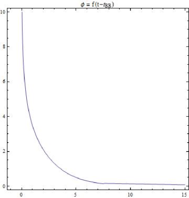
Figure 2: $\phi(t)$, defined in (51), as function of $(t-t_{\rm BB})$.

From (48) and (52) we find that the functional dependence of the scalar potential $V(\phi)$ or the shifted one ${\widetilde{V}}(\phi)$ (49) is uniquely fixed by the dynamics:

$${\widetilde{V}}(\phi)=4\sqrt{M}\cosh(\phi)+\frac{2\sqrt{M}}{\cosh(\phi)}\;.$$ (53)

From Eq.(51) for small $(t-t_{\rm BB})$ near the Big Bang (i.e., large $H$ according to (32)) we have:

$$\phi(t)\simeq 2\log H(t)\simeq-2\log(t-t_{\rm BB})\;.$$ (54)

On the other hand, in the “late” universe $\phi(t)$ (51) converges to zero – the minimum of the scalar potential (53), i.e., which yields precisely the value of the dark energy density:

$${\widetilde{V}}(\phi=0)=6\sqrt{M}\;.$$ (55)

4.2 Case $M=0$

For the purely “coasting” cosmology (subsection 3.2) from Eq.(51) (the integral on the first line) and from Eq.(48) we obtain when $M=0$:

$$\phi=2\log H=-2\log(t-t_{0})\quad,\quad V(\phi)=4e^{\phi}\;.$$ (56)

The equation of state (45) for $M=0$ becomes:

$$\rho+3p=0\;,$$ (57)

which is the same as, for instance, for the string gas [32].

4.3 Case $M<0$

Now, for the BigBang-BigCrunch cosmological solution (subsection 3.3), setting in the integral (51) $M=-{\bar{M}}<0$, we obtain the solution for $\phi(t)$ as function of ${\bar{H}}(t)$ (36):

$$\phi(t)=\log\left(\sqrt{\frac{{\bar{H}}^{4}(t)}{{\bar{M}}}+1}+\frac{{\bar{H}}^{2}(t)}{{\bar{M}}^{1/2}}\right)$$ (58)

or, inversely, ${\bar{H}}(t)$ as function of $\phi(t)$:

$${\bar{H}}^{2}=\sqrt{{\bar{M}}}\sinh(\phi)\;.$$ (59)

Accordingly, the functional dependence of the (shifted) scalar potential for $M=-{\bar{M}}<0$ is uniquely determined as:

$${\widetilde{V}}(\phi)=4\sqrt{{\bar{M}}}\sinh(\phi)+\frac{2\sqrt{{\bar{M}}}}{\sinh(\phi)}\;.$$ (60)

5 Discussion and Outlook

In the present paper we have made an essential use of the formalism of non-Riemannian spacetime volume-forms (alternative metric-independent volume elements, i.e., generally-covariant integration measure densities) defined in terms of auxiliary maximal rank tensor gauge fields, in order to construct a new type of Einstein-Gauss-Bonnet gravity in $D=4$ avoiding the need to couple the Gauss-Bonnet scalar to any matter fields. The presence of the non-Riemannian volume element in the $D=4$ Gauss-Bonnet action terms makes the theory non-trivial and well-defined. The principal new feature is that on-shell the Gauss-Bonnet scalar becomes an arbitrary integration constant. In the cosmological setting the dynamical constancy of the Gauss-Bonnet scalar by itself completely determines the solutions for the Hubble parameter $H(t)$ and the Friedmann scale factor $a(t)$ as functions of the cosmological time without any influence of the matter dynamics (no back reaction of matter on the cosmological metric).

The whole effect of matter on the spacetime is absorbed by the time-dependence of the composite field $\chi$ (10) (the ratio of the non-Riemannian volume element $\Phi(C)$ to the standard Riemannian $\sqrt{-g}$). If we choose to “freeze” $\chi={\rm const}$, then in the case of scalar field matter the scalar potential $V(\phi)$ is uniquely constrained to be of a very specific form as a function of $\phi$.

The solutions for $H(t)$ and $a(t)$ between “coasting” early Big Bang cosmology, where the evoluton of $a(t)$ coincides with the evolution of the horizon ($H^{-1}(t)$), and a late time de Sitter universe ($M>0$) or a Big Crunch ($M<0$) at a finite cosmological time, depend on the sign of the dynamically generated constant value $M$ of the Gauss-Bonnet scalar. The case $M>0$ is more realistic, but still too simplified to be realistic enough to describe the whole evolution of the observed universe, since it predicts continuous acceleration during the whole evolution.

Thus, our $D=4$ Einstein-Gauss-Bonnet model could be considered as an approximation to be used in the future as a basis for a more realistic cosmological models. For example, a model like ours could be an interesting candidate for the high-energy limit of a realistic model. This is because of the property of the composite field $\chi=\Phi(C)/\sqrt{-g}$ to absorb the effects of a non-trivial matter behaviour and to prevent a matter back reaction on the spacetime metrics. Such an effect could be exactly what is needed to cure the issues noticed in Ref. afshordi, where it has been shown that quantum fluctuations in the energy-momentum tensor of matter can cause serious phenomenological problems. The latter could however be avoided provided at high energies exists a field like $\chi$ that compensates the effects of the matter fluctuations.

Still, we can slightly generalize our $D=4$ Einstein-Gauss-Bonnet model (6) to yield more realistic cosmological solutions, namely, to provide continuous acceleration during the early universe epoch after the Big Bang as well as during the late universe (dark energy) epoch, while providing deceleration for an intermediate epoch.

To this end we can consider the more general (than (6)) action:

$$S=\int d^{4}x\sqrt{-g}\Bigl{[}R-\frac{1}{2}g^{\mu\nu}\partial_{\mu}\phi\partial_{\nu}\phi-V(\phi)\Bigr{]}$$

$$+\int d^{4}x\,\Phi(C)\,\Bigl{(}R_{\rm GB}^{2}-24W(\phi)\Bigr{)}\;,$$ (61)

with an additional appropriately chosen scalar potential term $W(\phi)$ (the factor $24$ is introduced for numerical convenience).

Now, instead of (15) the equations of motion w.r.t. auxiliary tensor gauge field $C_{\mu\nu\lambda}$ defining the non-Riemannian volume element $\Phi(C)$ yield:

$$\partial_{\mu}\Bigl{(}R_{\rm GB}^{2}-24W(\phi)\Bigr{)}=0\quad\longrightarrow\quad R_{\rm GB}^{2}=24\bigl{(}M+W(\phi)\bigr{)}={\rm const}\;,$$ (62)

where again $M$ is an arbitrary integration constant and will be absorved into $W(\phi)$, henceforth $W(\phi)+M\equiv{\widetilde{W}}(\phi)$.

In the cosmological FLRW reduction Eq.(62) yields instead of (20):

$$\stackrel{{\scriptstyle.}}{{H}}=-H^{2}+\frac{{\widetilde{W}}(\phi)}{H^{2}}\quad,\quad\frac{\stackrel{{\scriptstyle..}}{{a}}}{a}=\frac{{\widetilde{W}}(\phi)}{H^{2}}\;,$$ (63)

so that now we can have both acceleration or deceleration.

Indeed, now upon setting as above the composite field $\chi={\rm const}$ the Friedman equations and the equation of state, as well as the equations for $\stackrel{{\scriptstyle.}}{{\phi}}^{2}$ and the initial scalar potential $V(\phi)$ retain the same form as in (44)-(46) and (47)-(49), respectively, with replacing there $M\longrightarrow{\widetilde{W}}(\phi)$, in particular:

$$\stackrel{{\scriptstyle.}}{{\phi}}=-2\sqrt{H^{2}-\frac{{\widetilde{W}}(\phi)}{H^{2}}}\quad,\quad({\rm or,~{}equivalently})\;\;\frac{dH}{d\phi}=\frac{1}{2}\sqrt{H^{2}-\frac{{\widetilde{W}}(\phi)}{H^{2}}}\;,$$ (64)

$$V(\phi)+24\chi{\widetilde{W}}(\phi)=4H^{2}+2\frac{{\widetilde{W}}(\phi)}{H^{2}}\;.$$ (65)

The explicit functional dependence of $V(\phi)$ on $\phi$ is uniquely fixed by Eq.(65) in terms of the given ${\widetilde{W}}(\phi)$ (Fig.3 below) upon substituting there the solution $H=H(\phi)$ of the second Eq.(64).

Let us now choose ${\widetilde{W}}(\phi)$ of the form qualitatively depicted on Fig.3.

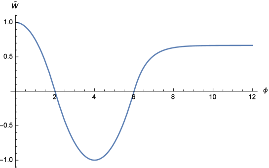
Figure 3: Qualitative shape of ${\widetilde{W}}(\phi)$.

Since ${\widetilde{W}}(\phi)$ quickly approaches its asymptotic value ${\widetilde{W}}(\infty)>0$ for large $\phi$, Eqs.(63)-(64) will have approximate solutions as in (29),(51) where $M$ is replaced by ${\widetilde{W}}(\infty)$, i.e., again we will have Big Bang at $t_{\rm BB}\simeq t_{0}-\frac{\pi}{4\bigl{(}{\widetilde{W}}(\infty)\bigr{)}^{1/4}}$. On the other hand, for late times from (63)-(65) we obtain:

$$H(t\to\infty)\simeq\bigl{(}{\widetilde{W}}(0)\bigr{)}^{1/4}\quad,\quad\phi(t\to\infty)\simeq 0\;,$$ (66)

$$V(0)+24\chi{\widetilde{W}}(0)=6\sqrt{{\widetilde{W}}(0)}={\rm dark~{}energy~{}density}\;.$$ (67)

In a subsequent study we will explore more systematically the more realistic Einstein-Gauss-Bonnet model (61) which should involve numerical treatment of the nonlinear system of equations (63)-(64).

References

- [1] S. Capozziello and M. De Laurentis, Phys. Reports 509, 167 (2011) (arXiv:1108.6266).
- [2] S. Capozziello and V. Faraoni, “Beyond Einstein Gravity – A Survey of Gravitational Theories for Cosmology and Astrophysics”, (Springer, 2011).
- [3] S. Nojiri and S. Odintsov, Phys. Reports 505, 59 (2011).
- [4] S. Nojiri, S. Odintsov and V. Oikonomou, Phys. Reports 692, 1 (2017) (arXiv:1705.11098).
- [5] E. Guendelman, E. Nissimov and S. Pacheva, Eur. J. Phys. C75, 472-479 (2015) (arXiv:1508.02008); Eur. J. Phys. C76, 90 (2016) (arXiv:1511.07071).
- [6] E. Guendelman, E. Nissimov and S. Pacheva, Int. J. Mod. Phys. D25, 1644008 (2016) (arXiv:1603.06231).
- [7] E. Guendelman, E. Nissimov and S. Pacheva, in “Quantum Theory and Symmetries with Lie Theory and Its Applications in Physics”, vol.2 ed. V. Dobrev, Springer Proceedings in Mathematics and Statistics v.225 (Springer, 2018).
- [8] E. Guendelman, E. Nissimov and S. Pacheva, arXiv:1808.03640, to be published in 10th Jubilee Conference of Balkan Physical Union, AIP Conference Proceedings.
- [9] E. Guendelman, E. Nissimov and S. Pacheva, Bulg. J. Phys. 41, 123 (2014) (arXiv:1404.4733).
- [10] E. Guendelman, E. Nissimov and S. Pacheva, Int. J. Mod. Phys. A30, 1550133 (2015) (arXiv:1504.01031).
- [11] E. Guendelman, Mod. Phys. Lett. A14 1043-1052 (1999) (arXiv:gr-qc/9901017).
- [12] E. Guendelman and A. Kaganovich, Phys. Rev. D60 065004 (1999) (arXiv:gr-qc/9905029).
- [13] E. Berti, E. Barausse, V. Cardoso et al., Class. Quantum Grav. 32, 243001 (2015) (arXiv:1501.07274).
- [14] L. Barack, V. Cardoso, S. Nissanke et al., arXiv:1806.05195, to appear in Class. Quant. Grav. (2018).
- [15] S. Nojiri and S. D. Odintsov, Phys. Lett. B631, 1 (2005) (hep-th/0508049).
- [16] S. Nojiri, S.D. Odintsov and O.G. Gorbunova, J. Physics A39, 6627 (2006) (arXiv:hep-th/0510183).
- [17] G. Cognola, E. Elizalde, S. Nojiri, S.D. Odintsov and S. Zerbini, Phys. Rev. D73, 084007 (2006) (arXiv:hep-th/0601008).
- [18] A. De Felice and S. Tsujikawa, Phys. Lett. B675, 1 (2009) (arXiv:0810.5712).
- [19] P.Kanti, R.Gannouji and N. Dadhich (2015) Phys. Rev. D92, 041302 (2015) (arXiv:1503.01579); Phys. Rev. D92, 083524 (2015) (arXiv:1506.04667).
- [20] L. Sberna and P. Pani, Phys. Rev. D96, 124022 (2017) (arXiv:170806371).
- [21] M. Heydari-Fard, H. Razmi and M. Yousefi, Int. J. Mod. Phys. D26, 1750008 (2017).
- [22] S.Carloni and J.Mimoso Eur. Phys. J. C77, 547 (2017).
- [23] M. Benetti, S. Santos da Costa, S. Capozziello, J. S. Alcaniz and M. De Laurentis, Int. J. Mod. Phys. D27, 1850084 (2018) (arXiv:1803.00895.
- [24] S.Odintsov, V.Oikonomou and S. Banerjee, arXiv:1807.00335.
- [25] E.W. Kolb, Astrophys. J. 344, 543-550 (1989).
- [26] K. Gediz Akdeniz, A. Metin and E. Rizaoglu, Phys. Lett. 321B, 329-332 (1994).
- [27] P. Singh and D. Lohiya, JCAP 1505, 061 (2015) (arXiv:1312.7706).
- [28] G. Singh and D. Lohiya, Mon. Not. Roy. Astron. Soc., 473,14-19 (2018).
- [29] R. Myrzakulov, L. Sebastiani and S. Zerbini, Gen. Rel. Gravit. 45, 675 (2013) (arXiv:1208.3392).
- [30] P. Bargue and E. Vagenas, Eur. Phys. Lett. 115, 60002 (2016) (arXiv:1609.07933).
- [31] I. Radinschi, T. Grammenos, F. Rahaman, A. Spanou, M. Cazacu, S. Chattapadhyay and A. Pasqua, arXiv:1807.00300.
- [32] A. Vilenkin, Phys. Rev. D24, 2082 (1981)
- [33] A. Toloza and J. Zanelli, Class. Quantum Grav. 30, 135003 (2013) (arXiv:1301.0821).
- [34] N. Afshordi and E. Nelson, Phys. Rev. D93, 083505 (2016) (arXiv:1504.00012).