Spin correlations of quantum-spin-liquid and quadrupole-ordered states of Tb_2+xTi_2-xO_7+y

Abstract

Spin correlations of the frustrated pyrochlore oxide Tb_2+xTi_2-xO_7+y have been investigated by using inelastic neutron scattering on single crystalline samples ($x=-0.007,0.000,$ and $0.003$), which have the putative quantum-spin-liquid (QSL) or electric-quadrupolar ground states. Spin correlations, which are notably observed in nominally elastic scattering, show short-ranged correlations around $L$ points [$\bm{q}=(\tfrac{1}{2},\tfrac{1}{2},\tfrac{1}{2})$], tiny antiferromagnetic Bragg scattering at $L$ and $\Gamma$ points, and pinch-point type structures around $\Gamma$ points. The short-ranged spin correlations were analyzed using a random phase approximation (RPA) assuming the paramagnetic state and two-spin interactions among Ising spins. These analyses have shown that the RPA scattering intensity well reproduces the experimental data using temperature and $x$ dependent coupling constants of up to 10 neighbor site pairs. This suggests that no symmetry breaking occurs in the QSL sample, and that a quantum treatment beyond the semi-classical RPA approach is required. Implications of the experimental data and the RPA analyses are discussed.

I Introduction

Geometrically frustrated magnets archetypally on the two-dimensional (2D) triangle Wannier (1950) and kagomé Syôzi (1951); Qi et al. (2008) lattices, and on the three-dimensional (3D) pyrochlore lattice Gardner et al. (2010) have been actively studied for decades Lacroix et al. (2011). Among classical frustrated magnets, spin ice Bramwell and Gingras (2001) has been extensively studied from many viewpoints, e.g., macroscopically degenerate ground states Ramirez et al. (1999), partial lifting of the degeneracy under magnetic field Matsuhira et al. (2002), and fractionalized excitations Castelnovo et al. (2008); Kadowaki et al. (2009). Quantum effects in frustrated magnetic systems ranging from quantum annealing Kadowaki and Nishimori (1998); King et al. (2018) to quantum spin liquid (QSL) states Savary and Balents (2017), the origin of which dates back to the proposal of the RVB state Anderson (1973), have attracted much attention. Experimental challenges of finding real QSL substances Hirakawa et al. (1985); Gardner et al. (1999) and of investigating QSL states using available techniques Han et al. (2012); Ross et al. (2011); Chang et al. (2012); Shen et al. (2016); Fåk et al. (2017); Sibille et al. (2018) have been addressed in recent years.

Among frustrated magnetic pyrochlore oxides Gardner et al. (2010) a non-Kramers pyrochlore magnet Tb_2+xTi_2-xO_7+y (TTO) Kadowaki et al. (2018) has been investigated for decades as a QSL candidate, since conventional magnetic order has not been observed in any experiments under zero field and zero static pressure Gardner et al. (1999, 2010). On the basis of theoretical insight that TTO is not much different from classical spin ice, the phrase quantum spin ice (QSI) was coined for the QSL state of TTO Molavian et al. (2007); Gingras and McClarty (2014). However, its nature has remained elusive. Recently we showed that this putative QSL state is limited in a range of the small off-stoichiometry parameter $x<x_{\text{c}}\simeq-0.0025$ Taniguchi et al. (2013); Wakita et al. (2016); Kadowaki et al. (2018). In the other range $x_{\text{c}}<x$, we showed that TTO undergoes a phase transition most likely to an electric multipolar [or quadrupole ordered (QO)] state ($T<T_{\text{c}}$) Takatsu et al. (2016a, b); Kadowaki et al. (2018), which is described by a pseudospin-$\frac{1}{2}$ Hamiltonian modified from the classical spin ice to a quantum model by adding transverse pseudospin terms Onoda and Tanaka (2011). The estimated parameter set of this Hamiltonian Takatsu et al. (2016a) is close to the theoretical phase boundary between the electric quadrupolar state and a U(1) QSL state (QSI) Lee et al. (2012); Hermele et al. (2004), which is thereby a theoretical QSL candidate for TTO. At present, few researchers have addressed the problem of the QSL state of TTO using well $x$-controlled samples.

Previous neutron scattering experiments on TTO, which were performed on samples with unknown and known $x$, showed that spin correlations, defined by the wavevector dependence of scattering intensity are most clearly seen in energy-resolution-limited (nominally) elastic scattering at low temperatures. In the observed spin correlations there are three important features: magnetic short-range order (SRO) with the wavevector $\bm{q}=(\tfrac{1}{2},\tfrac{1}{2},\tfrac{1}{2})$ ($L$ point of the first Brillouin zone of the FCC lattice) Yasui et al. (2002); Fennell et al. (2012); Petit et al. (2012); Fritsch et al. (2013), pinch point structures around $\bm{q}=0$ ($\Gamma$ point) Fennell et al. (2012); Petit et al. (2012), and tiny antiferromagnetic Bragg reflections at $L$ and $\Gamma$ points Taniguchi et al. (2013); Takatsu et al. (2016a). It should be noted that details of the observed scattering intensities in these studies depended on samples (on $x$). This may intriguingly suggest that the ground states of TTO are potentially highly degenerate and they are lifted in various ways depending on slight differences of samples.

Very recently we performed inelastic neutron scattering (INS) experiments on $x$-controlled TTO single-crystalline samples with $x=-0.007<x_{\text{c}}$ (QSL) and $x_{\text{c}}<x=0.000,0.003$ (QO) Kadowaki et al. (2018). In this paper we focus on the $\bm{q}=(\tfrac{1}{2},\tfrac{1}{2},\tfrac{1}{2})$ SRO of these samples and perform quantitative analyses in order to shed light on how these spin correlations reflect the QSL state. In previous investigations Fritsch et al. (2013); Guitteny et al. (2015), analyses of the $\bm{q}=(\tfrac{1}{2},\tfrac{1}{2},\tfrac{1}{2})$ SRO were carried out by assuming that there exist static short-ranged classical spins with cluster sizes of the order 10 Å. However no clusters which adequately reproduce the observed intensity pattern were found, although a few clusters showing limited goodness-of-fit were obtained Fritsch et al. (2013); Guitteny et al. (2015). This failure indicates either that the samples were not well controlled or that the analysis methods they used are not sufficiently systematic.

The first problem of controlling the composition of the samples is resolved in the present study. In contrast, the second problem can originate from a profound property of the QSL state, and will be resolved only by analyses reflecting the quantum nature of the many-body ground state. However, since no practical quantum model calculations are available at present, in the present study, we attempt to apply a systematic but still semi-classical approach using a random phase approximation (RPA) Jensen and Mackintosh (1991). This would lead us to a reasonable result if the SRO could be interpreted within the classical spin paradigm, or leads us to a certain paradoxical result if it essentially contains many-body quantum effects.

II Methods

II.1 Experimental Methods

Single crystalline samples of Tb_2+xTi_2-xO_7+y with $x=-0.007,0.000$ and $0.003$ used in this study are those of Ref. Kadowaki et al. (2018), where methods of the sample preparation and the estimation of $x$ are described. The QSL sample with $x=-0.007$ remains in the paramagnetic state down to 0.1 K. The QO samples with $x=0.000$ and $x=0.003$ very likely have small and large electric quadrupole orders, respectively, at $T\ll T_{c}\sim 0.4$ K Taniguchi et al. (2013); Wakita et al. (2016). We note that the values of $x$ among different investigation groups are not necessarily consistent Kadowaki et al. (2018), and that our $x$ values of the samples used in Refs. Taniguchi et al. (2013); Kadowaki et al. (2015); Takatsu et al. (2016a, b); Wakita et al. (2016); Takatsu et al. (2017); Kadowaki et al. (2018) are self-consistent.

Neutron scattering experiments were carried out on the time-of-flight (TOF) spectrometer IN5 Fak (a, b) operated with $\lambda=8$ Å at ILL for the $x=-0.007$ and 0.000 crystal samples. The energy resolution of this condition was $\Delta E=0.021$ meV (FWHM) at the elastic position. Neutron scattering experiments for the $x=0.003$ crystal sample were performed on the TOF spectrometer AMATERAS operated with $\lambda=7$ Å at J-PARC. The energy resolution of this condition was $\Delta E=0.024$ meV (FWHM) at the elastic position. Each crystal sample was mounted in a dilution refrigerator so as to coincide its $(h,h,l)$ plane with the horizontal scattering plane of the spectrometer. The observed intensity data were corrected for background and absorption using a home-made program Kadowaki (a). Construction of four dimensional $S(\bm{Q},E)$ data object from a set of the TOF data taken by rotating each crystal sample was performed using HORACE Ewings et al. (2016).

To analyze the $\bm{Q}$-dependence of the (nominally) elastic scattering intensity (Fig. 1 in Ref. Kadowaki et al. (2018)), we integrated $S(\bm{Q},E)$ in a small energy range $-\epsilon<E<\epsilon$. We chose $\epsilon=0.025$ and $0.030$ meV for IN5 and AMATERAS data, respectively, which are a little larger than the instrumental resolutions. These 3D data sets $[S(\bm{Q})]_{\text{el}}=\int_{-\epsilon}^{\epsilon}S(\bm{Q},E)dE$ are normalized by the method described in Ref. Kadowaki et al. (2018), i.e., using the “arb. units” of Fig. 1 in Ref. Kadowaki et al. (2018). Consequently the elastic intensities can be compared mutually among the three samples.

II.2 RPA model calculation

The RPA model calculation of $S(\bm{Q},E)$ using the pseudospin-$\frac{1}{2}$ Hamiltonian appropriate for quadrupole ordered phases is described in Ref. Kadowaki et al. (2015). We used a similar RPA method to calculate the elastic scattering intensity $[S(\bm{Q})]_{\text{el}}$ assuming that the system is in the paramagnetic phase. This assumption is made because we are interested mainly in the low-temperature QSL and the high-temperature paramagnetic states. Details and related definitions are described in Appendix A.

For the sake of simplicity we consider a pseudospin-$\frac{1}{2}$ Hamiltonian which is decoupled between magnetic dipole ($\sigma_{\bm{r}}^{z}$) and electric quadrupole ($\sigma_{\bm{r}}^{x}$ and $\sigma_{\bm{r}}^{y}$) terms, the latter of which can be neglected for the present purpose. We adopt a magnetic Hamiltonian expressed by

$$H_{\text{m}}=\sum_{m}J_{m}\left\{\sum_{\langle{\bm{r}},{\bm{r}}^{\prime}\rangle_{m}}\sigma_{\bm{r}}^{z}\sigma_{\bm{r}^{\prime}}^{z}\right\}+Dr_{\text{nn}}^{3}$$ (1)

$$\times \sum_{\langle\bm{r},\bm{r}^{\prime}\rangle}\left\{\frac{\bm{z}_{{\bm{r}}}\cdot\bm{z}_{{\bm{r}}^{\prime}}}{|\Delta\bm{r}|^{3}}-\frac{3[\bm{z}_{{\bm{r}}}\cdot\Delta\bm{r}][\bm{z}_{{\bm{r}}^{\prime}}\cdot\Delta\bm{r}]}{|\Delta\bm{r}|^{5}}\right\}\sigma_{\bm{r}}^{z}\sigma_{\bm{r}^{\prime}}^{z}\;,$$

which is an expansion of that of Refs. Kadowaki et al. (2015); Takatsu et al. (2016a). The first term of Eq. (1) stands for magnetic coupling allowed by the space group symmetry between the Ising spin operators. The summation runs over coupling constants $J_{m}$ ($m=1,\cdots,m_{\text{max}}$, $m_{\text{max}}\leq 16$) and corresponding site pairs $\langle{\bm{r}},{\bm{r}}^{\prime}\rangle_{m}$. These site pairs are listed in Table 3. The nearest-neighbor (NN) coupling constant $J_{1}$ is usually expressed as $J_{\text{nn}}$ for the NN spin ice model ($J_{\text{nn}}=J_{1}>0$). The other couplings as far as 10 neighbor site pairs had to be included to obtain good fit of the experimental data. Since the coupling constants beyond third-neighbor site pairs ($J_{m>4}$) are probably much smaller than $J_{1}$, they would be effective values or experimental parameters. The second term of Eq. (1) represents the classical dipolar interaction den Hertog and Gingras (2000), where $r_{\text{nn}}$ is the NN distance and $\Delta\bm{r}=\bm{r}-\bm{r}^{\prime}$. The parameter $D$ is determined by the magnitude of the magnetic moment of the crystal field ground state doublet. We adopt $D=0.29$ K, corresponding to the magnetic moment 4.6 $\mu_{\text{B}}$ Takatsu et al. (2016a).

The generalized susceptibility $\chi_{\nu,\nu^{\prime}}(\bm{k},E=0)$ is computed by solving Eq. (6) with $E=0$, i.e.,

$$\sum_{\nu^{\prime\prime}}[\delta_{\nu,\nu^{\prime\prime}}-\chi_{\text{L}}J_{\nu,\nu^{\prime\prime}}(\bm{k})]\chi_{\nu^{\prime\prime},\nu^{\prime}}(\bm{k},0)=\delta_{\nu,\nu^{\prime}}\chi_{\text{L}}\;,$$ (2)

where $J_{\nu,\nu^{\prime}}(\bm{k})$ denotes the Fourier transform of the magnetic coupling constants [Eq. (7)] and $\chi_{\text{L}}$ is the local susceptibility [Eq. (8)]. Using $\chi_{\nu,\nu^{\prime}}(\bm{k},0)$, the elastic scattering $[S(\bm{Q})]_{\text{el}}$ is given by

$$[S(\bm{Q} = \bm{G}+\bm{k})]_{\text{el}}\propto f(Q)^{2}\sum_{\rho,\sigma,\nu,\nu^{\prime}}(\delta_{\rho,\sigma}-\hat{Q}_{\rho}\hat{Q}_{\sigma})$$ (3)

$$\times U_{\rho,z}^{(\nu)}U_{\sigma,z}^{(\nu^{\prime})}\chi_{\nu,\nu^{\prime}}(\bm{k},0)\cos[\bm{G}\cdot(\bm{d}_{\nu}-\bm{d}_{\nu^{\prime}})]\>,$$

where $f(Q)$ is the form factor of Tb³⁺, in the quasi-elastic approximation [Eq. (10)].

III Results

III.1 QSL sample with $x=-0.007$

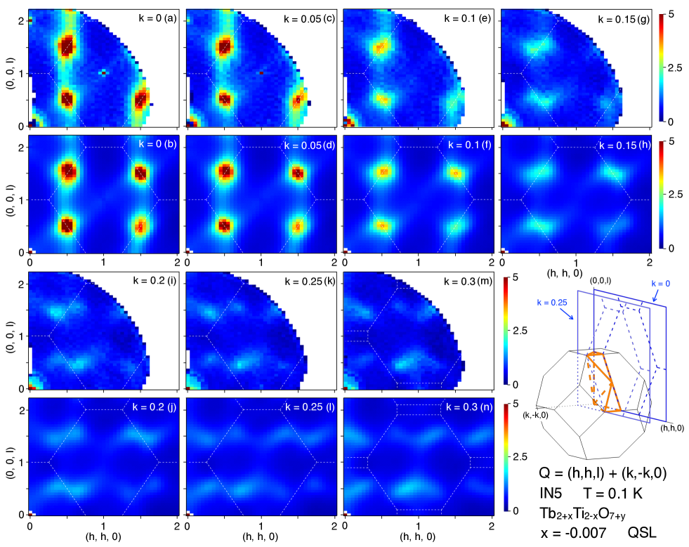
Figure 1: Intensity maps of 3D data $[S(\bm{Q})]_{\text{el}}$ taken at 0.1 K for the QSL sample with $x=-0.007$. The 3D data are viewed by 2D slices (a,c,e,g,i,k,m), which are parallel cross-sections of $\bm{Q}=(h,h,l)+(k,-k,0)$ with fixed $k$. These can be compared to the typical RPA $[S(\bm{Q})]_{\text{el}}$ (b,d,f,h,j,l,n) obtained by least squares fit using the 13 coupling constants, $J_{1},\cdots,J_{13}$, listed in Table 1. Dashed lines in these 2D slices (a-n) are boundaries of Brillouin zones. The bottom right corner shows the first Brillouin zone of the FCC lattice (thin black lines), irreducible zone (thick orange lines), and two 2D slice planes labeled $k=0$ and $0.25$ (blue lines).

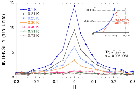
Figure 2: Temperature dependence of intensity $[S(\bm{Q})]_{\text{el}}$ along a trajectory through $\bm{Q}=(\tfrac{1}{2},\tfrac{1}{2},\tfrac{1}{2})$, which was measured by fixing the sample rotation angle. The abscissa of this figure is a projection of the $\bm{Q}$ trajectory (blue line in inset) to a straight line $\bm{Q}=(1/2,1/2,1/2)+(H/2,H/2,H)$ (red dashed line in inset).

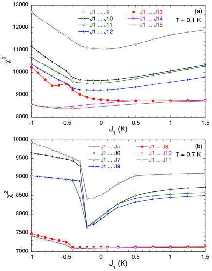
Figure 3: Minimized values of the weighted sum of squared residuals $\chi^{2}$ as a function of the fixed parameter $J_{1}$. (a) Results of least squares fits of $[S(\bm{Q})]_{\text{el}}$ with adjustable parameters $J_{m}$ ($m\leq m_{\text{max}}=9,\cdots,15$) for the QSL sample with $x=-0.007$ taken at $0.1$ K (Fig. 1). The number of fit data is 10185. (b) Results of least squares fits of $[S(\bm{Q})]_{\text{el}}$ with adjustable parameters $J_{m}$ ($m\leq m_{\text{max}}=5,\cdots,11$) for the QSL sample with $x=-0.007$ taken at $0.7$ K (Fig. 4). The number of fit data is 10147.

Table 1: Typical coupling constants $J_{m}$ (in units of K) of Eq. (1) obtained by least squares fits of observed 3D data sets $[S(\bm{Q})]_{\text{el}}$ to Eq. (3). The calculated $[S(\bm{Q})]_{\text{el}}$ using these $J_{m}$ are shown in Fig. 1 ($x=-0.007$, $T=0.1$ K), Fig. 4 ($x=-0.007$, $T=0.7$ K), Fig. 5 ($x=0.000$, $T=0.1$ K), Fig. 6 ($x=0.000$, $T=0.7$ K), and Fig. 8 ($x=0.003$, $T=0.1$ K). Numerical uncertainty of $J_{m}$ is discussed in Appendix B and Ref. Sup .

3D data	$J_{1}$	$J_{2}$	$J_{3}$	$J_{4}$	$J_{5}$	$J_{6}$	$J_{7}$	$J_{8}$	$J_{9}$	$J_{10}$	$J_{11}$	$J_{12}$	$J_{13}$	$J_{14}$
Fig. 1	1.0	0.824	1.011	0.176	0.184	0.410	0.436	0.355	1.060	-0.026	-0.066	-0.071	0.378
Fig. 4	1.0	0.070	0.536	-0.373	-0.370	0.076	-0.007	-0.020	0.919
Fig. 5	1.0	0.836	1.191	0.102	0.109	0.487	0.745	0.574	1.732	0.037	0.014	-0.137	0.464
Fig. 6	1.0	-0.101	0.751	-0.501	-0.408	0.191	0.078	-0.019	1.364
Fig. 8	0.25	-0.279	-0.040	-0.237	-0.081	-0.124	0.297	0.022	0.098	-0.061	-0.031	-0.060	-0.119	0.191

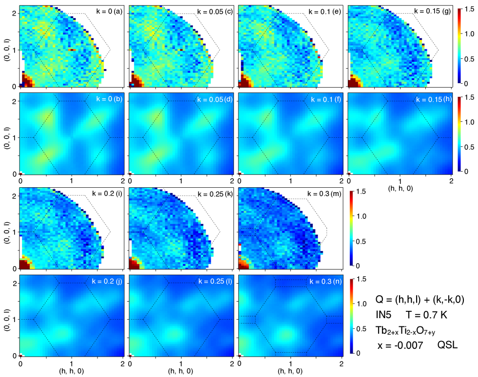
Figure 4: Intensity maps of 3D data $[S(\bm{Q})]_{\text{el}}$ taken at 0.7 K for the QSL sample with $x=-0.007$. The 3D data are viewed by 2D slices (a,c,e,g,i,k,m), which are parallel cross-sections of $\bm{Q}=(h,h,l)+(k,-k,0)$ with fixed $k$. These can be compared to the typical RPA $[S(\bm{Q})]_{\text{el}}$ (b,d,f,h,j,l,n) obtained by least squares fit using the 9 coupling constants, $J_{1},\cdots,J_{9}$, listed in Table 1. Dashed lines in these 2D slices (a-n) are boundaries of Brillouin zones.

Figure 1(a,c,e,g,i,k,m) shows a 3D data set $[S(\bm{Q})]_{\text{el}}$ taken at 0.1 K for the QSL sample with $x=-0.007$. These 3D data are shown by seven 2D slices of $\bm{Q}=(h,h,l)+(k,-k,0)$ with fixed $k$ values. Two slice planes with $k=0$ and 0.25 are illustrated at the bottom right corner of Fig. 1 with the first Brillouin zone of the FCC lattice and an irreducible zone. From this figure one can see that the observed $\bm{Q}$-range encompasses an independent part of the first Brillouin zone, which is an advantage over the previous experiments, which is limited to the 2D slice with $k=0$ Yasui et al. (2002); Fennell et al. (2012); Petit et al. (2012); Fritsch et al. (2013).

The observed 3D data $[S(\bm{Q})]_{\text{el}}$ of Fig. 1 show two features: strong short-ranged spin correlations with wavevector $\bm{q}=(\tfrac{1}{2},\tfrac{1}{2},\tfrac{1}{2})$, and very weak pinch-point structures around $\bm{Q}=(1,1,1)$ and $(0,0,2)$. By comparing the 2D slice of Fig. 1(a) with those of the previous investigations Yasui et al. (2002); Fennell et al. (2012); Petit et al. (2012); Fritsch et al. (2013), one can see both differences and similarities among the investigations. This fact confirms the importance of controlling the $x$ value for quantitative studies.

In order to measure the temperature dependence of the $\bm{q}=(\tfrac{1}{2},\tfrac{1}{2},\tfrac{1}{2})$ SRO we measured intensities along a trajectory through $\bm{Q}=(\tfrac{1}{2},\tfrac{1}{2},\tfrac{1}{2})$ by fixing the sample rotation angle. The resulting temperature dependence of $[S(\bm{Q})]_{\text{el}}$ is plotted in Fig. 2. As temperature is decreased below 0.4 K, the spin correlations grow continuously without a phase transition. We estimate the correlation length $\xi$ from the half width at half maximum (HWHM) of the peak ($1/\xi$ = HWHM). It increases to $\xi\sim 20$ Å at 0.1 K. This correlation length and the temperature scale of 0.4 K agree with those reported in Ref. Guitteny et al. (2015), where powder samples were used (Fig. 3(b) in Ref. Guitteny et al. (2015)). We note that the correlation length reported in Ref. Fritsch et al. (2013), where a single crystal sample was used, is significantly shorter ($\sim 8$ Å).

An important point concerning the discrepancy of the correlation length noted above concerns the thermal response time of the system. In particular, we observed very slow cooling of the sample especially below 0.4 K in the present experimental condition. More specifically, it took about two days for the scattering intensity to become time independent after cooling the mixing chamber down to 0.1 K. This slow cooling is ascribable to very low thermal conductivity of TTO Li et al. (2013) and the large size of the crystal sample for INS. One has to carefully distinguish this long relaxation time to other interpretations, for example, the cooling protocol dependence reported in Ref. Kermarrec et al. (2015), where the authors might not have waited enough time, which may possibly result in a short correlation length.

We performed least squares fits of the observed 3D data set $[S(\bm{Q})]_{\text{el}}$ to the RPA intensity Eq. (3). Adjustable parameters are the coupling constants $J_{m}$ ($1\leq m\leq m_{\text{max}}$), the local susceptibility $\chi_{\text{L}}$, and an intensity scale factor. After several trial computations, we became aware of a problem that these parameters cannot be independently adjusted. To avoid this problem and exclude unrealistic solutions, we fixed $J_{1}$ and imposed a restriction on $J_{m}$ ($2\leq m\leq m_{\text{max}}$) by adding a penalty function $\sum_{2\leq m\leq m_{\text{max}}}\left(\tfrac{J_{m}}{1\text{ K}}\right)^{8}$ to the weighted sum of squared residuals

$$\chi^{2}=\sum_{i=1}^{N}\left(\tfrac{\text{obs}(i)-\text{calc}(i)}{\text{error}(i)}\right)^{2}\>,$$ (4)

where $N=10185$ is the number of intensity data used in the fitting. Technical details of the least squares fits are discussed in Appendix B and Ref. Sup .

In Fig. 3(a) we plot minimized values of $\chi^{2}$ as a function of fixed $J_{1}$ (detailed discussion on inspecting the least squares fits is given in Ref. Sup ). As $J_{1}$ is decreased in the range $J_{1}<-5D/3$, which favors the antiferromagnetic “all-in–all-out” LRO for $J_{m>1}=0$ den Hertog and Gingras (2000), the fits become unsatisfactory. These plots also show that the inclusion of further coupling constants $J_{m}$ with $m_{\text{max}}\geq 14$ does not improve the fitting.

By inspecting 3D data $[S(\bm{Q})]_{\text{el}}$ calculated using several sets of fitted parameters, we chose a typical good result of the fitting. This typical $[S(\bm{Q})]_{\text{el}}$ is shown in Fig. 1(b,d,f,h,j,l,n), which is calculated using the values of $J_{1},\cdots,J_{13}$ listed in Table 1. One can see that the RPA model calculation excellently reproduces the observed $[S(\bm{Q})]_{\text{el}}$. Almost the same features of the $\bm{q}=(\tfrac{1}{2},\tfrac{1}{2},\tfrac{1}{2})$ SRO, the very weak pinch point structures, and the other structures in $\bm{Q}$-space are seen in both the observed and calculated $[S(\bm{Q})]_{\text{el}}$. This goodness of fit indicates that the QSL sample retains the space group symmetry of the pyrochlore structure ($Fd\bar{3}m$) as low as 0.1 K. The coupling constants listed in Table 1 are much larger than those expected for bare exchange interactions; for example, the 7 neighbor coupling $J_{9}$ is as large as the nearest neighbor $J_{1}$. This fact indicates either that the coupling constants are strongly renormalized, e.g., by integrating out excited states with $E>\epsilon$, or that the present analysis is an experimental parametrization.

Figure 4(a,c,e,g,i,k,m) shows a 3D data set $[S(\bm{Q})]_{\text{el}}$ taken at 0.7 K for the QSL sample with $x=-0.007$. The image contrast of this $[S(\bm{Q})]_{\text{el}}$ becomes much lower than that of 0.1 K. Only a slight trace of the $\bm{q}=(\tfrac{1}{2},\tfrac{1}{2},\tfrac{1}{2})$ SRO is seen. On the other hand, quite intriguingly, the pinch point structure around $\bm{Q}=(1,1,1)$ becomes clearer and bears a resemblance to that observed for the spin ice compound Ho₂Ti₂O₇ Bramwell and Gingras (2001); Fennell et al. (2009). This agrees with our proposal Takatsu et al. (2016a) that the magnetic part of the pseudospin-$\frac{1}{2}$ Hamiltonian of TTO is that of dipolar spin ice den Hertog and Gingras (2000).

We performed least squares fits of the observed 3D data set $[S(\bm{Q})]_{\text{el}}$ to the RPA intensity Eq. (3) in the same way as those of 0.1 K. In Fig. 3(b) we plot minimized values of $\chi^{2}$ as a function of the fixed $J_{1}$. This figure shows that as $J_{1}$ is decreased in the range $J_{1}<-5D/3$, the fits become unsatisfactory, and that the inclusion of further coupling constants $J_{m}$ with $m_{\text{max}}\geq 10$ does not improve the fitting. By inspecting several calculated $[S(\bm{Q})]_{\text{el}}$, we chose a typical good result of the fitting. This typical $[S(\bm{Q})]_{\text{el}}$ is shown in Fig. 4(b,d,f,h,j,l,n), which is calculated using the values of $J_{1},\cdots,J_{9}$ listed in Table 1. Considering the lower image contrast and larger statistical errors, the agreement is acceptably good. In fact, both the weakly peaked structures with $\bm{q}=(\tfrac{1}{2},\tfrac{1}{2},\tfrac{1}{2})$ and the pinch point structure around $\bm{Q}=(1,1,1)$ are reproduced in the RPA $[S(\bm{Q})]_{\text{el}}$. It should be noted that the typical coupling constants listed in the first (0.1 K) and second (0.7 K) lines in Table 1 are considerably different. This strong temperature dependence also suggests that the fitted values of the coupling constants are either renormalized values or experimental parameters. We also note that at 0.7 K the largest $J_{m}$ is $J_{1}=1.0$ K, which favors the spin ice state and agrees with our estimation of $J_{nn}$ ($=J_{1}$) based on high temperature susceptibility ($T>5$ K) Takatsu et al. (2016a), which may possibly support the interpretation that $J_{m}$ are renormalized at low temperatures.

III.2 QO sample with $x=0.000$

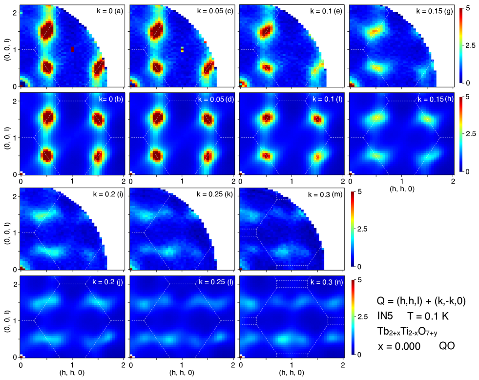
Figure 5: Intensity maps of 3D data $[S(\bm{Q})]_{\text{el}}$ taken at 0.1 K for the QO sample with $x=0.000$. The 3D data are viewed by 2D slices (a,c,e,g,i,k,m), which are parallel cross-sections of $\bm{Q}=(h,h,l)+(k,-k,0)$ with fixed $k$. These can be compared to the typical RPA $[S(\bm{Q})]_{\text{el}}$ (b,d,f,h,j,l,n) obtained by least squares fit using the 13 coupling constants, $J_{1},\cdots,J_{13}$, listed in Table 1. Dashed lines in these 2D slices (a-n) are boundaries of Brillouin zones.

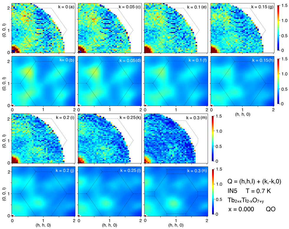
Figure 6: Intensity maps of 3D data $[S(\bm{Q})]_{\text{el}}$ taken at 0.7 K for the QO sample with $x=0.000$. The 3D data are viewed by 2D slices (a,c,e,g,i,k,m), which are parallel cross-sections of $\bm{Q}=(h,h,l)+(k,-k,0)$ with fixed $k$. These can be compared to the typical RPA $[S(\bm{Q})]_{\text{el}}$ (b,d,f,h,j,l,n) obtained by least squares fit using the 9 coupling constants, $J_{1},\cdots,J_{9}$, listed in Table 1. Dashed lines in these 2D slices (a-n) are boundaries of Brillouin zones.

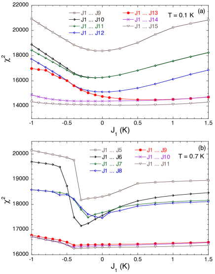
Figure 7: Minimized values of the weighted sum of squared residuals $\chi^{2}$ as a function of the fixed parameter $J_{1}$. (a) Results of least squares fits of $[S(\bm{Q})]_{\text{el}}$ with adjustable parameters $J_{m}$ ($m\leq m_{\text{max}}=9,\cdots,15$) for the QO sample with $x=0.000$ taken at $0.1$ K (Fig. 5). The number of fit data is 11418. (b) Results of least squares fits of $[S(\bm{Q})]_{\text{el}}$ with adjustable parameters $J_{m}$ ($m\leq m_{\text{max}}=5,\cdots,11$) for the QO sample with $x=0.000$ taken at 0.7 K (Fig. 6). The number of fit data is 10520.

We show 3D data sets $[S(\bm{Q})]_{\text{el}}$ for the QO sample with $x=0.000$ taken at 0.1 and 0.7 K in Fig. 5(a,c,e,g,i,k,m) and Fig. 6(a,c,e,g,i,k,m), respectively. By comparing these figures with the corresponding $[S(\bm{Q})]_{\text{el}}$ shown in Fig. 1 and Fig. 4 for the QSL sample, one can see that the 3D data $[S(\bm{Q})]_{\text{el}}$ of these QSL and QO samples show many similarities, which suggests a common origin. This is in stark contrast to the difference of their inelastic spectra shown in Fig. 2 of Ref. Kadowaki et al. (2018). Close inspection of the 3D data $[S(\bm{Q})]_{\text{el}}$ of Fig. 5 and Fig. 1 shows that the peaked structures at $\bm{Q}=(\tfrac{1}{2},\tfrac{1}{2},\tfrac{1}{2})$ and $(\tfrac{1}{2},\tfrac{1}{2},\tfrac{3}{2})$ of the QO sample are slightly broader than those of the QSL sample, and that the peak width of the QO sample is slightly larger than the QSL sample. This indicates that the small quadrupole order slightly suppresses the $\bm{q}=(\tfrac{1}{2},\tfrac{1}{2},\tfrac{1}{2})$ SRO.

We performed least squares fits of the observed 3D data sets $[S(\bm{Q})]_{\text{el}}$ to the RPA intensity Eq. (3), in the same way as those of the QSL sample. Resulting minimized values of $\chi^{2}$ are plotted as a function of the fixed $J_{1}$ in Fig. 7(a) and (b) for the 0.1 and 0.7 K data, respectively. These figures and Figs. 3(a) and (b) show that the least squares fits provided parallel results with those of the QSL sample. In fact, the typical coupling constants obtained by the fits, which are listed in Table 1, have many similarities for the two samples both at 0.1 and 0.7 K. Using these typical $J_{m}$ listed in Table 1 we calculated RPA $[S(\bm{Q})]_{\text{el}}$ and show them in Fig. 5(b,d,f,h,j,l,n) and Fig. 6(b,d,f,h,j,l,n). The observed and the calculated $[S(\bm{Q})]_{\text{el}}$ agree excellently and acceptably well at 0.1 K and 0.7 K, respectively.

III.3 QO sample with $x=0.003$

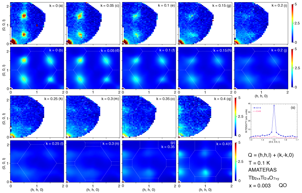
Figure 8: Intensity maps of 3D data $[S(\bm{Q})]_{\text{el}}$ taken at 0.1 K for the QO sample with $x=0.003$. The 3D data are viewed by 2D slices (a,c,e,g,i,k,m,o,q), which are parallel cross-sections of $\bm{Q}=(h,h,l)+(k,-k,0)$ with fixed $k$. These can be compared to the typical RPA $[S(\bm{Q})]_{\text{el}}$ (b,d,f,h,j,l,n,p,r) obtained by least squares fit using the 14 coupling constants, $J_{1},\cdots,J_{14}$, listed in Table 1. Dashed lines in these 2D slices (a-r) are boundaries of Brillouin zones. (s) $Q$-scan along $\bm{Q}=(\tfrac{1}{2},\tfrac{1}{2},l)$ close to magnetic reflection $(\tfrac{1}{2},\tfrac{1}{2},\tfrac{3}{2})$.

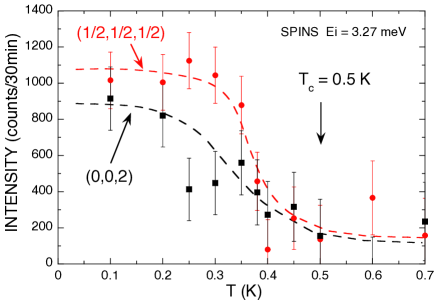
Figure 9: Temperature dependence of intensity of Bragg reflection of the powder sample with $x=0.005$ used in Ref. Taniguchi et al. (2013). These data were measured on the triple-axis spectrometer SPINS operated with $\lambda=5$ Å at NIST. Error bars represent one standard deviation.

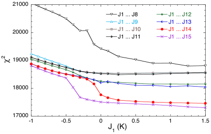
Figure 10: Minimized values of the weighted sum of squared residuals $\chi^{2}$ are plotted as a function of the fixed parameter $J_{1}$. These are obtained by least squares fits of $[S(\bm{Q})]_{\text{el}}$ with adjustable parameters $J_{m}$ ($m\leq m_{\text{max}}=8,\cdots,15$) for the QO sample with $x=0.003$ taken at $0.1$ K (Fig. 8). The number of fit data is 10570.

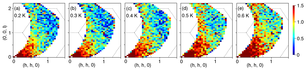
Figure 11: Temperature dependence of $[S(\bm{Q})]_{\text{el}}$ in the $(h,h,l)$ plane, where $k=0$ is fixed, for the QO sample with $x=0.003$. Dashed lines are boundaries of Brillouin zones.

Figure 8(a,c,e,g,i,k,m,o,q) shows a 3D data set $[S(\bm{Q})]_{\text{el}}$ taken at 0.1 K for the QO sample with $x=0.003$. These 3D data are substantially different from those of the QSL sample and the QO sample with $x=0.000$. The pinch point structure disappears. The $\bm{q}=(\tfrac{1}{2},\tfrac{1}{2},\tfrac{1}{2})$ SRO becomes much broader than that of the QO sample with $x=0.000$. Another new point of this sample is that there appears a tiny magnetic Bragg reflection at $\bm{Q}=(\tfrac{1}{2},\tfrac{1}{2},\tfrac{3}{2})$. A $Q$-scan through this reflection is plotted in Fig. 8(s), which shows that it disappears at 0.4 K. We note that detector gaps of AMATERAS prohibited us from measuring $\bm{Q}=(\tfrac{1}{2},\tfrac{1}{2},\tfrac{1}{2})$ and $(0,0,2)$ reflections.

The appearance of tiny magnetic Bragg reflections at $\bm{Q}=(\tfrac{1}{2},\tfrac{1}{2},\tfrac{3}{2})$, $(\tfrac{1}{2},\tfrac{1}{2},\tfrac{1}{2})$, and $(0,0,2)$ was reported only for samples with large quadrupole orders Taniguchi et al. (2013); Takatsu et al. (2016a); Guitteny et al. (2015). In order to complement our previous experimental data of the magnetic Bragg reflections shown in Fig. 5 of Ref. Taniguchi et al. (2013), we show temperature dependence of intensities of the Bragg reflections at $\bm{Q}=(\tfrac{1}{2},\tfrac{1}{2},\tfrac{1}{2})$ and $(0,0,2)$ in Fig. 9. Although statistical errors are large, one can see that the temperature dependence agrees with that shown in Fig. 3 of Ref. Takatsu et al. (2016a). Since several observations of the magnetic Bragg reflections have been accumulated, one may now have to accept the conclusion that the tiny magnetic Bragg reflections, indicating LRO of magnetic moments of the order $\sim 0.1\mu_{\text{B}}$, have a common origin attributed to the quadrupole LRO. They may possibly be caused by multi-spin interactions Mol ; Rau , which couple the magnetic and quadrupole moments.

We performed least squares fits of the 3D data set $[S(\bm{Q})]_{\text{el}}$ to the RPA intensity Eq. (3), in the same way as the QSL sample. In Fig. 10 we plot minimized values of $\chi^{2}$ as a function of the fixed $J_{1}$. This figure shows that as $J_{1}$ is decreased in the range $J_{1}<-5D/3$, the fits become unsatisfactory, and that the inclusion of further coupling constants $J_{m}$ with $m_{\text{max}}\geq 15$ does not improve the fitting. By inspecting several calculated $[S(\bm{Q})]_{\text{el}}$, we chose a typical good result of the fitting. This typical $[S(\bm{Q})]_{\text{el}}$ is shown in Fig. 8(b,d,f,h,j,l,n,p,r), which is calculated using the values of $J_{1},\cdots,J_{14}$ listed in Table 1. One can see that the agreement between the calculated and observed $[S(\bm{Q})]_{\text{el}}$ is not as good as that of the QSL sample. This less satisfactory agreement suggests that the quadrupole order breaks the space group symmetry. In fact, the proposed quadrupole order in Ref. Takatsu et al. (2016a) breaks this symmetry. We note that the typical coupling constants obtained by the fitting (Table 1) are substantially different from those of the QSL sample.

Figure 11 shows the temperature dependence of 2D intensity map in the plane $\bm{Q}=(h,h,l)$ observed in a temperature range $0.2\leq T\leq 0.6$ K. Although the $\bm{Q}$ range and statistical errors are limited, these 2D maps show that the $\bm{q}=(\tfrac{1}{2},\tfrac{1}{2},\tfrac{1}{2})$ SRO disappears already at 0.2 K. The pinch point structure around $(1,1,1)$, which is similar to that of the QSL sample at 0.7 K, is barely observable in the 0.3 and 0.4 K data. In the temperature range above 0.5 K, where the electric quadrupole order disappears, another kind of spin correlations seems to develop.

IV Discussion

A question of “what does $[S(\bm{Q})]_{\text{el}}$ measure?” is a little difficult to answer correctly. By the present definition, the (nominally) elastic scattering intensity $[S(\bm{Q})]_{\text{el}}=\int_{-\epsilon}^{\epsilon}S(\bm{Q},E)dE$ is defined on the basis of the present experimental conditions; thereby $[S(\bm{Q})]_{\text{el}}$ is different from theoretically elastic scattering. For the sake of simplicity as well as for our interest in the QLS state, we would like to discuss $[S(\bm{Q})]_{\text{el}}$ at the lowest temperature of the present experiments ($T=0.1$ K). Considering that this temperature scale is approximately equal to the instrumental energy resolution scales, $[S(\bm{Q})]_{\text{el}}$ at 0.1 K is essentially (and roughly) expressed by

$$\sum_{|E_{i}-E_{\text{G}}|,|E_{j}-E_{\text{G}}|<0.1\text{K}}\frac{e^{-\beta E_{i}}}{Z}|\langle j|\sum_{\bm{r}}\sigma_{\bm{r}}^{z}e^{i\bm{Q}\cdot\bm{r}}|i\rangle|^{2}\;,$$ (5)

where $E_{\text{G}}$ denotes the ground state energy and the summation runs over low-energy states, $|i\rangle$ and $|j\rangle$.

In the previous analyses of the $\bm{q}=(\tfrac{1}{2},\tfrac{1}{2},\tfrac{1}{2})$ SRO Fritsch et al. (2013); Guitteny et al. (2015), a few static Ising-spin clusters were assumed to exist, where certain disorders suppressing LRO are also assumed implicitly. These assumptions would be justified, if the system behaved within the classical spin paradigm, where the states $|i\rangle$ and $|j\rangle$ in Eq. (5) are expressed simply by single states described by the Ising-spin clusters. However, when quantum effects are included the simple low-energy states would be replaced by linear combinations of the Ising-spin-cluster states. As the number of Ising-spin-cluster states in a linear combination is increased, the system departs from the classical spin paradigm, and consequently the cluster analyses Fritsch et al. (2013); Guitteny et al. (2015) would not work properly. We speculate that the failures of obtaining sufficient goodness-of-fit in Refs. Fritsch et al. (2013); Guitteny et al. (2015) indicates that this really happened. For the present RPA analyses, although RPA takes account of quantum effects to a certain extent, RPA is basically a classical approach and thereby the same problem would occur, especially when quantum effects become substantially large, e.g., QSL states. We speculate that the breakdown of the classical paradigm is manifested as the necessity of the unexpectedly large number of coupling constants in the present RPA fitting.

The observed $[S(\bm{Q})]_{\text{el}}$ shown in Fig. 1 can be excellently reproduced by the RPA formulae Eq. (2) and Eq. (3). We think that there are two reasons for this successful fit. Firstly, the RPA formulae act as inverse Fourier transform. The many coupling constants imply that many inverse Fourier components are needed to reproduce the observed $[S(\bm{Q})]_{\text{el}}$. For example, the terms related to $J_{3}$ ($>0$) in Eq. (2) give rise to higher $[S(\bm{Q})]_{\text{el}}$ at wavevectors $\bm{Q}=(\tfrac{1}{2},\tfrac{1}{2},\tfrac{1}{2})$, $(\tfrac{1}{2},\tfrac{1}{2},\tfrac{3}{2})$ etc. Secondly, the coupling constants $J_{m}$ in Eq. (1) are allowed by the space group symmetry. As a consequence the RPA intensity formulae reflect the symmetry of the pyrochlore structure. In this sense, we may conclude that the QSL state of TTO retains the space group symmetry.

Apart from the analyses, one can obtain a few hints for further investigations of the QSL state of TTO directly from a few experimental facts. As discussed in section III.1, the 3D data set $[S(\bm{Q})]_{\text{el}}$ at 0.7 K (Fig. 4) shows the pinch point structure around $\bm{Q}=(1,1,1)$. This suggests that the QSI state proposed in Ref. Molavian et al. (2007) is somehow continuously connected to the QSL state of TTO. The tiny magnetic Bragg reflections observed in several QO samples, discussed in section III.3, are now regarded as an experimental fact. Thus the pseudospin-$\frac{1}{2}$ Hamiltonian is to be modified to include coupling between magnetic and quadrupole moments.

V Conclusions

Spin correlations of the frustrated pyrochlore oxide Tb_2+xTi_2-xO_7+y have been investigated by inelastic neutron scattering using single crystalline samples showing both the quantum-spin-liquid and quadrupole-ordered states. The observed spin correlations show pinch-point type structures around $\Gamma$ points, an antiferromagnetic short-range order around $L$ points, and tiny antiferromagnetic Bragg scattering at $L$ and $\Gamma$ points. The $\bm{q}=(\tfrac{1}{2},\tfrac{1}{2},\tfrac{1}{2})$ short-range order was analyzed using a model calculation of a random phase approximation assuming two-spin interactions among Ising spins. Analyses have shown that the RPA scattering intensity well reproduces the experimental data using temperature and $x$ dependent coupling constants of up to 10 neighbor site pairs. The unexpectedly large number of coupling constants required in the fitting suggest a breakdown of the classical spin paradigm at low temperatures and the necessity of a quantum spin paradigm.

Appendix A RPA model calculation and definitions

Methods of the RPA model calculation and related definitions are summarized in this section. The effective pseudospin-$\frac{1}{2}$ operators $\sigma_{\bm{r}}^{z}$ reside on the pyrochlore lattice sites $\bm{r}=\bm{t}_{n}+\bm{d}_{\nu}$, where $\bm{t}_{n}$ are FCC translation vectors and $\bm{d}_{\nu}$ are four crystallographic sites in the unit cell. These sites and their symmetry axes $\bm{x}_{\nu}$, $\bm{y}_{\nu}$, and $\bm{z}_{\nu}$ Kadowaki et al. (2015) are listed in Table 2. Representative site pairs $\langle{\bm{r}},{\bm{r}}^{\prime}\rangle_{m}$ of the coupling constants $J_{m}$ of Eq. (1) are listed in Table 3.

Table 2: Four crystallographic sites $\bm{d}_{\nu}$ ($\nu=0,1,2,3$) and their local symmetry axes $\bm{x}_{\nu}$, $\bm{y}_{\nu}$, and $\bm{z}_{\nu}$ Kadowaki et al. (2015).

$\nu$	$\bm{d}_{\nu}$	$\bm{x}_{\nu}$	$\bm{y}_{\nu}$	$\bm{z}_{\nu}$
0	$\tfrac{1}{4}(0,0,0)$	$\tfrac{1}{\sqrt{6}}(1,1,-2)$	$\tfrac{1}{\sqrt{2}}(-1,1,0)$	$\tfrac{1}{\sqrt{3}}(1,1,1)$
1	$\tfrac{1}{4}(0,1,1)$	$\tfrac{1}{\sqrt{6}}(1,-1,2)$	$\tfrac{1}{\sqrt{2}}(-1,-1,0)$	$\tfrac{1}{\sqrt{3}}(1,-1,-1)$
2	$\tfrac{1}{4}(1,0,1)$	$\tfrac{1}{\sqrt{6}}(-1,1,2)$	$\tfrac{1}{\sqrt{2}}(1,1,0)$	$\tfrac{1}{\sqrt{3}}(-1,1,-1)$
3	$\tfrac{1}{4}(1,1,0)$	$\tfrac{1}{\sqrt{6}}(-1,-1,-2)$	$\tfrac{1}{\sqrt{2}}(1,-1,0)$	$\tfrac{1}{\sqrt{3}}(-1,-1,1)$

Table 3: Representative site pairs $\langle{\bm{r}},{\bm{r}}^{\prime}\rangle_{m}=\langle\bm{t}_{n}+\bm{d}_{\nu},\bm{t}_{n^{\prime}}+\bm{d}_{\nu^{\prime}}\rangle_{m}$ of the coupling constants $J_{m}$ of Eq. (1) are listed using $(\nu,\nu^{\prime})$ and ${\bm{r}}^{\prime}-{\bm{r}}$. Distances between the site pairs $|{\bm{r}}^{\prime}-{\bm{r}}|$ show that the constants $J_{m}$ in this list are up to 11 neighbor coupling, and that for 3, 7, 9, and 10 neighbor site pairs, there are 2, 2, 3, and 2 non-equivalent site pairs, respectively.

$J_{m}$	$(\nu,\nu^{\prime})$	${\bm{r}}^{\prime}-{\bm{r}}$	$|{\bm{r}}^{\prime}-{\bm{r}}|$
$J_{1}$	(0,1)	(0 , 1/4 , 1/4)	0.35355
$J_{2}$	(0,1)	(1/2 , 1/4 , -1/4)	0.61237
$J_{3}$	(0,0)	(1/2 , 1/2 , 0 )	0.70710
$J_{4}$	(0,0)	(1/2 , -1/2 , 0 )	0.70710
$J_{5}$	(0,1)	(0 , 3/4 , -1/4)	0.79057
$J_{6}$	(0,1)	(1/2 , 1/4 , 3/4)	0.93541
$J_{7}$	(0,0)	(1 , 0 , 0 )	1
$J_{8}$	(0,1)	(1 , 1/4 , 1/4)	1.06066
$J_{9}$	(0,1)	(0 , 3/4 , 3/4)	1.06066
$J_{10}$	(0,1)	(1/2 , 3/4 , -3/4)	1.17260
$J_{11}$	(0,0)	(1 , -1/2 , -1/2)	1.224745
$J_{12}$	(0,0)	(1 , 1/2 , -1/2)	1.224745
$J_{13}$	(0,0)	(1 , 1/2 , 1/2)	1.224745
$J_{14}$	(0,1)	(0 , 5/4 , 1/4)	1.274755
$J_{15}$	(0,1)	(1 , 3/4 , -1/4)	1.274755
$J_{16}$	(0,1)	(1/2 , 5/4 , -1/4)	1.36930

The generalized susceptibility $\chi_{\nu^{\prime\prime},\nu^{\prime}}(\bm{k},E)$, where $\bm{k}$ is a vector in the FCC first Brillouin zone, is computed by solving an RPA equation Jensen and Mackintosh (1991)

$$\sum_{\nu^{\prime\prime}}[\delta_{\nu,\nu^{\prime\prime}}-\sum_{\nu^{\prime\prime\prime}}\chi^{0}_{\nu,\nu^{\prime\prime\prime}}(E)J_{\nu^{\prime\prime\prime},\nu^{\prime\prime}}(\bm{k})]\chi_{\nu^{\prime\prime},\nu^{\prime}}(\bm{k},E)=\chi^{0}_{\nu,\nu^{\prime}}(E)\;,$$ (6)

where $J_{\nu,\nu^{\prime}}(\bm{k})$ denotes the Fourier transform of the magnetic coupling constants $J_{n,\nu;n^{\prime},\nu^{\prime}}$ between sites $\bm{t}_{n^{\prime}}+\bm{d}_{\nu^{\prime}}$ and $\bm{t}_{n}+\bm{d}_{\nu}$

$$J_{\nu,\nu^{\prime}}(\bm{k})=\sum_{n}J_{n,\nu;n^{\prime},\nu^{\prime}}e^{i\bm{k}\cdot[(\bm{t}_{n}+\bm{d}_{\nu})-(\bm{t}_{n^{\prime}}+\bm{d}_{\nu^{\prime}})]}\;,$$ (7)

and $\chi^{0}_{\nu,\nu^{\prime}}(E)$ is the single site susceptibility. In the paramagnetic phase

$$\chi^{0}_{\nu,\nu^{\prime}}(E)=\delta_{\nu,\nu^{\prime}}\chi_{\text{L}}\frac{\Gamma_{0}}{\Gamma_{0}-iE}\;,$$ (8)

where $\chi_{\text{L}}=1/(4k_{\text{B}}T)$ is the local susceptibility Jensen and Mackintosh (1991) and $\Gamma_{0}$ is a small positive constant.

The neutron magnetic scattering intensity $S(\bm{Q}=\bm{G}+\bm{k},E)$, where $\bm{G}$ is a reciprocal lattice vector, is given by

$$S(\bm{Q},E)\propto f(Q)^{2}\frac{1}{1-e^{-\beta E}}\sum_{\rho,\sigma,\nu,\nu^{\prime}}(\delta_{\rho,\sigma}-\hat{Q}_{\rho}\hat{Q}_{\sigma})$$

$$\times U_{\rho,z}^{(\nu)}U_{\sigma,z}^{(\nu^{\prime})}\text{Im}\left\{\chi_{\nu,\nu^{\prime}}(\bm{k},E)e^{-i\bm{G}\cdot(\bm{d}_{\nu}-\bm{d}_{\nu^{\prime}})}\right\}\;,$$ (9)

where $U_{\rho,\alpha}^{(\nu)}$ is the rotation matrix from the local ($\alpha$) frame defined at the sites $\bm{t}_{n}+\bm{d}_{\nu}$ to the global ($\rho$) frame Kao et al. (2003); Kadowaki et al. (2015). In the quasi-elastic approximation, the elastic scattering intensity $[S(\bm{Q})]_{\text{el}}$ is given by integrating Eq. (9) in a small range $|E|<\epsilon$

$$[S(\bm{Q})]_{\text{el}}=\int_{-\epsilon}^{\epsilon}S(\bm{Q},E)dE\propto f(Q)^{2}\sum_{\rho,\sigma,\nu,\nu^{\prime}}(\delta_{\rho,\sigma}-\hat{Q}_{\rho}\hat{Q}_{\sigma})$$

$$\times U_{\rho,z}^{(\nu)}U_{\sigma,z}^{(\nu^{\prime})}\int_{-\epsilon}^{\epsilon}\frac{\text{Im}\left\{\chi_{\nu,\nu^{\prime}}(\bm{k},E)e^{-i\bm{G}\cdot(\bm{d}_{\nu}-\bm{d}_{\nu^{\prime}})}\right\}}{E}dE$$

$$\propto f(Q)^{2}\sum_{\rho,\sigma,\nu,\nu^{\prime}}(\delta_{\rho,\sigma}-\hat{Q}_{\rho}\hat{Q}_{\sigma})U_{\rho,z}^{(\nu)}U_{\sigma,z}^{(\nu^{\prime})}$$

$$\;\;\;\;\;\;\;\;\;\;\;\;\times\chi_{\nu,\nu^{\prime}}(\bm{k},0)\cos[\bm{G}\cdot(\bm{d}_{\nu}-\bm{d}_{\nu^{\prime}})]\;,$$ (10)

where $\Gamma_{0}\ll\epsilon$ is assumed.

Appendix B Least squares fit

Technical details of the least squares fits are summarized in this section. The computations of the least squares fits were performed on the CX400 supercomputer NIS using a non-linear least squares program Kadowaki (b) based on the Levenberg-Marquardt algorithm. The difficulty of the present minimization problem of $\chi^{2}$ [Eq. (4)] is caused by a fact that $\chi^{2}$ has many local minima in the parameter space. A trivial origin of this difficulty is that infinitesimal changes of $J_{\text{nn,eff}}\rightarrow(1+\epsilon)J_{\text{nn,eff}}$, where $J_{\text{nn,eff}}=J_{1}+\tfrac{3}{5}D$ ($>0$) is the effective ferromagnetic NN coupling for small $J_{m}$ ($m\geq 2$) den Hertog and Gingras (2000), $J_{m}\rightarrow(1+\epsilon)J_{m}$ ($m\geq 2$), and $\chi_{\text{L}}\rightarrow(1-\epsilon)\chi_{\text{L}}$ in Eq. (6) bring about $[S(\bm{Q})]_{\text{el}}\rightarrow(1-\epsilon)[S(\bm{Q})]_{\text{el}}$ [Eq. (10)], and consequently do not change the $\bm{Q}$ dependence of $[S(\bm{Q})]_{\text{el}}$. To avoid the (nearly) rank deficiency in the QR decomposition due to this fact, we fixed $J_{1}$ in performing the least squares fits. Indications of occurrence of this problem can be seen as several ranges of $\chi^{2}\simeq\text{const.}$ in the curves of Figs. 3, 7, and 10. In addition, there were other unknown origins for the many local minima. These difficulties could be avoided by introducing a weak constraint of the parameters, i.e., adding the penalty function $\sum_{2\leq m\leq m_{\text{max}}}\left(\tfrac{J_{m}}{1\text{ K}}\right)^{8}$ to $\chi^{2}$. This penalty function weakly restricts $J_{m}$ in the range $|J_{m}|<1$ K, which is a reasonable assumption, and can be treated in the framework of the Levenberg-Marquardt algorithm. By inspecting results of the least squares fits, we can conclude that sufficiently accurate solutions of the minimization problem were obtained for the present purpose Sup . The uncertainty of the typical coupling constants listed in Table 1 is of the order 0.1 K Sup .

References

- Wannier (1950) G. H. Wannier, Phys. Rev. 79, 357 (1950).
- Syôzi (1951) I. Syôzi, Prog. Theor. Phys. 6, 306 (1951).
- Qi et al. (2008) Y. Qi, T. Brintlinger, and J. Cumings, Phys. Rev. B 77, 094418 (2008).
- Gardner et al. (2010) J. S. Gardner, M. J. P. Gingras, and J. E. Greedan, Rev. Mod. Phys. 82, 53 (2010).
- Lacroix et al. (2011) C. Lacroix, P. Mendels, and F. Mila, eds., Introduction to Frustrated Magnetism (Springer, Berlin, Heidelberg, 2011).
- Bramwell and Gingras (2001) S. T. Bramwell and M. J. P. Gingras, Science 294, 1495 (2001).
- Ramirez et al. (1999) A. P. Ramirez, A. Hayashi, R. J. Cava, R. Siddharthan, and B. S. Shastry, Nature (London) 399, 333 (1999).
- Matsuhira et al. (2002) K. Matsuhira, Z. Hiroi, T. Tayama, S. Takagi, and T. Sakakibara, J. Phys. Condens. Matter 14, L559 (2002).
- Castelnovo et al. (2008) C. Castelnovo, R. Moessner, and S. L. Sondhi, Nature 451, 42 (2008).
- Kadowaki et al. (2009) H. Kadowaki, N. Doi, Y. Aoki, Y. Tabata, T. J. Sato, J. W. Lynn, K. Matsuhira, and Z. Hiroi, J. Phys. Soc. Jpn. 78, 103706 (2009).
- Kadowaki and Nishimori (1998) T. Kadowaki and H. Nishimori, Phys. Rev. E 58, 5355 (1998).
- King et al. (2018) A. D. King, J. Carrasquilla, I. Ozfidan, J. Raymond, E. Andriyash, A. Berkley, M. Reis, T. M. Lanting, R. Harris, G. Poulin-Lamarre, A. Y. Smirnov, C. Rich, F. Altomare, P. Bunyk, J. Whittaker, L. Swenson, E. Hoskinson, Y. Sato, M. Volkmann, E. Ladizinsky, M. Johnson, J. Hilton, and M. H. Amin, Nature (London) 560, 456 (2018).
- Savary and Balents (2017) L. Savary and L. Balents, Rep. Prog. Phys. 80, 016502 (2017).
- Anderson (1973) P. W. Anderson, Mater. Res. Bull. 8, 153 (1973).
- Hirakawa et al. (1985) K. Hirakawa, H. Kadowaki, and K. Ubukoshi, J. Phys. Soc. Jpn. 54, 3526 (1985).
- Gardner et al. (1999) J. S. Gardner, S. R. Dunsiger, B. D. Gaulin, M. J. P. Gingras, J. E. Greedan, R. F. Kiefl, M. D. Lumsden, W. A. MacFarlane, N. P. Raju, J. E. Sonier, I. Swainson, and Z. Tun, Phys. Rev. Lett. 82, 1012 (1999).
- Han et al. (2012) T.-H. Han, J. S. Helton, S. Chu, D. G. Nocera, J. A. Rodriguez-Rivera, C. Broholm, and Y. S. Lee, Nature (London) 492, 406 (2012).
- Ross et al. (2011) K. A. Ross, L. Savary, B. D. Gaulin, and L. Balents, Phys. Rev. X 1, 021002 (2011).
- Chang et al. (2012) L.-J. Chang, S. Onoda, Y. Su, Y.-J. Kao, K.-D. Tsuei, Y. Yasui, K. Kakurai, and M. R. Lees, Nature Communications 3, 992 (2012).
- Shen et al. (2016) Y. Shen, Y.-D. Li, H. Wo, Y. Li, S. Shen, B. Pan, Q. Wang, H. C. Walker, P. Steffens, M. Boehm, Y. Hao, D. L. Quintero-Castro, L. W. Harriger, M. D. Frontzek, L. Hao, S. Meng, Q. Zhang, G. Chen, and J. Zhao, Nature (London) 540, 559 (2016).
- Fåk et al. (2017) B. Fåk, S. Bieri, E. Canévet, L. Messio, C. Payen, M. Viaud, C. Guillot-Deudon, C. Darie, J. Ollivier, and P. Mendels, Phys. Rev. B 95, 060402 (2017).
- Sibille et al. (2018) R. Sibille, N. Gauthier, H. Yan, M. Ciomaga Hatnean, J. Ollivier, B. Winn, U. Filges, G. Balakrishnan, M. Kenzelmann, N. Shannon, and T. Fennell, Nature Physics 14, 711 (2018).
- Kadowaki et al. (2018) H. Kadowaki, M. Wakita, B. Fåk, J. Ollivier, S. Ohira-Kawamura, K. Nakajima, H. Takatsu, and M. Tamai, J. Phys. Soc. Jpn. 87, 064704 (2018).
- Molavian et al. (2007) H. R. Molavian, M. J. P. Gingras, and B. Canals, Phys. Rev. Lett. 98, 157204 (2007).
- Gingras and McClarty (2014) M. J. P. Gingras and P. A. McClarty, Rep. Prog. Phys. 77, 056501 (2014).
- Taniguchi et al. (2013) T. Taniguchi, H. Kadowaki, H. Takatsu, B. Fåk, J. Ollivier, T. Yamazaki, T. J. Sato, H. Yoshizawa, Y. Shimura, T. Sakakibara, T. Hong, K. Goto, L. R. Yaraskavitch, and J. B. Kycia, Phys. Rev. B 87, 060408 (2013).
- Wakita et al. (2016) M. Wakita, T. Taniguchi, H. Edamoto, H. Takatsu, and H. Kadowaki, J. Phys.: Conf. Series 683, 012023 (2016).
- Takatsu et al. (2016a) H. Takatsu, S. Onoda, S. Kittaka, A. Kasahara, Y. Kono, T. Sakakibara, Y. Kato, B. Fåk, J. Ollivier, J. W. Lynn, T. Taniguchi, M. Wakita, and H. Kadowaki, Phys. Rev. Lett. 116, 217201 (2016a).
- Takatsu et al. (2016b) H. Takatsu, T. Taniguchi, S. Kittaka, T. Sakakibara, and H. Kadowaki, J. Phys.: Conf. Series 683, 012022 (2016b).
- Kadowaki et al. (2018) H. Kadowaki, H. Takatsu, and M. Wakita, Phys. Rev. B 98, 144410 (2018).
- Onoda and Tanaka (2011) S. Onoda and Y. Tanaka, Phys. Rev. B 83, 094411 (2011).
- Lee et al. (2012) S. Lee, S. Onoda, and L. Balents, Phys. Rev. B 86, 104412 (2012).
- Hermele et al. (2004) M. Hermele, M. P. A. Fisher, and L. Balents, Phys. Rev. B 69, 064404 (2004).
- Yasui et al. (2002) Y. Yasui, M. Kanada, M. Ito, H. Harashina, M. Sato, H. Okumura, K. Kakurai, and H. Kadowaki, J. Phys. Soc. Jpn. 71, 599 (2002).
- Fennell et al. (2012) T. Fennell, M. Kenzelmann, B. Roessli, M. K. Haas, and R. J. Cava, Phys. Rev. Lett. 109, 017201 (2012).
- Petit et al. (2012) S. Petit, P. Bonville, J. Robert, C. Decorse, and I. Mirebeau, Phys. Rev. B 86, 174403 (2012).
- Fritsch et al. (2013) K. Fritsch, K. A. Ross, Y. Qiu, J. R. D. Copley, T. Guidi, R. I. Bewley, H. A. Dabkowska, and B. D. Gaulin, Phys. Rev. B 87, 094410 (2013).
- Guitteny et al. (2015) S. Guitteny, I. Mirebeau, P. Dalmas de Réotier, C. V. Colin, P. Bonville, F. Porcher, B. Grenier, C. Decorse, and S. Petit, Phys. Rev. B 92, 144412 (2015).
- Jensen and Mackintosh (1991) J. Jensen and A. R. Mackintosh, Rare Earth Magnetism (Clarendon Press, Oxford, 1991).
- Kadowaki et al. (2015) H. Kadowaki, H. Takatsu, T. Taniguchi, B. Fåk, and J. Ollivier, SPIN 05, 1540003 (2015).
- Takatsu et al. (2017) H. Takatsu, T. Taniguchi, S. Kittaka, T. Sakakibara, and H. Kadowaki, J. Phys.: Conf. Series 828, 012007 (2017).
- Fak (a) B. Fåk, H. Kadowaki, J. Ollivier and M. Wakita. (2015). Quadrupole order of Tb2+xTi2-xO7+y. Institut Laue-Langevin (ILL) doi:10.5291/ILL-DATA.4-05-628.
- Fak (b) B. Fåk, H. Kadowaki, and J. Ollivier. (2016). Quadrupole order of Tb2+xTi2-xO7+y. Institut Laue-Langevin (ILL) doi:10.5291/ILL-DATA.4-05-635.
- Kadowaki (a) H. Kadowaki, https://github.com/kadowaki-h/AbsorptionFactorIN5; https://github.com/kadowaki-h/AbsorptionFactorAMATERAS.
- Ewings et al. (2016) R. Ewings, A. Buts, M. Le, J. van Duijn, I. Bustinduy, and T. Perring, Nucl. Instrum. Methods Phys. Res. Sect. A 834, 132 (2016).
- den Hertog and Gingras (2000) B. C. den Hertog and M. J. P. Gingras, Phys. Rev. Lett. 84, 3430 (2000).
- (47) See Supplemental Material at https for further details of the least squares fits.
- Li et al. (2013) Q. J. Li, Z. Y. Zhao, C. Fan, F. B. Zhang, H. D. Zhou, X. Zhao, and X. F. Sun, Phys. Rev. B 87, 214408 (2013).
- Kermarrec et al. (2015) E. Kermarrec, D. D. Maharaj, J. Gaudet, K. Fritsch, D. Pomaranski, J. B. Kycia, Y. Qiu, J. R. D. Copley, M. M. P. Couchman, A. O. R. Morningstar, H. A. Dabkowska, and B. D. Gaulin, Phys. Rev. B 92, 245114 (2015).
- Fennell et al. (2009) T. Fennell, P. P. Deen, A. R. Wildes, K. Schmalzl, D. Prabhakaran, A. T. Boothroyd, R. J. Aldus, D. F. McMorrow, and S. T. Bramwell, Science 326, 415 (2009).
- (51) H. R. Molavian, P. A. McClarty, and M. J. P. Gingras, arXiv:0912.2957.
- (52) J. G. Rau and M. J. P. Gingras, arXiv:1806.09638.
- (53) The identification of any commercial product or trade name does not imply endorsement or recommendation by the National Institute of Standards and Technology.
- Kao et al. (2003) Y.-J. Kao, M. Enjalran, A. Del Maestro, H. R. Molavian, and M. J. P. Gingras, Phys. Rev. B 68, 172407 (2003).
- Kadowaki (b) H. Kadowaki, https://github.com/kadowaki-h/least65OMP.