22email: {yangze,luotg,wangdongcis,huzq,jun.gao}@pku.edu.cn
wanglw@cis.pku.edu.cn
Learning to Navigate for Fine-grained Classification
Abstract
Fine-grained classification is challenging due to the difficulty of finding discriminative features. Finding those subtle traits that fully characterize the object is not straightforward. To handle this circumstance, we propose a novel self-supervision mechanism to effectively localize informative regions without the need of bounding-box/part annotations. Our model, termed NTS-Net for Navigator-Teacher-Scrutinizer Network, consists of a Navigator agent, a Teacher agent and a Scrutinizer agent. In consideration of intrinsic consistency between informativeness of the regions and their probability being ground-truth class, we design a novel training paradigm, which enables Navigator to detect most informative regions under the guidance from Teacher. After that, the Scrutinizer scrutinizes the proposed regions from Navigator and makes predictions. Our model can be viewed as a multi-agent cooperation, wherein agents benefit from each other, and make progress together. NTS-Net can be trained end-to-end, while provides accurate fine-grained classification predictions as well as highly informative regions during inference. We achieve state-of-the-art performance in extensive benchmark datasets.
1 Introduction
Fine-grained classification aims at differentiating subordinate classes of a common superior class, e.g. distinguishing wild bird species, automobile models, etc. Those subordinate classes are usually defined by domain experts with complicated rules, which typically focus on subtle differences in particular regions. While deep learning has promoted the research in many computer vision [24, 38, 33] tasks, its application in fine-grained classification is more or less unsatisfactory, due in large part to the difficulty of finding informative regions and extracting discriminative features therein. The situation is even worse for subordinate classes with varied poses like birds.
As a result, the key to fine-grained classification lies in developing automatic methods to accurately identify informative regions in an image. Some previous works [45, 8, 3, 46, 13, 2, 29] take advantage of fine-grained human annotations, like annotations for bird parts in bird classification. While achieving decent results, the fine-grained human annotations they require are expensive, making those methods less applicable in practice. Other methods [49, 47, 48, 43] employ an unsupervised learning scheme to localize informative regions. They eliminate the need for the expensive annotations, but lack a mechanism to guarantee that the model focuses on the right regions, which usually results in degraded accuracy.
In this paper, we propose a novel self-supervised mechanism to effectively localize informative regions without the need of fine-grained bounding-box/part annotations. The model we develop, which we term NTS-Net for Navigator-Teacher-Scrutinizer Network, employs a multi-agent cooperative learning scheme to address the problem of accurately identifying informative regions in an image. Intuitively, the regions assigned higher probability to be ground-truth class should contain more object-characteristic semantics enhancing the classification performance of the whole image. Thus we design a novel loss function to optimize the informativeness of each selected region to have the same order as its probability being ground-truth class, and we take the ground-truth class of full image as the ground-truth class of regions.
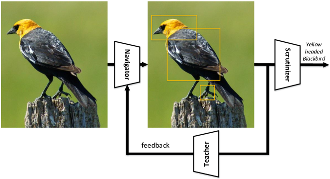
Specifically, our NTS-Net consists of a Navigator agent, a Teacher agent and a Scrutinizer agent. The Navigator navigates the model to focus on the most informative regions: for each region in the image, Navigator predicts how informative the region is, and the predictions are used to propose the most informative regions. The Teacher evaluates the regions proposed by Navigator and provides feedbacks: for each proposed region, the Teacher evaluates its probability belonging to ground-truth class; the confidence evaluations guide the Navigator to propose more informative regions with our novel ordering-consistent loss function. The Scrutinizer scrutinizes proposed regions from Navigator and makes fine-grained classifications: each proposed region is enlarged to the same size and the Scrutinizer extracts features therein; the features of regions and of the whole image are jointly processed to make fine-grained classifications. As a whole, our method can be viewed as an actor-critic [21] scheme in reinforcement learning, where the Navigator is the actor and the Teacher is the critic. With a more precise supervision provided by the Teacher, the Navigator will localize more informative regions, which in turn will benefit the Teacher. As a result, agents make progress together and end up with a model which provides accurate fine-grained classification predictions as well as highly informative regions. Fig. 1 shows an overview of our methods.
Our main contributions can be summarized as follows:
-
•
We propose a novel multi-agent cooperative learning scheme to address the problem of accurately identifying informative regions in the fine-grained classification task without bounding-box/part annotations.
-
•
We design a novel loss function, which enables Teacher to guide Navigator to localize the most informative regions in an image by enforcing the consistency between regions’ informativeness and their probability being ground-truth class.
-
•
Our model can be trained end-to-end, while provides accurate fine-grained classification predictions as well as highly informative regions during inference. We achieve state-of-the-art performance in extensive benchmark datasets.
2 Related Work
2.1 Fine-grained classification
There have been a variety of methods designed to distinguish fine-grained categories. Since some fine-grained classification datasets provide bounding-box/part annotations, early works [45, 8, 2] take advantage of those annotations at both training and inference phase. However in practice when the model is deployed, no human annotations will be available. Later on, some works [3, 46] use bounding-box/part annotations only at training phase. Under this setting, the framework is quite similar to detection: selecting regions and then classifying the pose-normalized objects. Besides, Jonathan et al. [22] use co-segmentation and alignment to generate parts without part annotations but the bounding-box annotations are used during training. Recently, a more general setting has emerged that does not require bounding box/part annotations either at training or inference time. This setting makes fine-grained classification more useful in practice. This paper will mainly consider the last setting, where bounding-box/part annotations are not needed either at training or inference phase.
In order to learn without fine-grained annotations, Jaderberg et al. [19] propose Spatial Transformer Network to explicitly manipulate data representation within the network and predict the location of informative regions. Lin et al. [28] use a bilinear model to build discriminative features of the whole image; the model is able to capture subtle differences between different subordinate classes. Zhang et al. [47] propose a two-step approach to learn a bunch of part detectors and part saliency maps. Fu et al. [12] use an alternate optimization scheme to train attention proposal network and region-based classifier; they show that two tasks are correlated and can benefit each other. Zhao et al. [48] propose Diversified Visual Attention Network (DVAN) to explicitly pursues the diversity of attention and better gather discriminative information. Lam et al. [25] propose a Heuristic-Successor Network (HSNet) to formulate the fine-grained classification problem as a sequential search for informative regions in an image.
2.2 Object detection
Early object detection methods employ SIFT [34] or HOG [10] features. Recent works are mainly focusing on convolutional neural networks. Approaches like R-CNN [14], OverFeat [40] and SPPnet [16] adopt traditional image-processing methods to generate object proposals and perform category classification and bounding box regression. Later works like Faster R-CNN [38] propose Region Proposal Network (RPN) for proposal generation. YOLO [37] and SSD [31] improve detection speed over Faster R-CNN [38] by employing a single-shot architecture. On the other hand, Feature Pyramid Networks (FPN) [27] focuses on better addressing multi-scale problem and generates anchors from multiple feature maps. Our method requires selecting informative regions, which can also be viewed as object detection. To the best of our knowledge, we are the first one to introduce FPN into fine-grained classification while eliminates the need of human annotations.
2.3 Learning to rank
Learning to rank is drawing attention in the field of machine learning and information retrieval [30]. The training data consist of lists of items with assigned orders, while the objective is to learn the order for item lists. The ranking loss function is designed to penalize pairs with wrong order. Let denote the objects to rank, and the indexing of the objects, where means should be ranked before . Let be the hypothesis set of ranking function. The goal is to find a ranking function that minimize a certain loss function defined on , and . There are many ranking methods. Generally speaking, these methods can be divided into three categories: the point-wise approach [9], pair-wise approach [18, 4] and list-wise approach[6, 44].
Point-wise approach assign each data with a numerical score, and the learning-to-rank problem can be formulated as a regression problem, for example with loss function:
| (1) |
In the pair-wise ranking approach, the learning-to-rank problem is formulated as a classification problem. i.e. to learn a binary classifier that chooses the superiority in a pair. Suppose only takes a value from , where means is ranked before . Then the loss is defined on all pairs as in Eqn. 2, and the goal is to find an optimal to minimize the average number of pairs with wrong order.
| (2) |
List-wise approach directly optimizes the whole list, and it can be formalized as a classification problem on permutations. Let be the ranking function, the loss is defined as:
| (3) |
In our approach, our navigator loss function adopts from the multi-rating pair-wise ranking loss, which enforces the consistency between region’s informativeness and probability being ground-truth class.
3 Methods
3.1 Approach Overview
Our approach rests on the assumption that informative regions are helpful to better characterize the object, so fusing features from informative regions and the full image will achieve better performance. Therefore the goal is to localize the most informative regions of the objects. We assume all regions111Without loss of generality, we also treat full image as a region are rectangle, and we denote as the set of all regions in the given image222Notation: we use alligraphy font to denote mapping, lackboard bold font to denote special sets, And we use old font to denote parameters in network.. We define information function evaluating how informative the region is, and we define the confidence function as a classifier to evaluate the confidence that the region belongs to ground-truth class. As mentioned in Sec. 1, more informative regions should have higher confidence, so the following condition should hold:
-
Condition. 1: for any , if ,
We use Navigator network to approximate information function and Teacher network to approximate confidence function . For the sake of simplicity, we choose regions in the region space . For each region , the Navigator network evaluates its informativeness , and the Teacher network evaluates its confidence . In order to satisfy Condition. 1, we optimize Navigator network to make and having the same order.
As the Navigator network improves in accordance with the Teacher network, it will produce more informative regions to help Scrutinizer network make better fine-grained classification result.
In Section. 3.2, we will describe how informative regions are proposed by Navigator under Teacher’s supervision. In Section. 3.3, we will present how to get fine-grained classification result from Scrutinizer. In Section. 3.4 and 3.5, we will introduce the network architecture and optimization in detail, respectively.
3.2 Navigator and Teacher
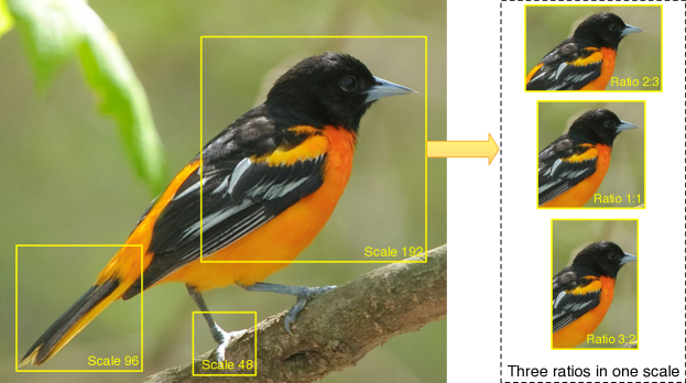
Navigating to possible informative regions can be viewed as a region proposal problem, which has been widely studied in [41, 11, 1, 7, 20]. Most of them are based on a sliding-windows search mechanism. Ren et al. [38] introduce a novel region proposal network (RPN) that shares convolutional layers with the classifier and mitigates the marginal cost for computing proposals. They use anchors to simultaneously predict multiple region proposals. Each anchor is associated with a sliding window position, aspect ratio, and box scale. Inspired by the idea of anchors, our Navigator network takes an image as input, and produce a bunch of rectangle regions , each with a score denoting the informativeness of the region (Fig. 2 shows the design of our anchors). For an input image of size 448, we choose anchors to have scales of {48, 96, 192} and ratios {1:1, 3:2, 2:3}, then Navigator network will produce a list denoting the informativeness of all anchors. We sort the information list as in Eqn. 4 , where is the number of anchors, is the -th element in sorted information list.
| (4) |
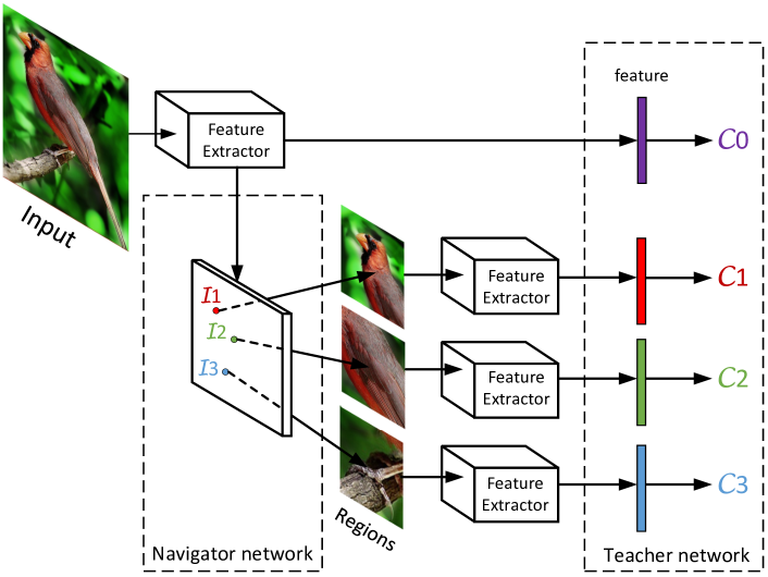
To reduce region redundancy, we adopt non-maximum suppression (NMS) on the regions based on their informativeness. Then we take the top- informative regions and feed them into the Teacher network to get the confidence as . Fig. 3 shows the overview with , where is a hyper-parameters denoting how many regions are used to train Navigator network. We optimize Navigator network to make and having the same order. Every proposed region is used to optimize Teacher by minimizing the cross-entropy loss between ground-truth class and the predicted confidence.
3.3 Scrutinizer
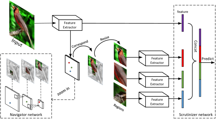
As Navigator network gradually converges, it will produce informative object-characteristic regions to help Scrutinizer network make decisions. We use the top- informative regions combined with the full image as input to train the Scrutinizer network. In other words, those regions are used to facilitate fine-grained recognition. Fig. 4 demonstrates this process with . Lam et al. [25] show that using informative regions can reduce intra-class variance and are likely to generate higher confidence scores on the correct label. Our comparative experiments show that adding informative regions substantially improve fine-grained classification results in a wide range of datasets including CUB-200-2001, FGVC Aircraft, and Stanford Cars, which are shown in Table. 2, 3.
3.4 Network architecture
In order to obtain correspondence between region proposals and feature vectors in feature map, we use fully-convolutional network as the feature extractor, without fully-connected layers. Specifically, we choose ResNet-50 [17] pre-trained on ILSVRC2012 [39] as the CNN feature extractor, and Navigator, Scrutinizer, Teacher network all share parameters in feature extractor. We denote parameters in feature extractor as . For input image , the extracted deep representations are denoted as , where denotes the combinations of convolution, pooling, and activation operations.
Navigator network.
Inspired by the design of Feature Pyramid Networks (FPN) [27], we use a top-down architecture with lateral connections to detect multi-scale regions. We use convolutional layers to compute feature hierarchy layer by layer, followed by ReLU activation and max-pooling. Then we get a series of feature maps of different spatial resolutions. The anchors in larger feature maps correspond to smaller regions. Navigator network in Figure. 4 shows the sketch of our design. Using multi-scale feature maps from different layers we can generate informativeness of regions among different scales and ratios. In our setting, we use feature maps of size corresponding to regions of scale . We denote the parameters in Navigator network as (including shared parameters in feature extractor).
Teacher network.
The Teacher network (Fig. 3) approximates the mapping which denotes the confidence of each region. After receiving scale-normalized () informative regions from Navigator network, Teacher network outputs confidence as teaching signals to help Navigator network learn. In addition to the shared layers in feature extractor, the Teaching network has a fully connected layer which has neurons. We denote the parameters in Teacher network as for convenience.
Scrutinizer network.
After receiving top- informative regions from Navigator network, the regions are resized to the pre-defined size (in our experiments we use ) and are fed into feature extractor to generate those regions’ feature vector, each with length . Then we concatenate those features with input image’s feature, and feed it into a fully-connected layer which has neurons (Fig. 4). We use function to represent the composition of these transformations. We denote the parameters in Scrutinizer network as .
3.5 Loss function and Optimization
Navigation loss. We denote the most informative regions predicted by Navigator network as , their informativeness as , and their confidence predicted by Teacher network as . Then the navigation loss is defined as follow:
| (5) |
where the function is a non-increasing function that encourages if , and we use hinge loss function in our experiment. The loss function penalize reversed pairs333Given a list be the data and a permutation be the order of the data. Reverse pairs are pairs of elements in with reverse order. i.e. if and holds at same time, then and is an reverse pair. between and , and encourage that and is in the same order. Navigation loss function is differentiable, and calculating the derivative w.r.t. by the chain rule in back-propagation we get:
| (6) | ||||
The equation follows directly by the definition of .
Teaching loss.
We define the Teacher loss as follows:
| (7) |
where is the confidence function which maps the region to its probability being ground-truth class. The first term in Eqn. 7 is the sum of cross entropy loss of all regions, the second term is the cross entropy loss of full image.444The second term helps training. For simplicity, we also denote the confidence function of full image as .
Scrutinizing loss.
When the Navigator network navigates to the most informative regions , the Scrutinizer network makes the fine-grained recognition result . We employ cross entropy loss as classification loss:
| (8) |
Joint training algorithm. The total loss is defined as:
| (9) |
where and are hyper-parameters. In our setting, . The overall algorithm is summarized in Algorithm. 1. We use stochastic gradient method to optimize .
4 Experiments
4.1 Dataset
We comprehensively evaluate our algorithm on Caltech-UCSD Birds (CUB-200-2011) [42], Stanford Cars [23] and FGVC Aircraft [35] datasets, which are widely used benchmark for fine-grained image classification. We do not use any bounding box/part annotations in all our experiments. Statistics of all 3 datasets are shown in Table. 1, and we follow the same train/test splits as in the table.
Caltech-UCSD Birds.
CUB-200-2011 is a bird classification task with 11,788 images from 200 wild bird species. The ratio of train data and test data is roughly . It is generally considered one of the most competitive datasets since each species has only 30 images for training.
Stanford Cars.
Stanford Cars dataset contains 16,185 images over 196 classes, and each class has a roughly 50-50 split. The cars in the images are taken from many angles, and the classes are typically at the level of production year and model (e.g. 2012 Tesla Model S).
FGVC Aircraft.
FGVC Aircraft dataset contains 10,000 images over 100 classes, and the train/test set split ratio is around . Most images in this dataset are airplanes. And the dataset is organized in a four-level hierarchy, from finer to coarser: Model, Variant, Family, Manufacturer.
| Dataset | Class | Train | Test |
|---|---|---|---|
| CUB-200-2011 | |||
| Stanford Cars | |||
| FGVC Aircraft |
4.2 Implementation Details
In all our experiments, we preprocess images to size , and we fix which means regions are used to train Navigator network for each image (there is no restriction on hyper-parameters and ). We use fully-convolutional network ResNet-50 [17] as feature extractor and use Batch Normalization as regularizer. We use Momentum SGD with initial learning rate and multiplied by after epochs, and we use weight decay . The NMS threshold is set to , no pre-trained detection model is used. Our model is robust to the selection of hyper-parameters. We use Pytorch to implement our algorithm and the code will be available at https://github.com/yangze0930/NTS-Net.
4.3 Quantitative Results
Overall, our proposed system outperforms all previous methods. Since we do not use any bounding box/part annotations, we do not compare with methods which depend on those annotations. Table. 2 shows the comparison between our results and previous best results in CUB-200-2011. ResNet-50 is a strong baseline, which by itself achieves accuracy, while our proposed NTS-Net outperforms it by a clear margin . Compared to [26] which also use ResNet-50 as feature extractor, we achieve a improvement. It is worth noting that when we use only full image () as input to the Scrutinizer, we achieve accuracy, which is also higher than ResNet-50. This phenomenon demonstrates that, in navigating to informative regions, Navigator network also facilitates Scrutinizer by sharing feature extractor, which learns better feature representation.
| Method | top- accuracy |
|---|---|
| MG-CNN [43] | |
| Bilinear-CNN [28] | |
| ST-CNN [19] | |
| FCAN [32] | |
| ResNet-50 (implemented in [26]) | |
| PDFR [47] | |
| RA-CNN [12] | |
| HIHCA [5] | |
| Boost-CNN [36] | |
| DT-RAM [26] | |
| MA-CNN [49] | |
| Our NTS-Net (K = 2) | |
| Our NTS-Net (K = 4) |
Table. 3 shows our result in FGVC Aircraft and Stanford Cars, respectively. Our model achieves new state-of-the-art results with top-1 accuracy in FGVC Aircraft and top-1 accuracy in Stanford Cars.
4.4 Ablation Study
In order to analyze the influence of different components in our framework, we design different runs in CUB-200-2011 and report the results in Table. 4. We use NS-Net to denote the model without Teacher’s guidance, NS-Net let the Navigator network alone to propose regions and the accuracy drops from to , we hypothesize it is because the navigator receives no supervision from teacher and will propose random regions, which we believe cannot benefit classification. We also study the role of hyper-parameter , i.e. how many part regions have been used for classification. Referring to Table. 4, accuracy only increases when increases from 2 to 4, the accuracy improvement is minor while feature dimensionality nearly doubles. On the other hand, accuracy increases when increases from 0 to 2, which demonstrate simply increasing feature dimensionality will only get minor improvement, but our multi-agent framework will achieve considerable improvements ( vs ).
| Method | top- accuracy |
|---|---|
| ResNet-50 baseline | |
| NS-Net (K = 4) | |
| Our NTS-Net (K = 0) | |
| Our NTS-Net (K = 2) | |
| Our NTS-Net (K = 4) |
4.5 Qualitative Results
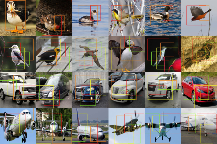
To analyze where Navigator network navigates the model, we draw the navigation regions predicted by Navigator network in Fig. 5. We use red, orange, yellow, green rectangles to denote the top four informative regions proposed by Navigator network, with red rectangle denoting most informative one. It can be seen that the localized regions are indeed informative for fine-grained classification. The first row shows in CUB-200-2011 dataset: we can find that using two regions are able to cover informative parts of birds, especially in the second picture where the color of the bird and the background is quite similar. The second row shows in CUB-200-2011: we can see that the most informative regions of birds are head, wings and main body, which is consistent with the human perception. The third row shows in Stanford Cars: we can find that the headlamps and grilles are considered the most informative regions of cars. The fourth row shows in FGVC Airplane: the Navigator network locates the airplane wings and head, which are very helpful for classification.
5 Conclusions
In this paper, we propose a novel method for fine-grained classification without the need of bounding box/part annotations. The three networks, Navigator, Teacher and Scrutinizer cooperate and reinforce each other. We design a novel loss function considering the ordering consistency between regions’ informativeness and probability being ground-truth class. Our algorithm is end-to-end trainable and achieves state-of-the-art results in CUB-200-2001, FGVC Aircraft and Stanford Cars datasets.
6 Acknowledgments
This work is supported by National Basic Research Program of China (973 Program) (grant no. 2015CB352502), NSFC (61573026) and BJNSF (L172037).
References
- [1] Arbelaez, P., Ponttuset, J., Barron, J., Marques, F., Malik, J.: Multiscale combinatorial grouping. In: CVPR. pp. 328–335 (2014)
- [2] Berg, T., Belhumeur, P.N.: Poof: Part-based one-vs.-one features for fine-grained categorization, face verification, and attribute estimation. In: CVPR (2013)
- [3] Branson, S., Horn, G.V., Belongie, S., Perona, P.: Bird species categorization using pose normalized deep convolutional nets. In: BMVC (2014)
- [4] Burges, C., Shaked, T., Renshaw, E., Lazier, A., Deeds, M., Hamilton, N., Hullender, G.: Learning to rank using gradient descent. In: ICML. pp. 89–96 (2005)
- [5] Cai, S., Zuo, W., Zhang, L.: Higher-order integration of hierarchical convolutional activations for fine-grained visual categorization. In: ICCV (Oct 2017)
- [6] Cao, Z., Qin, T., Liu, T.Y., Tsai, M.F., Li, H.: Learning to rank:from pairwise approach to listwise approach. In: ICML. pp. 129–136 (2007)
- [7] Carreira, J., Sminchisescu, C.: CPMC: Automatic Object Segmentation Using Constrained Parametric Min-Cuts. IEEE Computer Society (2012)
- [8] Chai, Y., Lempitsky, V., Zisserman, A.: Symbiotic segmentation and part localization for fine-grained categorization. In: ICCV. pp. 321–328 (2013)
- [9] Cossock, D., Zhang, T.: Statistical analysis of bayes optimal subset ranking. IEEE Transactions on Information Theory 54(11), 5140–5154 (2008)
- [10] Dalal, N., Triggs, B.: Histograms of oriented gradients for human detection. In: CVPR. pp. 886–893 (2005)
- [11] Endres, I., Hoiem, D.: Category independent object proposals. In: ECCV. pp. 575–588 (2010)
- [12] Fu, J., Zheng, H., Mei, T.: Look closer to see better: Recurrent attention convolutional neural network for fine-grained image recognition. In: CVPR
- [13] Gavves, E., Fernando, B., Snoek, C.G.M., Smeulders, A.W.M., Tuytelaars, T.: Fine-grained categorization by alignments. In: ICCV. pp. 1713–1720 (2014)
- [14] Girshick, R., Donahue, J., Darrell, T., Malik, J.: Rich feature hierarchies for accurate object detection and semantic segmentation. In: CVPR. pp. 580–587 (2014)
- [15] Gosselin, P.H., Murray, N., Jégou, H., Perronnin, F.: Revisiting the fisher vector for fine-grained classification. Pattern Recognition Letters 49, 92–98 (2014)
- [16] He, K., Zhang, X., Ren, S., Sun, J.: Spatial pyramid pooling in deep convolutional networks for visual recognition. TPAMI 37(9), 1904–16 (2015)
- [17] He, K., Zhang, X., Ren, S., Sun, J.: Deep residual learning for image recognition. In: CVPR. pp. 770–778 (2016)
- [18] Herbrich, R.: Large margin rank boundaries for ordinal regression. Advances in Large Margin Classifiers 88 (2000)
- [19] Jaderberg, M., Simonyan, K., Zisserman, A., kavukcuoglu, k.: Spatial transformer networks. In: NIPS, pp. 2017–2025 (2015)
- [20] Jie, Z., Liang, X., Feng, J., Jin, X., Lu, W., Yan, S.: Tree-structured reinforcement learning for sequential object localization. In: NIPS, pp. 127–135 (2016)
- [21] Konda, V.R.: Actor-critic algorithms. Siam Journal on Control and Optimization 42(4), 1143–1166 (2002)
- [22] Krause, J., Jin, H., Yang, J., Fei-Fei, L.: Fine-grained recognition without part annotations. In: CVPR (June 2015)
- [23] Krause, J., Stark, M., Jia, D., Li, F.F.: 3d object representations for fine-grained categorization. In: ICCV Workshops. pp. 554–561 (2013)
- [24] Krizhevsky, A., Sutskever, I., Hinton, G.E.: Imagenet classification with deep convolutional neural networks. In: NIPS. pp. 1097–1105 (2012)
- [25] Lam, M., Mahasseni, B., Todorovic, S.: Fine-grained recognition as hsnet search for informative image parts. In: CVPR (July 2017)
- [26] Li, Z., Yang, Y., Liu, X., Zhou, F., Wen, S., Xu, W.: Dynamic computational time for visual attention. In: ICCV (Oct 2017)
- [27] Lin, T.Y., Dollar, P., Girshick, R., He, K., Hariharan, B., Belongie, S.: Feature pyramid networks for object detection. In: CVPR (July 2017)
- [28] Lin, T.Y., RoyChowdhury, A., Maji, S.: Bilinear cnn models for fine-grained visual recognition. In: ICCV (2015)
- [29] Liu, J., Kanazawa, A., Jacobs, D., Belhumeur, P.: Dog breed classification using part localization. In: ECCV. pp. 172–185 (2012)
- [30] Liu, T.Y.: Learning to rank for information retrieval. Found. Trends Inf. Retr. 3(3), 225–331 (Mar 2009)
- [31] Liu, W., Anguelov, D., Erhan, D., Szegedy, C., Reed, S., Fu, C.Y., Berg, A.C.: Ssd: Single shot multibox detector. In: ECCV. pp. 21–37 (2016)
- [32] Liu, X., Xia, T., Wang, J., Lin, Y.: Fully convolutional attention localization networks: Efficient attention localization for fine-grained recognition. CoRR (2016)
- [33] Long, J., Shelhamer, E., Darrell, T.: Fully convolutional networks for semantic segmentation. CVPR (Nov 2015)
- [34] Lowe, D.G.: Distinctive image features from scale-invariant keypoints. IJCV (2004)
- [35] Maji, S., Kannala, J., Rahtu, E., Blaschko, M., Vedaldi, A.: Fine-grained visual classification of aircraft. Tech. rep. (2013)
- [36] Moghimi, M., Belongie, S., Saberian, M., Yang, J., Vasconcelos, N., Li, L.J.: Boosted convolutional neural networks. In: BMVC. pp. 24.1–24.13 (2016)
- [37] Redmon, J., Divvala, S., Girshick, R., Farhadi, A.: You only look once: Unified, real-time object detection. In: CVPR. pp. 779–788 (2016)
- [38] Ren, S., He, K., Girshick, R., Sun, J.: Faster r-cnn: Towards real-time object detection with region proposal networks. In: NIPS. pp. 91–99 (2015)
- [39] Russakovsky, O., Deng, J., Su, H., Krause, J., Satheesh, S., Ma, S., Huang, Z., Karpathy, A., Khosla, A., Bernstein, M., Berg, A.C., Fei-Fei, L.: ImageNet Large Scale Visual Recognition Challenge. IJCV 115(3), 211–252 (2015)
- [40] Sermanet, P., Eigen, D., Zhang, X., Mathieu, M., Fergus, R., Lecun, Y.: Overfeat: Integrated recognition, localization and detection using convolutional networks. Arxiv (2013)
- [41] Uijlings, J.R., Sande, K.E., Gevers, T., Smeulders, A.W.: Selective search for object recognition. IJCV 104(2), 154–171 (2013)
- [42] Wah, C., Branson, S., Welinder, P., Perona, P., Belongie, S.: The Caltech-UCSD Birds-200-2011 Dataset. Tech. rep. (2011)
- [43] Wang, D., Shen, Z., Shao, J., Zhang, W., Xue, X., Zhang, Z.: Multiple granularity descriptors for fine-grained categorization. In: ICCV. pp. 2399–2406 (2015)
- [44] Xia, F., Liu, T.Y., Wang, J., Li, H., Li, H.: Listwise approach to learning to rank: theory and algorithm. In: ICML. pp. 1192–1199 (2008)
- [45] Xie, L., Tian, Q., Hong, R., Yan, S.: Hierarchical part matching for fine-grained visual categorization. In: ICCV. pp. 1641–1648 (2013)
- [46] Zhang, N., Donahue, J., Girshick, R., Darrell, T.: Part-based rcnn for fine-grained detection. In: ECCV (2014)
- [47] Zhang, X., Xiong, H., Zhou, W., Lin, W., Tian, Q.: Picking deep filter responses for fine-grained image recognition. In: CVPR (June 2016)
- [48] Zhao, B., Wu, X., Feng, J., Peng, Q., Yan, S.: Diversified visual attention networks for fine-grained object classification. Trans. Multi. 19(6), 1245–1256 (Jun 2017)
- [49] Zheng, H., Fu, J., Mei, T., Luo, J.: Learning multi-attention convolutional neural network for fine-grained image recognition. In: ICCV (Oct 2017)