Modeling the Role of Gap Junction Transport Characteristics in the Action Potential Propagation

Abstract

We generalize the Cable Model to describe the transport characteristics of the gap junctions coupling adjacent cells in the heart muscle. Our model takes into account recent experimental information about the time dependence of the junctional current and modifies the connections between cells. It can be used with whatever excitable model is used to represent the cell. We show that by modulating the gap junction transport characteristics, it is possible to either suppress or produce meandering of spiral waves, a state associated with cardiac arrhythmia.

1 Introduction

Spirals are generic structures in extended nonequilibrium systems. They are typical of many reaction-diffusion systems, and have been directly visualized in the heart muscle associated with reentrant wave fronts [1].

The spiral wave dynamics was numerically studied in both isotropic and anisotropic media, and limited or unlimited geometries [2]-[6]. If the spiral tip rotates around a stationary region, the activation wave front will follow the same path from one complete reentrant cycle to the next, and the associated ECG will exhibit a monomorphic pattern. When the tip meanders, the activation sequence from one reentrant cycle to the next will be different and the associated ECG can exhibit polymorphic patterns. Polymorphic patterns appear in the ECG related to ionic channel blockade, regions of refractory tissue, intracellular calcium instabilities, etc [1][7]-[10].

More recently the challenge of the role of gap junctions in electrical wave propagation has encourage investigations about the proarrhythmic effects of reduced intercellular coupling[11]-[15]. Adjacent cells are coupled by the myocardial gap junction channels, which transmit the intercellular voltage gradients and allow the action potential propagation. Disruption of the gap junction membrane structures terminates the transfer of cardiac action potential across an electrically unexcitable gap. Severe gap junctional uncoupling not only drastically reduces conduction velocity, but also further results in meandering activation wavefronts.[16],[17]

Simulations are usually made in the so-called Cable Model [2],[3][18]-[20] where the gap junction coupling is introduced as a constant conductance. However, gap junctions are not passive but dynamic pores that allow ions to pass from one cell to the next.

Experimental information also indicates that junctional current decays exponentially when a constant voltage difference is applied across the junction (pulse protocol).[21]-[26]

Other studies have considered the dynamic nature of the gap junctions. Although these studies demostrated the significant dynamics that can occur in the gap junction for the cases near decremental propagation and conduction block, results did not deviate qualitatively from those observed with the more classical representation of gap junctions as constant resistors.[27]

In the present work, we generalize the Cable Model by introducing the above-mentioned experimental finding and show that by modulating the gap junction transport characteristics, it is possible either to suppress or to produce meandering of spiral waves, a state associated with cardiac arrhythmia.

2 The Model

The origin of the action potential $V_{m}$ in an isolated cell lies in the movement of ions throughout the cell membrane characterized by a capacitance $C_{m}$. The process is described by

$$\frac{\partial V_{m}}{\partial t}=-\frac{I_{ion}(t)}{C_{m}}$$ (1)

where $I_{ion}$ is the total ionic current, produced by the transport of different ions throughout a number of ionic channels, and other interchange mechanisms[28]. A value of $I_{ion}<0$ represents the entrance of positive ions into the cell and an increase of $V_{m}$, i.e., a depolarization of the cell. A reduction of $V_{m}$ (repolarization of the cell) is produced by a value of $I_{ion}>0$, representing the outgoing of positive ions from the cell. In general, $I_{ion}$ is the sum of outgoing and incoming currents ($I_{x}$), characterized by different magnitudes and dependences on $V_{m}$

$$I_{ion}=\sum_{x=1}^{n}I_{x}$$ (2)

A number of dynamic models have been used to derive $I_{ion}$.

The modification proposed in the present work affects the connections between cells and therefore it can be applied whatever dynamic model is used to express $I_{ion}$.

In the Cable Model the propagation of $V_{m}$ wave fronts is schematized in Figure $1a$. An excitable model describes a membrane cell, and several membrane cells are connected through resistors. The resistor grid represents both the intracellular medium and the intercellular channels, and the extracellular medium is assumed to have a negligible resistance compared to the intracellular space.

The total cell current $I_{t}$ is given by

$$C_{m}\frac{\partial V_{m}}{\partial t}+I_{ion}=-I_{t}$$ (3)

while the total intercellular current $I_{i}=I_{ix}+I_{iy}$ is given by

$$g_{ix}\frac{\partial V_{m}}{\partial x}+g_{iy}\frac{\partial V_{m}}{\partial y}=I_{i}$$ (4)

where $g_{ix}$ and $g_{iy}$ indicate both the intracellular and the intercellular conductivities, and an anisotropic medium is assumed. Note that $g_{ix}^{-1}$ and $g_{iy}^{-1}$ are extended resistivities, i.e., $\left[g_{ix}^{-1}\right]=\left[g_{iy}^{-1}\right]=\Omega/m$.

Furthermore, the total cell current per unit length is given by

$$\frac{\partial I_{ix}}{\partial x}+\frac{\partial I_{iy}}{\partial y}\simeq\frac{\Delta I_{ix}}{\Delta x}+\frac{\Delta I_{iy}}{\Delta y}=-\left(\frac{I_{t1}}{\Delta x}+\frac{I_{t2}}{\Delta y}\right)=-\frac{I_{t}}{\Delta}$$ (5)

where $\Delta x=\Delta y=\Delta$ is the unit length.

Therefore,

$$g_{ix}\frac{\partial^{2}V_{m}}{\partial x^{2}}+g_{iy}\frac{\partial^{2}V_{m}}{\partial y^{2}}=C_{m}\frac{\partial V_{m}}{\partial t}+I_{ion}$$ (6)

where $\Delta$ has been omitted on the rigth-hand side for simplicity.

We note that the scale change

$$X = x$$ (7)

$$Y = \sqrt{\frac{g_{ix}}{g_{iy}}}y$$ (8)

eliminates the anisotropy effect in Eq. $6$. The quantity $g/C_{m}=D$ defines a diffusion coefficient.

But gap junction channels have time and $V_{i}$-dependent inactivation properties that are dependent on the transjunctional or intercellular voltage $V_{i}$. Experiments have been made on conexin 40  and conexin 43 gap junctions, and the intercellular current $I_{i}$ exponentially decays in time with time constants depending on $V_{i}$.

In these experiments a constant transjunctional voltage $V_{i}$ is applied using a pulse protocol where a $V_{i}$ pulse is repeated five times and the ensemble average $I_{i}$ was fitted with an exponentially decaying function to determine the decay time constants. The reciprocal of the decaying time constants $(\tau)$ from $4$ to $10$ experiments at each $V_{i}$ were plotted fitted with the general exponential expression [21]-[23]

$$\frac{1}{\tau}=A^{0}\exp(\left|V_{i}\right|/v_{0})$$ (9)

where $A^{0}$and $v_{0}$ are constants.

These experimental findings indicate that the Cable Model describing the intercellular channels as resistors must be improved and time variations of $I_{i}$ must be explicitly considered.

The modification proposed in the present work is schematized in Figure 1b.

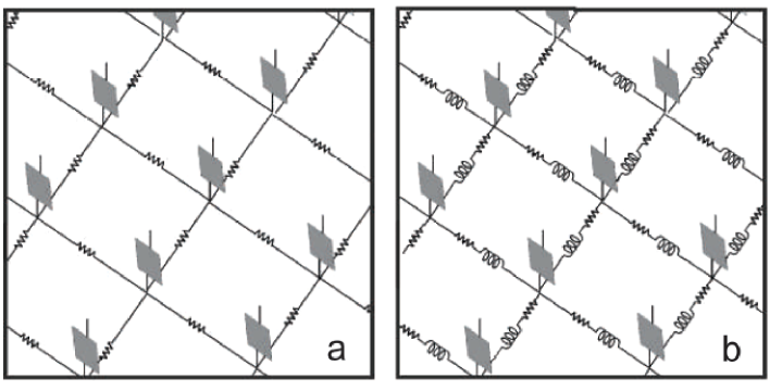
Figure 1: (a) Cable Model scheme: each gray square represents an excitable model describing the membrane cell, and several membrane cells are connected through resistors; (b) Generalized Cable Model scheme: the membrane cells are connected through resistors and inductances (recovery constant).

We consider the intercellular current $I_{i}$ as a recovery variable and write Eq. 4 as

$$\frac{\partial V_{m}}{\partial x} = \frac{1}{g_{ix}}I_{ix}+L_{ix}\frac{\partial I_{ix}}{\partial t}$$ (10)

$$\frac{\partial V_{m}}{\partial y} = \frac{1}{g_{iy}}I_{iy}+L_{iy}\frac{\partial I_{iy}}{\partial t}$$ (11)

where $L_{ix}$ and $L_{iy}$ are recovery constants and

$$\frac{1}{g_{ix}}=A_{0}\exp(\left|V_{ix}\right|/v_{c})$$ (12)

with $A_{0}$ and $v_{c}$ constants, and

$$V_{ix}=\frac{\partial V_{m}}{\partial x}$$ (13)

and identical equations in the $y$ direction.

Note that if $V_{ix}$ is constant $I_{i}$ is an exponentially decaying function with a decay time constant depending of $V_{ix}$, as was experimentally observed.

Assuming that $I_{ix}$ and $I_{iy}$ are analytical functions (i.e., $\frac{\partial}{\partial x}(\frac{\partial I_{ix}}{\partial t})=\frac{\partial}{\partial t}(\frac{\partial I_{iy}}{\partial x})$), with the approximations $(g_{ix}v_{0})^{-1}<<1$, $(g_{iy}v_{0})^{-1}<<1$, and Eq. 3 we obtain

$$C_{m}\frac{\partial V_{m}}{\partial t}+I_{ion}=-\left(I_{tx}+I_{ty}\right)$$ (14)

$$\frac{\partial I_{tx}}{\partial t}+\frac{1}{g_{ix}L_{ix}}I_{tx} = -\frac{1}{L_{ix}}\frac{\partial^{2}V_{m}}{\partial x^{2}}$$ (15)

$$\frac{\partial I_{ty}}{\partial t}+\frac{1}{g_{iy}L_{iy}}I_{ty} = -\frac{1}{L_{iy}}\frac{\partial^{2}V_{m}}{\partial y^{2}}$$ (16)

$$I_{t} = I_{tx}+I_{ty}$$ (17)

where $\Delta$ was omitted for simplicity on the lef-hand side of Eqs. $15-16$, as in Eq. $6$. This Generalized Cable Model (GCM) reduces to the former one (Eqs. $3$ and $4$) under the following conditions:

(i) Stationary state for $I_{ix}$ and $I_{iy}$.

(ii) Isolated cells (i.e., $\frac{\partial^{2}V_{m}}{\partial x^{2}}=\frac{\partial^{2}V_{m}}{\partial y^{2}}=0$) at $t\rightarrow\infty$($I_{ti}\rightarrow 0$, $i=1,2$).

3 Results

We explored the GCM by using the cellular Barkley model to describe the time variation of $I_{ion}$ as well as its dependences on $V_{m}$[29]. The Barkley model is perhaps one of the simplest cellular models showing excitability.The cell is represented by an equivalent circuit containing three elements connected in parallel: a capacitor representing the cellular membrane, a variable resistor describing the ionic channels and an inductance in series with a resistor representing the intracellular medium. The Barkley model is extended by using the Cable Model with a constant diffusion coefficient, and it is written as

$$\frac{\partial u}{\partial t} = \varepsilon^{-1}u(1-u)\left[u-(v+b)/a\right]+D\nabla^{2}u$$ (18)

$$\frac{\partial v}{\partial t} = u-v$$ (19)

where $u$ and $v$ are the dimensionless versions of $V_{m}$ and $I_{ion}$ respectively, $D$ is the diffusion coefficient, and $a$, $b$ and $\varepsilon$ are parameters to model the nonlinear dependence of $I_{ion}$ on $V_{m}$.

The space parameter of the Barkley model is shown in Figure 2 (modified from Ref [29]). Stable 2D spiral waves are found in numerical simulations inside the white region, and meandering of spiral waves takes place in the MS region. The 2D medium does not support excitation waves in region NW, is subexcitable in region SE, and is bistable in region BI.

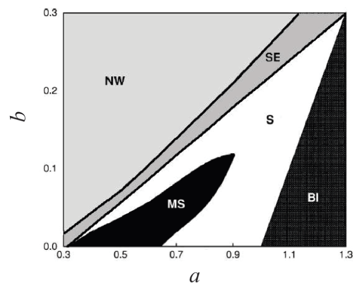
Figure 2: Phase diagram of the spatially extended Barkley model (modified from Ref: 29). MS: meandering of spirals, S: stable spirals, SE: subexcitable zone, NW: no waves, BI: bistability.

In the present work we extend the Barkley model with the GCM and write

$$\frac{\partial u}{\partial t} = \varepsilon^{-1}u(1-u)\left[u-(v+b)/a\right]-\sum_{j=1}^{2}w_{j}$$ (20)

$$\frac{\partial v}{\partial t} = u-v$$ (21)

$$\frac{\partial w_{j}}{\partial t} = -k_{j}w_{j}-k_{j}D\frac{\partial^{2}u}{\partial x_{j}^{2}}$$ (22)

where $w$ is the dimensionless version of $I_{t}$, and the subindex $j=1,2$ considers the two Cartesian directions in a two-dimensional tissue. Note that we do not explicitly reduce a cellular model to its dimensionless form. This will depend on the model used and we want to show only how two cells should be coupled taking into account the basic properties of the gap junctions. We used the model constants ($A$ and $B$ in Eq. 23) to characterized its dynamical behaviour in this new parametric space.

$k_{j}$ is given by

$$k_{j}=A\exp(u_{j}^{2}/B)$$ (23)

with

$$u_{j}=\frac{\partial u}{\partial x_{j}}$$ (24)

and where $A$ and $B$ are constants related with $A_{0}$ and $\nu_{c}$.

Note the anisotropy of $w_{j}$. Equation 23 takes into account the experimentally observed dependence on $V_{i}$ of the decay time constants in the time dependence of $I_{i}$ (see Eq. 9). In this paper a quadratic dependence was introduced (instead of a $\left|V_{i}\right|-$dependence) to preserve the even nature of the function but to avoid the nondifferentiable point at $V_{i}=0$.

The model of Eqs. 20-22 reduces to the original Barkley model in the following situations:

(i) Adiabatic conditions for $w_{j}$, i.e. $\frac{\partial w_{j}}{\partial t}=0.$

(ii) No diffusion of $u$ at $t\rightarrow\infty$ (i. e., $w_{j}\rightarrow 0$).

In Eq. 23 the new parameters $A$ and $B$ regulate the transport of different ions throughout the gap junction channels, and we show that they determine the existence of either stable wave fronts (associated with a normal electrical behavior of the heart) or meandering (associated with arrhythmic behavior).

Figure 3 shows a characterization of our model in the $A-B$ parameter space. Simulations were performed with $k_{j}D=1$, $\varepsilon=0.02$, $a=0.7$, $b=0.05$. For these parameter values the original Barkley model (with $D=1$) exhibits meandering of spirals. In the MS region in Fig. 3 we obtain meandering of spirals, while in the S region there are stable wave fronts. For $1/B=0$ (see Figure 3), the problem reduces to one with constant diffusion $D=1/A$. In particular for $A=1$ ($D=1$) we obtain stable wave fronts, differing from the original Barkley model where meandering is obtained.

Therefore, the introduction of $w_{j}$ in the GCM produces nontrivial modifications in the dynamic behavior of the system.

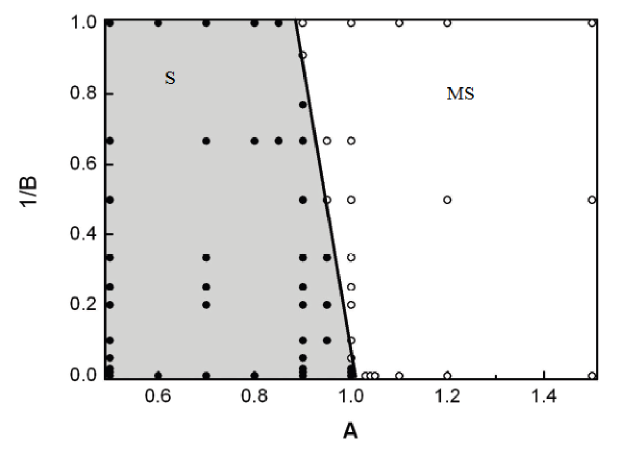
Figure 3: Phase diagram of the modified spatially extended Barkley model. MS: meandering of spirals, S: stable spirals. Simulations were performed with $k_{j}D=1$, $\varepsilon=0.02$, $a=0.7$, $b=0.05$.

4 Conclusions

The results presented in this work show that the modification of the gap junction transport properties can either suppress or favor the development of spiral meandering.

Our conclusions are in agreement with experimental evidence showing that severe gap junctional uncoupling results in meandering activation wavefronts[16],[17].

Of course the existence of meandering also depends on the cellular model used in the simulation and it can be due to a number of other mechanisms such as alterations in the excitability, anisotropy, etc.

The modelling of the gap junction transport properties performed in this work explicitly introduces the exponential decaying of the intracellular current $I_{t}$, by considering it as a recovery variable. In this sense our model differs from other models that consider time and voltage dependent conductances.[30],[31]

Alternatively, gap junctions can be considered as channels which are ”gated” in a voltage-sensitive manner, so that the channels open and close in response to the membrane potential. These gates can be represented by using the Hodgkin-Huxley formalism, in which the conductance term is decomposed into the product of a maximal conductance term and one or more separate normalized variables that represent the probability of finding the channel open. These variables follow their own differential equations. The most common formulation for a gating variable $s_{i}$ is

$$\frac{\partial s_{i}}{\partial t}=(s_{0}-s)/ts$$ (25)

where $s_{0}$ is the voltage dependent steady-state value of the gate and $t_{s}$ is the voltage-dependent time constant of the gate.

This formalism applied to $I_{t}$ naturally leads to equations similar to those used in the present work.

Acknowledgments

This work was supported by the Consejo Nacional y Ciencia y Tecnolog s (CONICET), Agencia Nacional de Promoci n Cient fica y Tecnol gica (ANPCyT) and Universidad Nacional de La Plata (UNLP).

References

- [1] C. F. Starmer, D. N. Romashko, R. S. Reddy, Y. I. Zilberter, J. Starobin, A. O. Grant, and V. I. Krinsky, Circulation 92, 595 (1995).
- [2] D. Olmos, B. D. Shizgal, Phys. Rev. E 77; 31918 (2008).
- [3] F. Siso-Nadal, N. F. Otani, R. F. Gilmour, Jr, J. J. Fox, Phys. Rev. E 78, 31925 (2008).
- [4] F. H. Fenton, E. M. Cherry, A. Karma, W-J. Rapel, Chaos 15, 13502 (2005).
- [5] E. M. Cherry, H. S. Greenside, C. S. Henriquez, Chaos 13, 853 (2003).
- [6] J. Dou, L. Xia, Y. Zhang, G. Shou, Q. Wei, F. Lin, S. Crozier, Phys. Med, Biol. 54, 353 (2009).
- [7] Z. Qu, Y. Shiferaw, J. N Weiss, Phys. Rev. 75, 011927 (2007).
- [8] Y. Xie, G. Hu, D. Sato, J. N. Weiss, A. Garfinkel, Z. Qu, Phys Rev. Lett. 99, 118101 (2007).
- [9] X. Zhao, Phys. Rev. E 78, 11902 (2008).
- [10] M Kawatou, H. Masumoto, H.Fukushima, G.Morinaga, R.Sakata, T. Ashihara, J. K. Yamashita, Nature Communicationsvolume 8, Article number: 1078 (2017).
- [11] S. M. Taffet, J. Jalife, Circ. Res. 94, 4 (2004).
- [12] J. K. Hennan, R. E. Swillo, G. A. Morgan, Jr J. C. Keith, R. G. Schaub, R. P. Smith, et al., J. Pharmacol. Exp. Ther. 317, 236 (2006).
- [13] A. L. Wit, H. S. Duffy,Am J Physiol Heart Circ Physiol 294, H16 (2008).
- [14] G. Laurent, H. Leong-Poi, I. Mangat, G. W. Moe, X. Hu, P. P.-S. So, E. Tarulli, A. Ramadeen, E. I. Rossman, J. K. Hennan, P. Dorian, Circulation: Arrhythmia and Electrophysiology. 2, 171 (2009).
- [15] N. R. Jorgensen, S. C. Teilmann, Z. Henriksen, E. Meier, S. S. Hansen, J. E. Jensen, O. H. Sorensen, J. S. Petersen, Endocrinology. 146, 4745 (2005).
- [16] S. Rohr, J. P. Kucera, A. G. Kl ber, Circ. Res. 83, 781 (1998).
- [17] S. Rohr, Cardiovascular REs. 62, 309 (2004).
- [18] D. Sato, Y. Shiferaw, A. Garfinkel, J. N. Weiss, Z. Qu, A. Karma, Circ. Res. 99, 520 (2006).
- [19] J. Kneller, J. Kalifa, R. Zou, A. V. Zaitsev, M. Warren, O. Berenfeld, E. J. Vigmond, L. J. Leon, S. Nattel, J. Jalife, Circ. Res. 96, e357 (2005).
- [20] T. Krogh-Madsen, D. J. Christini, Phys. Rev. E 77, 11916 (2008).
- [21] J. E. Saffitz, J. G. Laing, K. A. Yamada , Circ. Res. 86, 723 (2000).
- [22] X. Lin, M. Crye, R. D. Veenstra, Circ. Res. 93, e63 (2003).
- [23] X. Lin, R. D. Veenstra, Am. J. Physiol. Heart Circ. Physiol. 286, H1726 (2004).
- [24] S. R. Kaplan, J. J. Gard, N. Protonotarios, A. Tsatsopoulou, C. Spiliopoulou, A. Anastasakis, et al., Heart Rhythm 1, 3 (2004).
- [25] U. Wetzel, A. Boldt, J. Lauschke, J. Weigl, P. Schirdewahn, A. Dorszewski, N. Doll, G. Hindricks, S. Dhein, H. Kottkamp, Heart 91, 166 (2005).
- [26] X. Lin, J. Gemel, E. C. Beyer, R. D, Veenstra, Am. J. Physiol. Heart Circ Physiol.288, H1113 (2005).
- [27] A. P. Henriquez, R. Vogel, B. J. Muller-Borer, C. S. Henriquez, R. Weingart, W. E. Cascio, Biophys. J. 81, 2112 (2001).
- [28] D. P. Zipes, J. Jalife, Cardiac Electrophysiology: From Cell to Bedside, 4th ed. Elsevier Inc., New York, New York, USA.
- [29] S. Alonso, R. K hler, A. S. Mikhailov and F. Sagu s, Phys. Rev. E 70, 056201 (2004).
- [30] R.H. Clayton, O. Bernus b, E.M. Cherry, H. Dierckx, F.H. Fenton, L. Mirabella, A.V. Panfilov, F.B. Sachse, G. Seemann, H. Zhang. Progress in Biophysics and Molecular Biology 104 (2011) 22-48.
- [31] N. A. Trayanova, Circ Res. 2011 Jan 7; 108(1): 113–128.