Unbiased Predictive Risk Estimation of the Tikhonov Regularization Parameter.

Abstract.

The truncated singular value decomposition may be used to find the solution of linear discrete ill-posed problems in conjunction with Tikhonov regularization and requires the estimation of a regularization parameter that balances between the sizes of the fit to data function and the regularization term. The unbiased predictive risk estimator is one suggested method for finding the regularization parameter when the noise in the measurements is normally distributed with known variance. In this paper we provide an algorithm using the unbiased predictive risk estimator that automatically finds both the regularization parameter and the number of terms to use from the singular value decomposition. Underlying the algorithm is a new result that proves that the regularization parameter converges with the number of terms from the singular value decomposition. For the analysis it is sufficient to assume that the discrete Picard condition is satisfied for exact data and that noise completely contaminates the measured data coefficients for a sufficiently large number of terms, dependent on both the noise level and the degree of ill-posedness of the system. A lower bound for the regularization parameter is provided leading to a computationally efficient algorithm. Supporting results are compared with those obtained using the method of generalized cross validation. Simulations for two-dimensional examples verify the theoretical analysis and the effectiveness of the algorithm for increasing noise levels, and demonstrate that the relative reconstruction errors obtained using the truncated singular value decomposition are less than those obtained using the singular value decomposition.
This is a pre-print of an article published in BIT Numerical Mathematics. The final authenticated version is available online at: https://doi.org/10.1007%2Fs10543-019-00762-7

Convergence with increasing rank approximations of the Singular Value Decomposition

1. Introduction

We consider the solution of $A\mathbf{x}\approx\mathbf{b}$, or $A\mathbf{x}\approx\mathbf{{\mathbf{b}}_{\text{true}}}+\bm{\eta}=\mathbf{b}$ for noise (measurement error) $\bm{\eta}$, where $A\in\mathcal{R}^{m\times n}$ is ill-conditioned, and the system of equations arises from the discretization of an ill-posed inverse problem that may be over or under determined. The general Tikhonov regularized linear least squares problem

(1) $$\mathbf{x}^{*} =\textnormal{arg}\min_{\mathbf{x}}\{\|A\mathbf{x}-\mathbf{b}\|_{W_{\mathbf{b}}}^{2}+\|D(\mathbf{x}-{\mathbf{x}}_{0})\|^{2}_{W_{\mathbf{x}}}\},$$

is a well-accepted approach for finding a smooth solution $\mathbf{x}$. Here ${\mathbf{x}}_{0}$ is given prior information, possibly the mean of $\mathbf{x}$, $W_{\mathbf{b}}$ and $W_{\mathbf{x}}$ are weighting matrices on the data fidelity and regularization terms, resp., and $D$ is an optional regularization operator. Often $D$ is imposed as a spatial differential operator, controlling the size of the derivative(s) of $\mathbf{x}$, but then (1) can be brought into standard form in which $D$ is replaced by $I$, [5, 21]. Further, (1) can be rewritten in terms of a new variable $\mathbf{y}=\mathbf{x}-{\mathbf{x}}_{0}$. The weighted norm is defined by $\|\mathbf{x}\|^{2}_{W}:=\mathbf{x}^{T}W\mathbf{x}$ and we use the notation $\mathbf{m}\sim\mathcal{N}(\bm{m}_{0},C_{\mathbf{m}})$ for random vector $\mathbf{m}$ normally distributed with expected value $E(\bm{m})=\bm{m}_{0}$ and covariance matrix $C_{\mathbf{m}}$; $E(\cdot)$ is used to denote expected value. When $\bm{\eta}\sim\mathcal{N}(0,C_{\mathbf{b}})$, then $W_{\mathbf{b}}=C_{\mathbf{b}}^{-1}$ whitens the noise, i.e. $W_{\mathbf{b}}^{1/2}\bm{\eta}\sim\mathcal{N}(0,I)$. Matrix $W_{\mathbf{x}}=C_{\mathbf{x}}^{-1}$ can serve similarly as a prior on the inverse covariance of the noise in $D\mathbf{y}$. Using $W_{\mathbf{x}}=\alpha^{2}I$, as will be assumed here, corresponds to assuming the posterior distribution $D\mathbf{y}\sim\mathcal{N}(0,\alpha^{-2})$, see e.g. [27]. Here we discuss the solution of (1) with ${\mathbf{x}}_{0}=0$, $D=I$, $W_{\mathbf{x}}=\alpha^{2}I$, $W_{\mathbf{b}}=I$ and explicitly assume common variance, $\sigma^{2}$, in the noise, $\bm{\eta}\sim\mathcal{N}(0,\sigma^{2}I)$.

While solutions of (1) have been extensively studied, e.g. [17, 21, 22, 41] there is still much discussion concerning the selection of $W_{\mathbf{x}}$ even for the single parameter case, $W_{\mathbf{x}}=\alpha^{2}I$. Suggested techniques include, among others, using the Morozov discrepancy principle (MDP) which assumes that the solution should be found within some prescribed $\chi^{2}$ noise estimate [29], balance of the terms in (1) using the L-curve [21], the quasi-optimality condition [3, 15, 16] and minimization of the generalized cross validation (GCV) function [11] or of the statistically motivated Unbiased Predictive Risk Estimator (UPRE) [33, 41]. Of these the MDP, GCV and UPRE approaches are all a posteriori estimators, the MDP on the $\chi^{2}$ distribution of the predicted residual, the GCV through its derivation as a leave one out procedure to minimize the predictive error and the UPRE as an estimator of the minimum predictive risk of the solution. There is an extensive discussion of these methods in the standard literature e.g. [21, 22, 41] and many more are compared in [4]. We do not replicate that discussion here, rather we focus on the UPRE parameter choice method. The UPRE method has a firm theoretical foundation, is robust, and has been extensively applied in practical applications, [1, 18, 25, 27, 35, 37, 38, 39, 40]. Our analysis extends the approach in [9] which provided bounds on the regularization parameter for finding $\alpha$ using the GCV; the analysis in [30] that examined convergence of the parameter with increasing resolution of the problem via the connection of the continuous and discrete singular value expansions for specific square integrable operators defining $A$; and the discussion in [31] that demonstrated the relationship of the regularization parameter obtained when using the LSQR Krylov method for large scale problems. Moreover, our interest in the UPRE, instead of the MDP, arises because the UPRE depends only on the underlying knowledge of the noise distribution, whereas the MDP also introduces a secondary tolerance factor on the satisfaction of the $\chi^{2}$ distribution, which is often needed to limit over smoothing of the solutions, [2].

Throughout we use the Singular Value Decomposition (SVD) $A=U\Sigma V^{T}$, [12], with columns $\mathbf{u}_{i}$ and $\mathbf{v}_{i}$ of orthonormal $U$ and $V$ respectively, and where the singular values $\sigma_{i}$ of $A$ are ordered on the principal diagonal of $\Sigma$, from largest to smallest. We assume that the matrix $A$ has effective numerical rank $r$; $\sigma_{r}>0$, and $\sigma_{i}$, $i>r$ is effectively zero as determined by the machine precision. In terms of the SVD components, the solution of (1) is given by

(2) $$\mathbf{x}^{*}=\sum_{i=1}^{r}\frac{\sigma_{i}^{2}}{\sigma_{i}^{2}+\alpha^{2}}\frac{\mathbf{u}_{i}^{T}\mathbf{b}}{\sigma_{i}}\mathbf{v}_{i}=\sum_{i=1}^{r}\gamma_{i}(\alpha)\frac{\mathbf{u}_{i}^{T}\mathbf{b}}{\sigma_{i}}\mathbf{v}_{i},\quad\gamma_{i}(\alpha)=\frac{\sigma_{i}^{2}}{(\sigma_{i}^{2}+\alpha^{2})}.$$

The filter functions are $\gamma_{i}(\alpha)$ and the given expansion applies, replacing $r$ by $k$, when $A$ is approximated by the TSVD, $A_{k}=U_{k}\Sigma_{k}V_{k}^{T}$. Throughout we use the subscript $k$ to indicate variables associated with this rank $k$ approximation, for example regularization parameter $\alpha_{k}$ indicates the regularization parameter used for the $k$-term TSVD. Further, the use of the SVD for $A$ provides useful insights on how the UPRE, and other methods, can be implemented when solving (1). Here we will show that the minimization of the underlying UPRE function is efficient and robust with respect to the $k-$term truncated singular value decomposition (TSVD). Moreover, there is a resurgence of interest in using a TSVD solution for the solution of ill-posed problems due to the increased feasibility of finding a good approximation of a dominant singular subspace even for large scale problems by using techniques from randomization, e.g. [7, 8, 13, 26, 28, 32]. Thus the presented results will be more broadly relevant for efficient estimates of an approximate TSVD using these modern techniques applied for large scale problems, for which it is not feasible to find the full SVD expansion; necessarily $k<<r$.

Overview of main contributions. An open source algorithm, Algorithm 1, for efficiently estimating optimal regularization parameters $k_{\mathrm{opt}}$ and $\alpha_{k_{\mathrm{opt}}}$, defined to be the optimal number of terms to use from the TSVD, and the associated regularization parameter, resp., is presented. By optimal we mean that these parameters are optimal in the sense of minimizing the UPRE function. A MATLAB implementation of Algorithm 1 and a $2D$ test case using IR Tools [10] is available at https://github.com/renautra/TSVD_UPRE_Parameter_Estimation. A Python 3.* implementation using NumPy and SciPy is also available and relies on provision of the singular values and coefficients $\mathbf{u}_{i}^{T}\mathbf{b}$. In both cases an estimate for the noise variance in the data is required, as is standard for the UPRE method. The motivation for Algorithm 1 is based on the theoretical results presented in Section 3. These results employ standard assumptions on the degree of ill-posedness of the underlying model and on the noise level in the data, [23]. We briefly review how both the degree of ill-posedness and the noise level impact the choice of regularization parameter $k$, and demonstrate that the noise level is far more restrictive so that in general $k\ll r$. The convergence of $\alpha_{k}$, when found using both UPRE and GCV methods, is illustrated for examples from the Regularization toolbox [20]. The theory presented in Section 3 then leads to Theorems 3.1 and 3.2 which prove a lower bound for $\alpha_{k}$ and that $\alpha_{k}$ converges to $\alpha_{k_{\mathrm{opt}}}$, under the assumption of a unique minimum of the UPRE function. Presented results for image deblurring verify the practicality of Algorithm 1 and demonstrate that the solutions obtained with $k_{\mathrm{opt}}<r$ yield smaller overall relative error than the solutions obtained without truncation of the SVD and $\alpha_{r}$ found using the UPRE method.

The paper is organized as follows: In Section 2 we present background motivating results based on assumptions on the degree of ill-posedness of the problem in Section 2.1, a discussion of numerical rank in Section 2.2, how noise enters into the problem in Section 2.3 and the estimation of the regularization parameter in Section 2.4. The theoretical results providing our main contributions are presented in Section 3. A practical algorithm for estimating $\alpha_{k_{\mathrm{opt}}}$, and hence also $k_{\mathrm{opt}}$, is presented in Section 4 with simulations verifying the analysis and the algorithm for two dimensional cases. Conclusions and future extensions are provided in Section 5.

2. Motivating Results

2.1. Degree of Ill-Posedness

As in [23, Definition 2.42], and subsequently adopted in [21], for the analysis we assume specific decay rates for the singular values dependent on whether the problem is mildly, moderately or severely ill-posed. Suppose that $\zeta$ is an arbitrary constant, then the decay rates are given by

(3) $$\sigma_{i}=\left\{\begin{array}[]{lll}\zeta i^{-\tau}&\frac{1}{2}\leq\tau\leq 1&\text{mild ill conditioning}\\ \zeta i^{-\tau}&\tau>1&\text{moderate ill conditioning,}\\ \zeta\tau^{-i}&\tau>1&\text{severe ill conditioning.}\end{array}\right.$$

Here $\tau$ is a problem dependent parameter and it is assumed that the decay rates hold on average for sufficiently large $i$. Moreover, while defining $\sigma_{i}$ in terms of index $i$, as is consistent with the literature, it will also be convenient to consider the definition in terms of the continuous variable $i$, so that $\sigma_{i+\delta}$ is defined also for non-integer $i+\delta$. For ease, and without loss of generality, we pick the constant $\zeta$ in (3) so that $\sigma_{1}=1$ in all cases. Equivalently we use

(4) $$\sigma_{i}=\left\{\begin{array}[]{lll}i^{-\tau}&\frac{1}{2}\leq\tau\leq 1&\text{mild ill conditioning,}\\ i^{-\tau}&\tau>1&\text{moderate ill conditioning,}\\ \tau^{1-i}&\tau>1&\text{severe ill conditioning,}\end{array}\right.$$

and note the recurrences

$$\sigma_{\ell+1}=\sigma_{\ell}\left\{\begin{array}[]{ll}(\frac{\ell}{\ell+1})^{\tau}&\text{mild or moderate ill conditioning,}\\ \tau^{-1}&\text{severe ill conditioning.}\end{array}\right.$$

2.2. Numerical Rank

The precision of the calculations, as determined by the machine epsilon $\epsilon$, is relevant in terms of the number of singular values that are significant in the calculation. This is dependent on the decay rate parameters of the singular values. We define the effective rank by $r=\mathrm{argmax}\{i:\sigma_{i}>\epsilon\sigma_{1}\}$.

Proposition 2.1.

Assuming the normalization of the singular values as given by (4), the effective numerical rank $r$ is bounded by

(7) $$r<\left\{\begin{array}[]{ll}\epsilon^{-1/\tau}&\text{mild / moderate decay, }\\ 1-\frac{\log\epsilon}{\log\tau}&\text{severe decay,}\end{array}\right.$$

where $\epsilon$ is the machine epsilon.

Proof.

Using (4) and normalization $\sigma_{1}=1$, it is immediate that we obtain (7) from

$$\begin{array}[]{llll}\text{mild / moderate:}&r^{-\tau}>\epsilon\text{ implies }r<\epsilon^{-1/\tau}\\ \text{severe :}&\tau^{1-r}>\epsilon\text{ implies }r<1-\frac{\log\epsilon}{\log\tau}.\\ \end{array}$$

∎

Estimates for numerical rank dependent on the decay rates, are given in Table 1 for moderate and severe decay. It is immediate that $r$ is very small for cases of severe decay. Hence, for any problem exhibiting this severe decay and assuming that the discretization is sufficiently fine such that $n\geq r$, Table 1 suggests the maximum number of terms that one would use for the TSVD. Note that apart from the condition $n\geq r$ the results in Table 1 are effectively independent of the discretization, thus the number of terms that can be used practically is largely independent of the discretization of the problem once $n\geq r$. Equivalently, with estimates of $\tau$ and $\epsilon$ one may use (7) to determine first a minimum $n$ and second the maximum number of terms for the TSVD, the maximum effective numerical rank of the problem.

Table 1. Number of significant singular values $r$ for precision $\epsilon=10^{-15}$ as a function of $\tau$. i.e. $r$ is the numerical rank of the problem.

	$\tau$	$1.25$	$1.50$	$1.75$	$2.00$	$2.50$	$3.00$	$4.00$	$5.00$	$6.00$
Moderate	$r$	${1\mathrm{e}{+12}}$	${1\mathrm{e}{+10}}$	$4\mathrm{e}{+8}$	$3\mathrm{e}{+7}$	${1\mathrm{e}{+6}}$	$1\mathrm{e}{+5}$	$5623$	$1000$	$316$
Severe	$r$	$155$	$86$	$62$	$50$	$38$	$32$	$25$	$22$	$20$

These results are further illustrated in Figure 1a in which we plot the singular values of test problems from the Regularization toolbox, [20], with the normalization $\sigma_{1}=1$ in each case. The plots show that these standard one dimensional test cases are primarily severely ill-posed, and thus, according to Table 1, guaranteed to have numerically very few accurate terms in the TSVD used for the solution (2). To show the relative independence of $n$ we show in Figure 1b the singular value distributions for the same cases and on the same scales as in Figure 1a but using $n=256$. This verifies that there is little to be gained by the use of problems with severe decay, as presented in [30], to validate convergence of techniques with increasing problem size. The dominant features are always represented by very few terms of the TSVD for cases with severe decay rates of the singular values.

As a comparison we also show in Figure 1c the singular values generated using (7) with a selection of decay rates, as indicated in the legend. These show the dependence on $\tau$ for mild, moderate and severe decays. Taken together the examples in Figure 1 show that the results are not just an artificial artifact of the seemingly strong assumption in (4) that $\zeta$ is fixed.

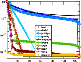
(a) Toolbox $n=128$ [20]

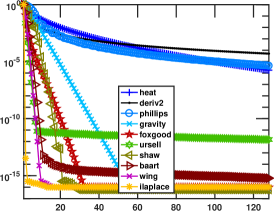
(b) Toolbox $n=256$ [20]

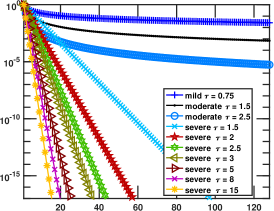
(c) Modeled decay rates

Figure 1. The singular value distribution for $n=128$ for noted examples from [20], normalized to $\sigma_{1}=1$ in Figure 1a. To show the independence of $n$, decay for $n=256$ for the same examples from [20] is also shown in Figure 1b. For each of the toolbox examples it is possible to compare with a simulated case for a specific decay rate by illustrating (4) for severe, moderate or mild decay choices of $\tau$, as appropriate, given in Figure 1c.

2.3. The Discrete Picard Condition and Noise Contamination

We now turn to the consideration of the noise in the coefficients $s_{i}=\mathbf{u}_{i}^{T}\mathbf{b}$ and the impact of this noise on the potential resolution in the solution, as also discussed in [21, §4.8.1]. First, we assume that the singular values satisfy a decay rate condition (4). We also assume that that the absolute values of the exact coefficients decay at least faster than the singular values

(9) $$(s^{2}_{i})_{\text{true}}\leq\sigma_{i}^{2(1+\nu)}\quad\text{for}\quad 0<\nu<1.$$

Then the discrete Picard condition is satisfied, [19], [21, Theorem 4.5.1].

When the noise in the data has common variance $\sigma^{2}$ we assume that there exists $\ell$ such that $E(s_{i}^{2})=\sigma^{2}$, for all $i>\ell$. Equivalently, we say that the coefficients are noise dominated for $i>\ell$. If this does not occur, then either the noise is insignificant, $\sigma^{2}<\sigma_{i}^{2}$ for all $i$, or totally dominates the solution $\sigma^{2}>1$, and these two cases are not of interest. Thus we can explicitly assume that there exists $\ell$ such that $\sigma_{\ell+1}<\sigma<\sigma_{\ell}$, and more precisely that

$$\sigma_{\ell+1}^{2}<\sigma^{1+\nu}_{\ell+1}<\sigma<\sigma^{1+\nu}_{\ell}<\sigma_{\ell},$$

where we use definition (4) as a continuous function of $i$ for a non integer index $\ell+\delta$.

Proposition 2.2.

Let $\sigma=\sigma_{\ell+\delta}^{1+\nu}$ for $0\leq\delta<1$ and $0<\nu<1$, then $E(s_{i}^{2})=\sigma^{2}$ for $i>\ell$ where

(10) $$\begin{array}[]{ll}\ell\approx\left\{\begin{array}[]{ll}\sigma^{-1/(\tau(1+\nu))}-\delta&\text{mild / moderate decay, }\\ (1-\delta)-\frac{\log\sigma}{(\nu+1)\log\tau}.&\text{severe decay.}\end{array}\right.\end{array}$$

Proof.

As in the proof of Proposition 2.1 we solve for $\ell$ dependent on the decay rate with respect to the upper bound in (10). This gives

$$\begin{array}[]{llll}\text{mild / moderate:}&(\ell+\delta)^{-\tau(1+\nu)}=\sigma\text{ implies }\ell=\sigma^{-1/(\tau(1+\nu))}-\delta,\\ \text{severe :}&\tau^{(1-(\ell+\delta))(1+\nu)}=\sigma\text{ implies }\ell=(1-\delta)-\frac{\log\sigma}{(\nu+1)\log\tau}.\end{array}$$

∎

Estimates using $\delta=\nu=0.5$ are indicated in Table 2 showing that the number of terms is relatively small even for moderate decay of the singular values for acceptable noise estimates $\sigma$. Contrasting with Table 1 we see that the number of coefficients that can be distinguished from the noise is generally less than the numerical rank of the problem for relevant noise levels and machine precision. This limits the number of the terms of the TSVD to use. In particular, suppose that $\alpha$ has to be found to filter the dominant noise terms with index $i\geq\ell$, then coefficients with $i\gg\ell$ will be further damped because the filter factors given in (2) decrease as a function of $i$. These terms then become insignificant in terms of the expansion for the solution.

Table 2. For different noise levels $\sigma$ the size of $\ell$ for given $\tau$ and with $\delta=\nu=0.5$. Entries calculated with rounding using (10).

$\tau$	$1.25$	$1.50$	$1.75$	$2.00$	$2.50$	$3.00$	$4.00$	$5.00$	$6.00$
$\sigma$	Moderate decay
$1\mathrm{e}{-1}$	$3$	$2$	$2$	$2$	$1$	$1$	$1$	$1$	1
${1\mathrm{e}{-2}}$	$11$	$7$	$5$	$4$	$3$	$2$	$2$	$1$	$1$
$1\mathrm{e}{-4}$	$135$	$59$	$33$	$21$	$11$	$7$	$4$	$3$	$2$
$1\mathrm{e}{-8}$	$18478$	$3593$	$1115$	$464$	$135$	$59$	$21$	$11$	$7$
$\sigma$	Severe decay
$1\mathrm{e}{-1}$	$7$	$4$	$3$	$3$	$2$	$2$	$2$	$1$	$1$
$1\mathrm{e}{-2}$	$14$	$8$	$6$	$5$	$4$	$3$	$3$	$2$	$2$
$1\mathrm{e}{-4}$	$28$	$16$	$11$	$9$	$7$	$6$	$5$	$4$	$4$
$1\mathrm{e}{-8}$	$56$	$31$	$22$	$18$	$14$	$12$	$9$	$8$	$7$

2.4. Regularization Parameter Estimation

We deduce from Tables 1 and 2 that the number of terms of the TSVD used for the solution of the regularized problem may strongly influence the choice for $\alpha$. Specifically the number of terms $k$ of the TSVD to use should be less than the numerical rank, $k<r$, and is dependent on the noise level in the data. We are interested in investigating the choice of $\alpha$ when obtained using the UPRE, but for comparison we also give the GCV function needed for the simulations, and note again that bounds on $\alpha$ dependent on $k$ have already been provided in [9]. The GCV and UPRE methods are derived without the use of the SVD, [11] and [41], resp., but it is convenient for the analysis to express both methods in terms of the SVD. Ignoring constant terms in the UPRE that do not impact the location of the minimum, introducing $\phi_{i}(\alpha)=1-\gamma_{i}(\alpha)=\alpha^{2}/(\sigma_{i}^{2}+\alpha^{2})$, and noting $\gamma_{i}(\alpha)=0$, for $i>k$, these are given by

(11) $$U_{k}(\alpha) = \sum_{i=1}^{k}(1-\gamma_{i}(\alpha))^{2}({\mathbf{u}}_{i}^{T}{\mathbf{b}})^{2}+2\sigma^{2}\sum_{i=1}^{k}\gamma_{i}(\alpha)=\sum_{i=1}^{k}\phi_{i}^{2}(\alpha)s_{i}^{2}+2\sigma^{2}\sum_{i=1}^{k}\gamma_{i}(\alpha),$$

(12) $$G_{k}(\alpha) = \frac{\sum_{i=1}^{m}(1-\gamma_{i}(\alpha))^{2}({\mathbf{u}}_{i}^{T}{\mathbf{b}})^{2}}{\left(\sum_{i=1}^{m}(1-\gamma_{i}(\alpha))\right)^{2}}=\frac{\sum_{i=1}^{k}\phi^{2}_{i}(\alpha)s_{i}^{2}+\sum_{i=k+1}^{m}s_{i}^{2}}{\left((m-k)+\sum_{i=1}^{k}\phi_{i}(\alpha)\right)^{2}}.$$

Here the subscript $k\leq r$ indicates that these are the expressions obtained using the TSVD, see e.g. [31, Appendix B] for derivations of the UPRE and GCV functions for arbitrary pairs $(m,n)$. Replacing $k$ by $r$ gives the standard functions for the full SVD. Further, we do not need all terms of the SVD to calculate the numerator in (12). Using $\|\mathbf{b}\|_{2}^{2}=\|U^{T}\mathbf{b}\|_{2}^{2}$ we can use

$$\sum_{i=k+1}^{m}({\mathbf{u}}_{i}^{T}{\mathbf{b}})^{2} = \|\mathbf{b}\|_{2}^{2}-\sum_{i=1}^{k}({\mathbf{u}}_{i}^{T}{\mathbf{b}})^{2}=\|\mathbf{b}\|_{2}^{2}-\sum_{i=1}^{k}s_{i}^{2}.$$

To illustrate how $\alpha_{k}$ varies when found using these functions we illustrate an example of a problem that is only moderately ill-posed ($\tau\approx 1.5$), showing the results of calculating the UPRE and GCV functions for data with noise variance $\sigma^{2}\approx 1\mathrm{e}{-4}$ and $\sigma^{2}\approx 1\mathrm{e}{-2}$ for the problem deriv2. The data and solution ${\mathbf{x}}_{\text{true}}$ are initially normalized so that $\|{\mathbf{b}}_{\text{true}}\|_{2}=1$. Consistent with the decay rate assumptions the singular values are normalized by $\sigma_{1}$. This requires additional normalization of ${\mathbf{b}}_{\text{true}}$ by $\sigma_{1}$, so that eventually $\|{\mathbf{b}}_{\text{true}}\|_{2}=\sigma_{1}^{-1}$. Then noise contaminated data are generated as $\mathbf{b}={\mathbf{b}}_{\text{true}}+\bm{\eta}$ for $\bm{\eta}\sim\mathcal{N}(0,\sigma^{2}I)$, for noise level $\sigma$. In these examples, the optimal value $\alpha_{k}$ is obtained by first evaluating $f(\alpha)$, $f(\alpha)=U_{k}(\alpha)$ or $f(\alpha)=G_{k}(\alpha)$ as specified in (11) or (12), resp., at $\sigma_{i}$, $1\leq i\leq k$. This provides $\alpha_{\mathrm{est}}=\textnormal{arg}\min_{1\leq i\leq k}f(\sigma_{i})$. This estimate of the minimum is used as the initial value for minimizing $f(\alpha)$ using Matlab fminbnd within the interval $[.01\alpha_{\mathrm{est}},100\alpha_{\mathrm{est}}]$. While this choice of lower and upper bounds on $\alpha_{k}$ is somewhat arbitrary, it is similar to the approach used in [20] for minimizing the UPRE and GCV functions, and is chosen to assure that values for $\alpha_{k}$ outside the interval $[\sigma_{k},\sigma_{1}]$ are possible when either $\alpha_{\mathrm{est}}=\sigma_{k}$ or $\sigma_{1}$. We pick this specific example in Figure 2 to highlight the discussion as applied to a problem which is not severely ill-posed. We also give the same information in Figure 3 for the severely ill-posed problem gravity ($\tau\approx 1.5$), see Figure 1a. To gain further insight the Picard plot, plots of $\sigma_{i}$, $|\mathbf{u}_{i}^{T}\mathbf{b}|$ and the ratio $|\mathbf{u}_{i}^{T}\mathbf{b}|/\sigma_{i}$, is given in each case in Figures 2b and 2d for deriv2 and in Figures 3b and 3d for gravity. The solutions are contaminated by noise very quickly for small $k$, corresponding to fast convergence of $\{\alpha_{k}\}$ with $k$.

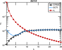
(a) $\alpha_{k}$ convergence. $\sigma^{2}\approx 1\mathrm{e}{-4}$.

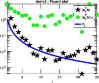
(b) Picard Plot. $\sigma^{2}\approx 1\mathrm{e}{-4}$.

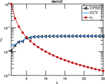
(c) $\alpha_{k}$ convergence. $\sigma^{2}\approx 1\mathrm{e}{-2}$.

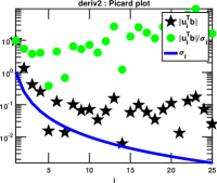
(d) Picard Plot. $\sigma^{2}\approx 1\mathrm{e}{-2}$.

Figure 2. Example deriv2 from [20] showing the convergence of $\{\alpha_{k}\}$ for UPRE and GCV functions for TSVD sizes of $1:25$ as compared to the decay of the singular values, for the original problem of size $128$ and the associated Picard plot for the data. In Figures 2a-2b, and Figures 2c-2d, the noise variances are $\sigma^{2}\approx 1\mathrm{e}{-4}$ and $\sigma^{2}\approx 1\mathrm{e}{-2}$, respectively. The converged relative errors in each case are $.273$ and $.381$ for the two noise variances $\sigma^{2}\approx 1\mathrm{e}{-4}$ and $\sigma^{2}\approx 1\mathrm{e}{-2}$, respectively.

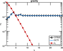
(a) $\alpha_{k}$ convergence. $\sigma^{2}\approx 1\mathrm{e}{-4}$.

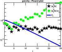
(b) Picard Plot. $\sigma^{2}\approx 1\mathrm{e}{-4}$.

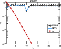
(c) $\alpha_{k}$ convergence. $\sigma^{2}\approx 1\mathrm{e}{-2}$.

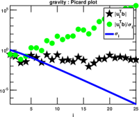
(d) Picard Plot. $\sigma^{2}\approx 1\mathrm{e}{-2}$.

Figure 3. Example gravity from [20] showing the convergence of $\{\alpha_{k}\}$ for UPRE and GCV functions for TSVD sizes of $1:25$ as compared to the decay of the singular values, for the original problem of size $128$ and the associated Picard plot for the data. In Figures 3a-3b, and Figures 3c-3d, the noise variances are $\sigma^{2}\approx 1\mathrm{e}{-4}$ and $\sigma^{2}\approx 1\mathrm{e}{-2}$, respectively. The converged relative errors for noise variance $\sigma^{2}\approx 1\mathrm{e}{-4}$ are $.644$ and $.655$ for UPRE and GCV respectively. For noise variance $\sigma^{2}\approx 1\mathrm{e}{-2}$, these errors are $.787$ and $1.143$, respectively.

Obtaining one-dimensional results, as shown in Figures 2-3, is trivial but motivates the theoretical study of convergence in Section 3, and then the application of that theory to standard two-dimensional problems in Section 4.

3. Theoretical Results

We aim to find effective practical bounds on the regularization parameter $\alpha$ when found using the UPRE function. Observe first that we would not expect the regularization parameter to be larger than $\sigma_{1}$, otherwise all filter factors are less than $1/2$. Indeed imposing $\alpha=\sigma_{1}$ would lead to over smoothed solutions, and all of the dominant singular value components (the components without noise contamination) would be represented in the solution with filtering e.g [22, Sections 4.4, 4.7]. In particular, the norm of the covariance matrix for the truncated filtered Tikhonov solution, the a posteriori covariance of the solution, is approximately bounded by $\sigma^{2}/(4\alpha^{2})$ which suggests smooth solutions for large $\alpha$. In contrast, the approximate bound for the a posteriori covariance when using the TSVD with $k$ terms without filtering is given by $\sigma^{2}/\sigma_{k}^{2}$ [22, Sections 4.4.2, 4.4]. Thus the filtered TSVD solution will be smoother than the TSVD solution when $\alpha>\sigma_{k}$: increasing $\alpha$ reduces the covariance but provides more smoothing. Practically it is reasonable to impose the upper bound $\alpha_{\mathrm{max}}\leq\sigma_{1}=1$ for $\alpha$. To limit the noise that can enter the solution it is also desirable to find the lower bound $\alpha_{\mathrm{min}}$. Solutions obtained for $\alpha\in[\alpha_{\mathrm{min}},\alpha_{\mathrm{max}}]$, dependent on the spectrum of $A$, should be sufficiently filtered but retain relatively unfiltered dominant components of the solution. We proceed to determine $\alpha_{\mathrm{min}}$ and to give a convergence analysis for $\alpha_{k}$ as the number of terms in the TSVD is increased.

3.1. Convergence of $\{\alpha_{k}\}$ calculated using UPRE

Denote the UPRE function (11) for the rank $r$ problem by $U(\alpha)=U_{r}(\alpha)$ and the optimal $\alpha$ for the filtered TSVD solution with $k$ components on the given interval as

(13) $$\alpha_{k}=\mathrm{argmin}_{\alpha\in[\alpha_{\mathrm{min}},\alpha_{\mathrm{max}}]}\,U_{k}(\alpha).$$

Ideally it would be helpful to find an interval $[\alpha_{\mathrm{min}},\alpha_{\mathrm{max}}]$ in which $U_{k}(\alpha)$ is strongly convex, but we have not been able to show this in general. Instead, in the following we show that a useful estimate of $\alpha_{\mathrm{min}}$ can be found.

For ease of notation within proofs we use $\phi_{i}$ and $\gamma_{i}$ to indicate $\phi_{i}(\alpha)$ and $\gamma_{i}(\alpha)$, respectively, and denote differentiation of a function $f(\alpha)$ with respect to $\alpha$ as $f^{\prime}$.

Proposition 3.1.

The following equalities are required for the future discussion.

(14) $$\frac{\partial U_{k}}{\partial\alpha} = \frac{4}{\alpha}\left(\sum_{i=1}^{k}s_{i}^{2}\phi^{2}_{i}(\alpha)\gamma_{i}(\alpha)-{\sigma^{2}}\sum_{i=1}^{k}\phi_{i}(\alpha)\gamma_{i}(\alpha)\right),$$

(15) $$\frac{\partial^{2}U_{k}}{\partial\alpha^{2}} = -\frac{1}{\alpha}\frac{\partial U_{k}}{\partial\alpha}+\frac{8}{\alpha^{2}}\left(\sum_{i=1}^{k}s_{i}^{2}\phi^{2}_{i}(\alpha)\gamma_{i}(\alpha)(2\gamma_{i}(\alpha)-\phi_{i}(\alpha))-\right.$$

$$\left.\sigma^{2}\sum_{i=1}^{k}\phi_{i}(\alpha)\gamma_{i}(\alpha)(\gamma_{i}(\alpha)-\phi_{i}(\alpha))\right).$$

Proof.

We use

$$\gamma_{i}^{\prime}=-\frac{2\alpha\sigma_{i}^{2}}{(\sigma_{i}^{2}+\alpha^{2})^{2}}=-\frac{2}{\alpha}\phi_{i}\gamma_{i}=-\phi_{i}^{\prime}<0.$$

Directly differentiating $U_{k}(\alpha)$ gives (14)

$$U^{\prime}_{k} = \sum_{i=1}^{k}s_{i}^{2}2\phi_{i}\phi_{i}^{\prime}+2\sigma^{2}\sum_{i=1}^{k}\gamma_{i}^{\prime}=\frac{4}{\alpha}\left(\sum_{i=1}^{k}s_{i}^{2}\phi^{2}_{i}\gamma_{i}-\sigma^{2}\sum_{i=1}^{k}\gamma_{i}\phi_{i}\right).$$

Likewise for the second derivative

(16) $$U^{\prime\prime}_{k} = -\frac{1}{\alpha}U^{\prime}_{k}+\frac{4}{\alpha}\left(\sum_{i=1}^{k}s_{i}^{2}(2\phi_{i}\phi_{i}^{\prime}\gamma_{i}+\phi^{2}_{i}\gamma_{i}^{\prime})-\sigma^{2}\sum_{i=1}^{k}(\phi_{i}^{\prime}\gamma_{i}+\phi_{i}\gamma_{i}^{\prime})\right),$$

giving (15) after substitution for the derivatives. ∎

Proposition 3.2.

Suppose that $0<\bar{\alpha}<{\sigma_{k}}/{\sqrt{2}}$ is a stationary point for $U_{k}(\alpha)$, for any $1\leq k\leq r$. Then $\bar{\alpha}$ is a unique minimum for $U_{k}({\alpha})$ on the interval $0<\bar{\alpha}<{\sigma_{k}}/{\sqrt{2}}$.

Proof.

Removing the first term from (16), identically zero at $\alpha=\bar{\alpha}$ by assumption that $\bar{\alpha}$ is a stationary point, gives

$$\frac{\partial^{2}U_{k}}{\partial\alpha^{2}}(\bar{\alpha}) = \frac{8}{\bar{\alpha}^{2}}\left(\sum_{i=1}^{k}s_{i}^{2}\phi^{2}_{i}(\bar{\alpha})\gamma_{i}(\bar{\alpha})(2\gamma_{i}(\bar{\alpha})-\phi_{i}(\bar{\alpha}))-\sigma^{2}\sum_{i=1}^{k}\phi_{i}(\bar{\alpha})\gamma_{i}(\bar{\alpha})(\gamma_{i}(\bar{\alpha})-\phi_{i}(\bar{\alpha}))\right)$$

$$= \frac{8}{\bar{\alpha}^{2}}\left(\sum_{i=1}^{k}s_{i}^{2}\phi^{2}_{i}(\bar{\alpha})\gamma_{i}(\bar{\alpha})(2-3\phi_{i}(\bar{\alpha}))-\sigma^{2}\sum_{i=1}^{k}\phi_{i}(\bar{\alpha})\gamma_{i}(\bar{\alpha})(1-2\phi_{i}(\bar{\alpha}))\right).$$

Now we substitute for $\sum_{i=1}^{k}s_{i}^{2}\phi^{2}_{i}(\bar{\alpha})\gamma_{i}(\bar{\alpha})=\sigma^{2}\sum_{i=1}^{k}\gamma_{i}(\bar{\alpha})\phi_{i}(\bar{\alpha})$ using (14) at $\bar{\alpha}$ and note all terms are positive for $1-3\phi_{i}(\bar{\alpha})>0$, $i=1:k$. But $\phi_{i}$ is increasing with $i$ due to the ordering of the $\sigma_{i}$. Thus $1-3\phi_{i}(\bar{\alpha})\geq 1-3\phi_{k}(\bar{\alpha})>0$ for $\bar{\alpha}<\sigma_{k}/\sqrt{2}$ and $U_{k}^{\prime\prime}(\bar{\alpha})>0$. This result is true for any stationary point $\bar{\alpha}$ on the interval. Hence $U_{k}(\bar{\alpha})$ is a minimum for $U_{k}(\alpha)$ and it is only possible to have a maximum at $\alpha=0$, the end point of the given interval, but the end point is explicitly excluded from consideration. There are therefore no other stationary points within the interval and the minimum is unique. ∎

Remark 3.1.

Although a minimum must exist in $[0,\sigma_{k}/\sqrt{2}]$ because $U_{k}(\alpha)$ is a continuous function on a compact set, this result does not show that a minimum exists in $(0,\sigma_{k}/\sqrt{2})$ .

The next steps in the analysis rely on the following Assumptions 1-2 about the model and the data.

Assumption 1 (Decay Rate, [21, 23]).

The measured coefficients decay according to $s^{2}_{i}=\sigma_{i}^{2(1+\nu)}>\sigma^{2}$ for $0<\nu<1$, $1\leq i\leq\ell$, i.e. the dominant measured coefficients follow the decay rate of the exact coefficients.

Assumption 2 (Noise in Coefficients).

There exists $\ell$ such that $E(s_{i}^{2})=\sigma^{2}$ for all $i>\ell$, i.e. that the coefficients $s_{i}$ are noise dominated for $i>\ell$. Moreover, when $i\leq\ell$ we assume that $E(s_{i}^{2})\approx s_{i}^{2}$, so that the larger coefficients are effectively deterministic.

These assumptions have also been used in [21] for understanding how decay rates impact the convergence of iterative methods. We also recall that we use the non-restrictive normalization $\sigma_{1}=1$ and use the notation $E(a)$ for the expectation of scalar deterministic $a$.

For the remaining results we distinguish between the terms in the UPRE function that are, and are not, contaminated by noise.

Proposition 3.3.

Suppose Assumption 2 holds, then for $r>k+1>\ell$ there is a an upper bound on $E(U_{k}^{\prime})$ independent of $\alpha$:

(17) $$E(\frac{\partial U_{r}}{\partial\alpha})<\dots<E(\frac{\partial U_{k+1}}{\partial\alpha}) < E(\frac{\partial U_{k}}{\partial\alpha})<\frac{\partial U_{\ell}}{\partial\alpha}\,\,\forall\,\,\alpha.$$

The lower bound for $E(U_{k}^{\prime\prime})$ holds for a fixed lower bound on $\alpha$

(18) $$E(\frac{\partial^{2}U_{r}}{\partial\alpha^{2}})>\dots>E(\frac{\partial^{2}U_{k+1}}{\partial\alpha^{2}}) > E(\frac{\partial^{2}U_{k}}{\partial\alpha^{2}})>\frac{\partial^{2}U_{\ell}}{\partial\alpha^{2}}\text{ if }\alpha>\frac{\sigma_{\ell+1}}{\sqrt{5}},$$

whereas the upper bound depends also on an upper bound on $\alpha$ that decreases with increasing $k$

(19) $$E(\frac{\partial^{2}U_{k+1}}{\partial\alpha^{2}}) < E(\frac{\partial^{2}U_{k}}{\partial\alpha^{2}})\,\,\text{if }\,\,\alpha<\frac{\sigma_{k+1}}{\sqrt{5}}.$$

Proof.

We note that the expectation operator is linear and when $a$ is not a random variable $E(a)=a$. Applying these properties first to (14) yields

$$E(U^{\prime}_{k}) = E\left(U^{\prime}_{\ell}+\frac{4}{\alpha}\sum_{i=\ell+1}^{k}\phi_{i}\gamma_{i}(s_{i}^{2}\phi_{i}-\sigma^{2})\right)$$

$$\approx U^{\prime}_{\ell}+\frac{4\sigma^{2}}{\alpha}\sum_{i=\ell+1}^{k}\phi_{i}\gamma_{i}(\phi_{i}-1)<U^{\prime}_{\ell},$$

where from line one to two we use linearity, and, by Assumption 2, $E(U^{\prime}_{\ell})=U^{\prime}_{\ell}$ and $E(s_{i}^{2})=\sigma^{2}$ for $i>\ell$. In particular, in expectation each term for $i>\ell$ is negative and recursively both inequalities in (17) apply. Applying the expectation operator now to (15) gives

$$E(U^{\prime\prime}_{k}) \approx \frac{\partial^{2}U^{\prime\prime}_{\ell}}{\partial\alpha^{2}}+\frac{4\sigma^{2}}{\alpha^{2}}\left(\sum_{i=\ell+1}^{k}\phi_{i}\gamma_{i}(1-\phi_{i})+2\left(\phi_{i}^{2}\gamma_{i}(2\gamma_{i}-\phi_{i})-\phi_{i}\gamma_{i}(\gamma_{i}-\phi_{i})\right)\right)$$

$$= U^{\prime\prime}_{\ell}+\frac{4\sigma^{2}}{\alpha^{2}}\left(\sum_{i=\ell+1}^{k}\phi_{i}\gamma_{i}\left(1-\phi_{i}+2\left(\phi_{i}(2\gamma_{i}-\phi_{i})-(\gamma_{i}-\phi_{i})\right)\right)\right)$$

$$= U^{\prime\prime}_{\ell}+\frac{4\sigma^{2}}{\alpha^{2}}\left(\sum_{i=\ell+1}^{k}\phi_{i}\gamma_{i}\left(1-\phi_{i}+2\left(\phi_{i}(2-3\phi_{i})-(1-2\phi_{i})\right)\right)\right)$$

$$= U^{\prime\prime}_{\ell}+\frac{4\sigma^{2}}{\alpha^{2}}\left(\sum_{i=\ell+1}^{k}\phi_{i}\gamma_{i}\left(-6\phi^{2}_{i}+7\phi_{i}-1\right)\right).$$

The sign of the second term depends on the sign of $-6\phi^{2}_{i}+7\phi_{i}-1$ which is increasing from $-1$ as a function of $\phi\leq 1$. Hence

$$-6\phi^{2}_{i}+7\phi_{i}-1\left\{\begin{array}[]{llcl}\geq-6\phi^{2}_{\ell+1}+7\phi_{\ell+1}-1&=\frac{\sigma_{\ell+1}^{2}(5\alpha^{2}-\sigma_{\ell+1}^{2})}{(\alpha^{2}+\sigma_{\ell+1}^{2})^{2}}&>0&\text{ if }\alpha>\frac{\sigma_{\ell+1}}{\sqrt{5}}\\ \leq-6\phi^{2}_{k}+7\phi_{k}-1&=\frac{\sigma_{k}^{2}(5\alpha^{2}-\sigma_{k}^{2})}{(\alpha^{2}+\sigma_{k}^{2})^{2}}&<0&\text{ if }\alpha<\frac{\sigma_{k}}{\sqrt{5}}.\end{array}\right.$$

Again, in expectation, terms for $i>\ell$ are all positive when $\alpha\geq{\sigma_{\ell+1}}/{\sqrt{5}}$ and the nested inequalities in (18) apply. The requirement that the $i^{th}$ term is necessarily positive becomes more severe as $i$ increases, yielding the additional inequality with conditions on $\alpha$ given in (19). ∎

Corollary 3.1.

Suppose Assumption 2 holds, and that for $\alpha_{\ell}>{\sigma_{\ell+1}}/{\sqrt{5}}$, $U_{\ell}(\alpha_{\ell})$ is a minimum for $U_{\ell}(\alpha)$. Then for $\ell<k\leq r$, $U_{k}(\alpha)$ is convex and decreasing at $\alpha_{\ell}$,

$$E(\frac{\partial U_{k}(\alpha_{\ell})}{\partial\alpha})<0\quad\text{and}\quad E(\frac{\partial^{2}U_{k}(\alpha_{\ell})}{\partial\alpha^{2}})>0.$$

Proof.

If $U_{\ell}(\alpha_{\ell})$ is a minimum, then $U^{\prime}_{\ell}(\alpha_{\ell})=0$ and $U^{\prime\prime}_{\ell}(\alpha_{\ell})>0$ and the inequalities follow immediately from (17) and (18). ∎

Corollary 3.2.

Suppose Assumption 2 holds. If a stationary point $\alpha_{r}<\sigma_{r}/\sqrt{5}$ exists there are no stationary points of $U_{k}(\alpha)$ for $\alpha\in(\sigma_{r}/\sqrt{5},\sigma_{k}/\sqrt{2})$.

Proof.

Suppose that $\alpha_{r}\in[0,\sigma_{r}/\sqrt{5})$. The existence of $\alpha_{r}$ in this interval does not contradict Proposition 3.2 since $\sigma_{r}/\sqrt{5}<\sigma_{r}/\sqrt{2}$. By assumption, $U^{\prime}_{r}(\alpha_{r})=0$ and $U^{\prime\prime}_{r}(\alpha_{r})>0$. Thus by (17) and (19) $U^{\prime}_{k}(\alpha_{r})>0$ and $U^{\prime\prime}_{k}(\alpha_{r})>0$, and $U_{k}(\alpha)$, $\ell\leq k\leq r-1$ is convex and increasing at $\alpha_{r}$. Therefore, by continuity, $U_{k}(\alpha)$ cannot reach a minimum for $\alpha_{r}<\alpha_{k}<\sigma_{k}/\sqrt{2}$ without first passing through a stationary point which is a maximum. But by Proposition 3.2 there is no maximum of $U_{k}(\alpha)$ to the left of $\sigma_{k}/\sqrt{2}$ and thus there is also no minimum for $\alpha_{r}<\alpha<\sigma_{k}/\sqrt{2}$. In particular $U_{k}(\alpha)$ has no stationary point for $\sigma_{r}/\sqrt{5}\leq\alpha\leq\sigma_{k}/\sqrt{2}$. ∎

Remark 3.2.

We have shown through Corollary 3.2 that if $U_{r}(\alpha_{r})$ is a minimum for $U_{r}(\alpha)$ and $\alpha_{r}<\sigma_{r}/\sqrt{5}$ then $U_{k}(\alpha_{k})$ can only be a minimum for $U_{k}(\alpha)$ if either $\alpha_{k}\leq\alpha_{r}\leq\sigma_{r}/\sqrt{5}$ or $\alpha_{k}>\sigma_{k}/\sqrt{2}$, i.e. we may require $\alpha_{k}>\sigma_{k}/\sqrt{2}$ under the assumption that we seek $\alpha_{r}>\sigma_{r}$. This applies for all $k$ with $1\leq\ell\leq k\leq r-1$.

Although this result does provide a refined lower bound for $\alpha_{k}$, it is dependent on $k$ and decreasing with $k$, which is not helpful when $k$ gets large, as needed for finding $\alpha_{r}$, i.e. this bound would suggest that $\alpha_{r}$ needs to be found using the pessimistic lower bound $\sigma_{r}/\sqrt{2}$. We investigate now whether these lower bounds on $\alpha$ are indeed realistic by looking for bounds on the UPRE functions $U_{k}(\alpha)$.

Proposition 3.4.

Suppose Assumptions 1 and 2 hold, then lower and upper bounds on $U_{k}(\alpha)$ and its derivatives are given by $\mathcal{L}_{k}(\alpha)$ and $\mathcal{U}_{k}(\alpha)$ and their derivatives, respectively, where

(21) $$0<\mathcal{L}_{k}(\alpha)=G(\alpha)+F_{k}(\alpha) <E(U_{k}(\alpha))<H(\alpha)+F_{k}(\alpha)=\mathcal{U}_{k}(\alpha)$$

(22) $$\mathcal{L}_{k}^{\prime}(\alpha)=G^{\prime}(\alpha)+F^{\prime}_{k}(\alpha) <E(U^{\prime}_{k}(\alpha))<H^{\prime}(\alpha)+F^{\prime}_{k}(\alpha)=\mathcal{U}_{k}^{\prime}(\alpha),$$

(23) $$\mathcal{L}_{k}^{\prime\prime}(\alpha)=G^{\prime\prime}(\alpha)+F^{\prime\prime}_{k}(\alpha) <E(U^{\prime\prime}_{k}(\alpha))<H^{\prime\prime}(\alpha)+F^{\prime\prime}_{k}(\alpha)=\mathcal{U}_{k}^{\prime\prime}(\alpha),\text{ for }\alpha\leq\sigma_{\ell}\text{ but }$$

$$\mathcal{U}_{k}^{\prime\prime}(\alpha)=H^{\prime\prime}(\alpha)+F^{\prime\prime}_{k}(\alpha) <E(U^{\prime\prime}_{k}(\alpha))<G^{\prime\prime}(\alpha)+F^{\prime\prime}_{k}(\alpha)=\mathcal{L}_{k}^{\prime\prime}(\alpha),\text{ for }\alpha>1.$$

Here $G(\alpha)$ and $H(\alpha)$ are independent of $k$, while $F_{k}(\alpha)$ very clearly depends on the $k$ terms in the sums as given by

(24) $$G(\alpha) = \alpha^{4}\sum_{i=1}^{\ell}\gamma^{2}_{i},\,\,H(\alpha)=\alpha^{2}\sum_{i=1}^{\ell}\phi_{i}\gamma_{i},\,\text{ and }$$

(25) $$F_{k}(\alpha) = \sigma^{2}\left((k-\ell)+2\sum_{i=1}^{\ell}\gamma_{i}+\sum_{i=\ell+1}^{k}\gamma_{i}^{2}\right).$$

Proof.

By (9) due to Assumption 1 for $i\leq\ell$

(26) $$\sigma_{i}^{4}<\sigma_{i}^{2(1+\nu)}=s_{i}^{2}<\sigma_{i}^{2}.$$

Thus

(27) $$\alpha^{4}\gamma_{i}^{2}=\sigma_{i}^{4}\phi_{i}^{2}<\phi_{i}^{2}(\alpha)s_{i}^{2}<\sigma_{i}^{2}\phi_{i}^{2}=\alpha^{2}\phi_{i}\gamma_{i}.$$

Now from (11)

$$E(U_{k}(\alpha)) = \sum_{i=1}^{\ell}\phi_{i}^{2}s_{i}^{2}+\sigma^{2}(2\sum_{i=1}^{k}\gamma_{i}(\alpha)+\sum_{i=\ell+1}^{k}\phi_{i}^{2})=\sum_{i=1}^{\ell}\phi_{i}^{2}s_{i}^{2}+F_{k}(\alpha),$$

may be bounded using (26). This yields immediately (21) with the noted definitions for $G$, $H$ and $F_{k}$, as given in (24)-(25).

To show (22) introduce $D_{i}(\alpha)>0$, $i=1$, $2$, given by

$$D_{1}(\alpha) = E(U_{k}(\alpha))-(G(\alpha)+F_{k}(\alpha))=\sum_{i=1}^{\ell}(\phi_{i}^{2}s_{i}^{2}-\alpha^{4}\gamma_{i}^{2})$$

$$D_{2}(\alpha) = (H(\alpha)+F_{k}(\alpha))-E(U_{k}(\alpha))=\sum_{i=1}^{\ell}(\alpha^{2}\phi_{i}\gamma_{i}-\phi_{i}^{2}s_{i}^{2}).$$

Then $D_{i}$ are independent of $k$ and

$$D^{\prime}_{1}(\alpha) = \sum_{i=1}^{\ell}\left(\frac{2}{\alpha}(2\phi^{2}_{i}\gamma_{i}s_{i}^{2}+2\alpha^{4}\gamma^{2}_{i}\phi_{i})-4\alpha^{3}\gamma_{i}^{2}\right)=\frac{4}{\alpha}\sum_{i=1}^{\ell}(\phi^{2}_{i}\gamma_{i}s_{i}^{2}-\alpha^{4}\gamma^{3}_{i})\text{ and }$$

$$D^{\prime}_{2}(\alpha) = \sum_{i=1}^{\ell}(2\alpha\phi_{i}\gamma_{i}+\frac{2}{\alpha}(\alpha^{2}\phi_{i}\gamma_{i}(1-2\phi_{i})-2\phi_{i}^{2}\gamma_{i}s_{i}^{2}))=\frac{4}{\alpha}\sum_{i=1}^{\ell}(\alpha^{2}\phi_{i}\gamma_{i}^{2}-s_{i}^{2}\phi_{i}^{2}\gamma_{i}).$$

But now again applying Assumption 1 we have

(28) $$\alpha^{4}\gamma_{i}^{3}=\sigma_{i}^{4}\phi^{2}_{i}\gamma_{i}<{s^{2}_{i}}\phi^{2}_{i}\gamma_{i}<\sigma_{i}^{2}\phi^{2}_{i}\gamma_{i}=\alpha^{2}\phi_{i}\gamma_{i}^{2}.$$

Therefore $D_{i}^{\prime}(\alpha)>0$, $i=1$, $2$ and we immediately obtain (22).

The second derivative result follows similarly using

$$D^{\prime\prime}_{1}(\alpha) = \frac{12}{\alpha^{2}}\sum_{i=1}^{\ell}\gamma_{i}(1-2\phi_{i})(s_{i}^{2}\phi_{i}^{2}-\alpha^{4}\gamma_{i}^{2})>0$$

$$D^{\prime\prime}_{2}(\alpha) = \frac{12}{\alpha^{2}}\sum_{i=1}^{\ell}\phi_{i}\gamma_{i}(1-2\phi_{i})(\gamma_{i}\alpha^{2}-s_{i}^{2}\phi_{i})>0,$$

where in each case we apply (28) and note $1-2\phi_{i}\geq 0$, for $1\leq i\leq\ell$ and $\alpha\leq\sigma_{\ell}$. This then immediately gives the reverse inequalities for $\alpha>1$. ∎

From (24)-(25) we see that we may write $G$, $H$ and $F_{k}$ in terms of sums $S_{p}(i_{1},i_{2})=\sum_{i=i_{1}}^{i_{2}}\gamma^{p}_{i}$ for $p=1$ and $p=2$ by writing $\phi_{i}\gamma_{i}=\gamma_{i}-\gamma_{i}^{2}$. Hence

$$G(\alpha)=\alpha^{4}S_{2}(1,\ell),\,\,H(\alpha)=\alpha^{2}(S_{1}(1,\ell)-S_{2}(1,\ell))\quad\mathrm{and}$$

$$\,\,F_{k}(\alpha)=\sigma^{2}(k-\ell+2S_{1}(1,\ell)+S_{2}(\ell+1,k)).$$

Thus for $U_{\ell}(\alpha)$ we have the bounding functions by Proposition 3.3

$$\mathcal{L}_{\ell}(\alpha) = G(\alpha)+F_{\ell}(\alpha)=\alpha^{4}S_{2}+2\sigma^{2}S_{1}$$

$$\mathcal{U}_{\ell}(\alpha) = H(\alpha)+F_{\ell}(\alpha)=\alpha^{2}(S_{1}-S_{2})+2\sigma^{2}S_{1},$$

where the sums all range from $1$ to $\ell$. Moreover, also by Proposition 3.3, $\mathcal{L}_{\ell}^{\prime}(\alpha)<U_{\ell}(\alpha)<\mathcal{U}_{\ell}^{\prime}(\alpha)$ where

$$\mathcal{L}_{\ell}^{\prime}(\alpha) = 4\alpha^{3}S_{2}+\alpha^{4}S_{2}^{\prime}+2\sigma^{2}S^{\prime}_{1}=4\alpha^{3}(S_{2}+S_{3}-S_{2})+\frac{4\sigma^{2}}{\alpha}(S_{2}-S_{1})$$

$$= \frac{4}{\alpha}(\alpha^{4}S_{3}+\sigma^{2}(S_{2}-S_{1}))$$

$$\mathcal{U}_{\ell}^{\prime}(\alpha) = 2\alpha(S_{1}-S_{2})+\alpha^{2}(S_{1}^{\prime}-S_{2}^{\prime})+2\sigma^{2}S^{\prime}_{1}$$

$$= 2\alpha(S_{1}-S_{2})+2\alpha(S_{2}-S_{1}-2(S_{3}-S_{2}))+\frac{4}{\alpha}\sigma^{2}(S_{2}-S_{1})$$

$$= \frac{4}{\alpha}(\alpha^{2}(S_{2}-S_{3})+\sigma^{2}(S_{2}-S_{1})),$$

and we used $\gamma_{i}^{\prime}=-({2}/{\alpha})\gamma_{i}\phi_{i}=({2}/{\alpha})(\gamma_{i}^{2}-\gamma_{i})$ and $(\gamma_{i}^{2})^{\prime}=-({4}/{\alpha})\gamma^{2}_{i}\phi_{i}=({4}/{\alpha})(\gamma_{i}^{3}-\gamma_{i}^{2})$.

Proposition 3.5.

Suppose Assumption 1 holds, then necessarily $U_{\ell}^{\prime}(\alpha)<0$ for $\alpha^{2}<\sigma_{\ell+1}^{2}/(1-\sigma_{\ell+1}^{2})$. Hence $\alpha^{2}_{\ell}>\sigma^{2}_{\ell+1}/(1-\sigma^{2}_{\ell+1})$.

Proof.

If the upper bound has a negative slope, $\mathcal{U}_{\ell}^{\prime}(\alpha)<0$ for some $\alpha$, then $U_{\ell}^{\prime}(\alpha)<0$ also. Immediately $\mathcal{U}_{\ell}^{\prime}(\alpha)<0$ for $\alpha^{2}(S_{2}-S_{3})+\sigma^{2}(S_{2}-S_{1})<0$, and for $U_{\ell}^{\prime}(\alpha)<0$ it is sufficient that for $1\leq i\leq\ell$

$$0 > \alpha^{2}(\gamma_{i}^{2}-\gamma_{i}^{3})+\sigma^{2}(\gamma_{i}^{2}-\gamma_{i})=\gamma_{i}(\alpha^{2}\gamma_{i}(1-\gamma_{i})+\sigma^{2}(\gamma_{i}-1))=\gamma_{i}\phi_{i}(\alpha^{2}\gamma_{i}-\sigma^{2}),$$

and we need $(\alpha^{2}\gamma_{i}-\sigma^{2})<0$, or $\alpha^{2}\sigma_{i}^{2}-\sigma^{2}(\alpha^{2}+\sigma_{i}^{2})<0$. Now, for $i\leq\ell$, $\sigma_{i}^{2}\geq\sigma_{\ell}^{2}>\sigma^{2}$ and we obtain $\alpha^{2}<\min({\sigma^{2}\sigma_{i}^{2}}/{(\sigma_{i}^{2}-\sigma^{2})})$ for all $1\leq i\leq\ell$. But $x^{2}/(x^{2}-a^{2})$ is decreasing with $x$ for $x^{2}>a^{2}$, hence we need $\alpha^{2}<\sigma^{2}/(1-\sigma^{2})$. For $\sigma_{\ell+1}^{2}<\sigma^{2}<\sigma_{\ell}^{2}$ and using $x^{2}/(1-x^{2})$, which is increasing with $x\in(0,1)$, we obtain $\alpha^{2}<\sigma_{\ell+1}^{2}/(1-\sigma_{\ell+1}^{2})$. Hence we must have $\alpha^{2}_{\ell}>\sigma^{2}_{\ell+1}/(1-\sigma^{2}_{\ell+1})$. ∎

We now extend the analysis to obtain a lower bound on $\alpha_{k}$ for all $k>\ell$.

Theorem 3.1.

Suppose Assumptions 1 and 2 hold, and that $U_{k}(\alpha_{k})$ is a minimum for $U_{k}(\alpha)$, then, for $k\geq\ell$, $\alpha_{k}>\alpha_{\ell}>\sigma_{\ell+1}/\sqrt{1-\sigma_{\ell+1}^{2}}=\alpha_{\mathrm{min}}$.

Proof.

First suppose the contrary and that $\alpha_{k}\leq\sigma_{\ell+1}/\sqrt{1-\sigma_{\ell+1}^{2}}$. Then $U_{k}^{\prime}(\alpha_{k})=0$ and by (17) $U^{\prime}_{\ell}(\alpha_{k})>0$. But by Proposition 3.5 $U^{\prime}_{\ell}(\alpha)<0$ for $\alpha\leq\sigma_{\ell+1}/\sqrt{1-\sigma_{\ell+1}^{2}}$ and we have a contradiction yielding $\alpha_{k}>\sigma_{\ell+1}/\sqrt{1-\sigma_{\ell+1}^{2}}=\alpha_{\mathrm{min}}$, $k\geq\ell$. It remains to determine whether it is possible to have $\sigma_{\ell+1}/\sqrt{1-\sigma_{\ell+1}^{2}}<\alpha_{k}<\alpha_{\ell}$ where $\alpha_{\ell}$ is the first minimum point of $U_{\ell}(\alpha)$ to the right of $\alpha_{\mathrm{min}}$. Again we proceed by contradiction and suppose that $\alpha_{k}\in[\alpha_{\mathrm{min}},\alpha_{\ell}]$ exists. Then we have the following:

1. By (17) $E(U_{k}^{\prime})(\alpha_{\ell})<U_{\ell}^{\prime}(\alpha_{\ell})=0$, and by (18), noting $\alpha>\sigma_{\ell+1}/\sqrt{5}$, $E(U^{\prime\prime}_{k})(\alpha_{\ell})>U^{\prime\prime}_{\ell}(\alpha_{\ell})>0$. Hence $U_{k}(\alpha)$ is convex and decreasing at $\alpha_{\ell}$.

2. At the minimum critical point $\alpha_{k}<\alpha_{\ell}$, $U_{k}^{\prime}(\alpha_{k})=0$. Thus there must also be a second critical point which is a maximum for some $\bar{\alpha}$ in the interval $\alpha_{k}<\bar{\alpha}<\alpha_{\ell}$, for which $U_{k}^{\prime}(\bar{\alpha})=0$ and $U_{k}^{\prime\prime}(\bar{\alpha})<0$.

3. At $\bar{\alpha}$ we then have by (17) that $U^{\prime}_{\ell}(\bar{\alpha})>0$. Hence $U_{\ell}(\alpha)$ is increasing at $\bar{\alpha}<\alpha_{\ell}$ but is decreasing at $\alpha_{\mathrm{min}}<\bar{\alpha}$, i. e. $U_{\ell}^{\prime}(\alpha)$ changes sign for some $\alpha$ in the interval $[\alpha_{\mathrm{min}},\bar{\alpha}]$. But by continuity then $U_{\ell}(\alpha)$ has at least one minimum on this interval. By assumption, however, $\alpha_{\ell}$ is the first minimum point of $U_{\ell}(\alpha)$ to the right of $\alpha_{\mathrm{min}}$ and we have arrived at a contradiction.

∎

We have now obtained a tight lower bound on $\alpha_{k}$

(29) $$\alpha_{\mathrm{min}}=\frac{\sigma_{\ell+1}}{\sqrt{1-\sigma^{2}_{\ell+1}}}<\alpha_{k},\quad\ell\leq k\leq r.$$

It remains to discuss the convergence of $\{\alpha_{k}\}$ to $\alpha_{k_{\mathrm{opt}}}$ with increasing $k$. We note that one approach would be to show that the $U_{k}(\alpha)$ are convex for $\alpha>\sigma_{\ell}$, but the sign result in (23) only immediately applies for $\alpha>1$, hence investigating the sign requires a more refined bound for each interval $\alpha\in[\sigma_{i},\sigma_{i-1}]$ for $i\leq\ell$. Instead we obtain the following result, which relies on the uniqueness of $\alpha_{k}$.

Theorem 3.2.

Suppose Assumptions 1 and 2 hold and that $\alpha_{k_{\mathrm{opt}}}$ and each $\alpha_{k}$, $k>\ell$ are unique within the given interval $\sigma_{\ell+1}/\sqrt{1-\sigma^{2}_{\ell+1}}<\alpha<1$. Then, the sequence $\{\alpha_{k}\}_{k>\ell}$ is on the average increasing with $\lim_{k\rightarrow r}E(\alpha_{k})=E(\alpha_{k_{\mathrm{opt}}})$ and $\{U_{k}(\alpha_{k})\}$ is increasing.

Proof.

It is immediate from (11) that $U_{k}(\alpha)\geq U_{\ell}(\alpha)$ for any $k>\ell$ and any $\alpha$, and that $U_{k+1}(\alpha)\geq U_{k}(\alpha)$. Thus the $\{U_{k}(\alpha)\}$ is an increasing set of functions with $k>\ell$. By (17) of Proposition 3.3 we also have $E(\frac{\partial U_{k+1}(\alpha)}{\partial\alpha})<E(\frac{\partial U_{k}(\alpha)}{\partial\alpha})<\frac{\partial U_{\ell}(\alpha)}{\partial\alpha}$, and $\{E(\frac{\partial U_{k}(\alpha)}{\partial\alpha})\}$ is a decreasing set of functions for $k>\ell$. In particular $E(\frac{\partial U_{k+1}(\alpha_{\ell})}{\partial\alpha})<E(\frac{\partial U_{k}(\alpha_{\ell})}{\partial\alpha})<0$. Moreover, by Corollary 3.1 and (18) of Proposition 3.3, when $\alpha_{\ell}>{\sigma_{\ell+1}}/{\sqrt{5}}$ the expected second derivatives at $\alpha_{\ell}$ are positive and increasing with $k$ so that the first derivative increases to $0$ more quickly for larger $k$. Thus, not only do we have $E(\alpha_{k})>\alpha_{\ell}>\alpha_{\mathrm{min}}$ for all $k$, we also have that $\{E(\alpha_{k})\}$ converges from below to $E(\alpha_{k_{\mathrm{opt}}})$. ∎

Corollary 3.3 (Faster Decay Rate of the Coefficients).

Suppose that the coefficients $s_{i}$ decay at the rate $s_{i}^{2}=\sigma_{i}^{2(\rho+\nu)}$ for integer $\rho>1$. Then the results of Theorems 3.1-3.2 still hold.

Proof.

This holds by modifying the inequality (9) for the faster decay rate yielding

$$K_{i}\sigma_{i}^{4}<\sigma_{i}^{2(\rho+\nu)}=s_{i}^{2}<\sigma_{i}^{2}K_{i},\quad K_{i}=\sigma_{i}^{2(\rho-1)}.$$

Thus the coefficients are bounded as in (27) but with scale factor $K_{i}$

$$\alpha^{4}\gamma_{i}^{2}K_{i}=\sigma_{i}^{4}\phi_{i}^{2}K_{i} < \phi_{i}^{2}(\alpha)s_{i}^{2}<K_{i}\sigma_{i}^{2}\phi_{i}^{2}=K_{i}\alpha^{2}\phi_{i}\gamma_{i}.$$

Using this relation all the results presented in Proposition 3.4 still hold with $H(\alpha)$ and $G(\alpha)$ replaced by

$$G_{\rho}(\alpha)=\alpha^{4}\sum_{i=1}^{\ell}K_{i}\gamma^{2}_{i},\quad\text{and}\quad H_{\rho}(\alpha)=\alpha^{2}\sum_{i=1}^{\ell}K_{i}\phi_{i}\gamma_{i}.$$

Then again redefining the summations $S_{p}$ to now depend on the coefficients with $K_{i}$, for $H_{\rho}$ and $G_{\rho}$, following Proposition 3.5 yields the condition

$$\gamma_{i}\phi_{i}(\alpha^{2}K_{i}\gamma_{i}-\sigma^{2})<0$$

for $U^{\prime}_{\ell}(\alpha)<0$. Continuing the argument as in the proof of Proposition 3.5 still yields the lower bound $\alpha_{\ell}^{2}>\sigma_{\ell+1}^{2}/(1-\sigma_{\ell+1}^{2})$. But this is all that is required for Theorems 3.1-3.2 and hence the results follow without modification. ∎

Remark 3.3.

This result shows that given a TSVD which sufficiently incorporates the dominant terms of the SVD expansion, including sufficient terms that are noise-contaminated, $\alpha_{k}$ will be an increasingly good approximation for $\alpha_{k_{\mathrm{opt}}}$. Moreover, including additional terms in the expansion will have limited impact on the solution, because $\alpha_{k_{\mathrm{opt}}}>\alpha_{\ell}$ and filter factor $\gamma_{i}(\alpha_{k_{\mathrm{opt}}})$ is decreasing with $i$. In particular, we are using $\gamma_{i}(\alpha_{k_{\mathrm{opt}}})<\gamma_{i}(\alpha_{\ell})<\gamma_{\ell+1}(\alpha_{\ell})<\gamma_{\ell+1}(\sigma_{\ell+1})=1/2$, for $i>\ell+1$ and $\alpha_{\ell}>\sigma_{\ell+1}$. These nested inequalities follow immediately because $\gamma(x,y)=y^{2}(y^{2}+x^{2})^{-1}$ is decreasing as a function of $x$ and increasing as a function of $y$.

Remark 3.4.

Although the main result of this paper effectively relies on an assumption that the UPRE functions have unique minima within the obtained bounds, $\alpha_{\mathrm{min}}<\alpha_{k}<1$, proving that the minima are indeed unique seems to require using the discrete summations occurring in $U_{k}(\alpha)$ as approximations to continuous integrals. This approach is very technical, not very general, being dependent on the decay rate parameter $\tau$, and serves only to tighten the lower bound for $\alpha$. We therefore chose not to present results along this direction, relying on the computational results that are supportive of the unique identification of a minimum within these realistic bounds.

Remark 3.5.

The results given depend on the assumption that summations with $s_{i}^{2}$ for terms with $i>\ell$ may be approximated in terms of the noise variance. For $r-\ell$ small relative to $r$, this assumption breaks down. As $r-\ell$ increases the assumptions become more reliable and less impacted by outlier data for $s_{i}^{2}$. Still the main convergence theorem holds only with respect to this analysis and we cannot expect that $\{\alpha_{k}\}$ will always converge monotonically to $\alpha_{k_{\mathrm{opt}}}$ in practice. With sufficient safeguarding, as noted in the algorithm presented in Section 4, it is reasonable to expect that $\alpha_{k_{\mathrm{opt}}}$ is quickly and accurately identified.

Remark 3.6 (Posterior Covariance).

We have shown $\{\alpha_{k}\}$ increases with $k$. Consequently, the approximate a posteriori covariance of the filtered TSVD solution $\sigma^{2}/(4\alpha^{2})$ decreases with $k$, to $\sigma^{2}/(4\alpha_{k_{\mathrm{opt}}}^{2})$. In trading-off the minimization of the risk by using the UPRE to find the optimal $\alpha$, the method naturally finds a solution which has increasing smoothness with increasing $k$. This limits the impact of the possibly non-smooth components of the solution corresponding to small singular values, most likely noise-contaminated, that would contaminate the unfiltered TSVD solution.

4. Practical Application

The convergence theory for $\{\alpha_{k}\}\rightarrow\alpha_{k_{\mathrm{opt}}}$ as $k\rightarrow k_{\mathrm{opt}}$ presented in Section 3 motivates the construction of an algorithm to automatically determine the optimal index $k_{\mathrm{opt}}$, defined as in Section 1 to be the optimal number of terms to use from the TSVD, and associated regularization parameter $\alpha_{k_{\mathrm{opt}}}$. The algorithm is presented and discussed in Section 4.1 and tested for $2D$ test problems using IR Tools [10] in Section 4.2. These results also corroborate the convergence theory presented in Section 3.

4.1. Algorithm

We propose an algorithm that works by iteratively minimizing (11) on the TSVD subspace of size $k\leq r$ until a set of convergence criteria are met. These convergence criteria rest on the observation that in general for sufficiently large $k$, the relative change, $c_{k}=|(\alpha_{k}-\alpha_{k+1})|/\alpha_{k}>0$, between successive parameter estimates, $\alpha_{k}$ and $\alpha_{k+1}$, decreases as $k$ increases towards $r$. If during the iterative procedure there exists a $k$ such that it is reasonably believed that $\alpha_{k}\approx\alpha_{i}$ for all $i>k$, the algorithm terminates, producing $k_{\mathrm{opt}}$ and $\alpha_{k_{\mathrm{opt}}}$. A pseudo-code implementation is given as Algorithm 1.

Input:  SVD or TSVD; data $\mathbf{b}$ and noise variance estimate $\sigma^{2}$; initial index $k_{0}$; maximum $k$, $k_{\text{max}}$; step size $\Delta_{k}$; relative tolerance $\delta$; window length $w$; optional estimate for $\ell$

Output:  Converged parameter $\alpha_{k_{\mathrm{opt}}}$; convergence index $k_{\mathrm{opt}}$; relative mean change $\hat{c}_{iw}$;

1

2$k\longleftarrow k_{0};\quad\hat{c}_{iw}\longleftarrow\text{inf}$

3 Initialize $\alpha_{\mathrm{min}}$ according to (29) using $\ell$ if provided, otherwise using $k$

4 $\alpha(0)\longleftarrow\textnormal{arg}\min_{\alpha}U_{k}(\alpha)$ over interval $[\alpha_{\mathrm{min}},1]$

5 while  $(\hat{c}_{iw}>\delta$ and $k<k_{\text{max}})$ or $(\alpha(i)=\alpha_{\mathrm{min}})$ do

6       $i\longleftarrow i+1;\quad k\longleftarrow k+\Delta_{k}$

7       If $\ell$ not provided, update $\alpha_{\mathrm{min}}$ according to (29) using $k$

8       $\alpha(i)\longleftarrow\textnormal{arg}\min_{\alpha}U_{k}(\alpha)$ over interval $[\alpha_{\mathrm{min}},1]$

9       $c(i)=(|\alpha(i)-\alpha(i-1)|)/\alpha(i)$

10       if $i\geq w$ then

11             $\hat{c}_{iw}\longleftarrow\textnormal{{mean}}(c(i),c(i-1),\dots,c(i-w+1))$

12            

13       end if

14      

15 end while

16

return $k=k_{\mathrm{opt}}$, $\alpha(i)=\alpha_{k_{\mathrm{opt}}}$, $\hat{c}_{iw}$

Algorithm 1 Truncated UPRE Parameter Estimation

Algorithm 1 takes as input a full or truncated SVD as well as a number of required and optional parameters which we now discuss. For large scale problems it is not necessary, and is even discouraged, to compute $\alpha_{k}$ for all $k\leq k_{\mathrm{opt}}$. For moderately or mildly ill-posed problems, and for problems with high signal to noise ratios in which the expected $k_{\mathrm{opt}}$ is likely to be large relative to the problem size, it is recommended to start the algorithm at some $k_{0}\neq 1$ and to increment $k$ by some $\Delta_{k}\neq 1$, yielding the sequence $\{k(i):k_{0},k_{0}+\Delta_{k},k_{0}+2\Delta_{k},\dots k_{0}+i\Delta_{k}\}$. The algorithm computes the sequence $\{\alpha_{k_{0}},\alpha_{k_{0}+\Delta_{k}},\alpha_{k_{0}+2\Delta_{k}},\alpha_{k_{0}+3\Delta_{k}},\dots\}$, each solving (13) for the given index, until either $k_{0}+i\Delta_{k}\geq k_{\text{max}}$ or until $\alpha_{k}$ has converged, where $k_{0}$, $\Delta_{k}$, and $k_{\text{max}}$ are provided by the user. For each $k_{0}+i\Delta_{k}$ the relative change in $\alpha$ is computed as $c_{i}=|\alpha_{k_{0}+i\Delta_{k}}-\alpha_{k_{0}+(i-1)\Delta_{k}}|/\alpha_{k_{0}+i\Delta_{k}}$. Noting again that $c_{i}$ is only in general decreasing for sufficiently large $i$, it is unwise to determine stopping criteria by directly thresholding on $c_{i}<\delta$, for some user provided tolerance $\delta$. It is observed that higher confidence in convergence can be achieved by requiring $\hat{c}_{iw}<\delta$ where $\hat{c}_{iw}$ is the mean of multiple $c_{i}$’s calculated over the window of size $w$, i.e. over $\{c_{i},c_{i+1},\dots,c_{i+w}\}$. This protects against the possibility of stopping the parameter search too early and prior to the stabilization of $\alpha_{k}$. This occurs when $c_{i}<\delta$, while at the same time $c_{j}\geq\delta$ for some $j>i$. Due to the impact of noise on calculating the parameter $\alpha_{k}$, if $k$ is not yet sufficiently large so that $\alpha_{k}$ has not stabilized then the relative changes between successive estimates of $\alpha_{k}$ may be either extremely small or large. Comparing multiple values of $c_{i}$ in the form of $\hat{c}_{iw}$ to $\delta$ enables a broader view of the convergence of $\alpha_{k}$, and the moving window average smooths out variation in $c_{i}$.

Remark 4.1 (Parameter $\Delta_{k}$).

The choice of $\Delta_{k}$ is influenced by the size of the problem and if known, an estimate for the expected number of terms to be used in the TSVD solution. While choosing $\Delta_{k}$ large has computational advantages due to a larger step size in the search for $k_{\mathrm{opt}}$, with $\Delta_{k}$ too large one risks the possibility of Algorithm 1 producing a value of $k_{\mathrm{opt}}$ larger than necessary. Solutions with $k_{\mathrm{opt}}$ larger than necessary more closely resemble the full UPRE regularized solution. For the problem sizes considered here $\Delta_{k}\in\{5,10,25\}$ all seemed to work well.

Remark 4.2 (Parameter $w$).

The choice of $w$ has a similar effect as $\Delta_{k}$. Choosing $w$ large will delay the termination criteria . Parameters $\Delta_{k}$ and $w$ interact in the sense that they together determine the set $\{c_{i},c_{i+1},\dots,c_{i+w}\}$ whose mean is compared to $\delta$ in determining convergence. The choice of $w$ determines how many values are being averaged, while $w$ and $\Delta_{k}$ determine the minimum and maximum $k$ of the moving window over which $\alpha_{k}$ is tested for convergence. Choosing $w\in\{5,10,25,50\}$ worked well for the problems considered here.

Remark 4.3 (Parameter $\delta$).

Algorithm 1 is sensitive to $\delta$ and we recommend choosing $\delta\in[1\mathrm{e}{-5},1\mathrm{e}{-3}]$. In our experiments $\delta>1\mathrm{e}{-3}$ terminated the algorithm prior to convergence resulting in over smoothed solutions due to an underestimate of $k_{\mathrm{opt}}$, while $\delta<1\mathrm{e}{-5}$ produced $k_{\mathrm{opt}}$ far greater than necessary.

To summarize, the required input to the proposed algorithm is a full or truncated SVD, a starting index $k_{0}$, a step size between successive estimates $\Delta_{k}$, an upper-bound $k_{\text{max}}$ dependent on the severity of the problem and the noise level, a tolerance $\delta$, and a width $w$ over which the moving average of relative changes in successive estimates of $\alpha$ is computed.

The results of Theorem 3.1 are incorporated into Algorithm 1 with the inclusion of an optional parameter $\ell$ specifying an estimate for the index at which noise dominates the coefficients. If a Picard plot is available $\ell$ can be estimated visually, otherwise an approach relying on Picard parameter estimates similar to that used by [34] and [24] can be used. If an estimate for $\ell$ is available, $\alpha_{\mathrm{min}}$ is calculated according to (29), and $\alpha_{k}$ is found using $\alpha_{\mathrm{min}}=\sigma_{\ell+1}/\sqrt{1-\sigma_{\ell+1}^{2}}$ and $\alpha_{\mathrm{max}}=1$ in (13). Otherwise, the bound $\sigma_{k+1}/\sqrt{1-\sigma_{k+1}^{2}}$ is used in (13). In either case if the lower bound is achieved then the theory indicates that noise has not yet dominated and the algorithm is allowed to continue. Thus, in the case where $k<k_{\text{max}}$, necessary conditions for the termination of Algorithm 1 are $\hat{c}_{iw}<\delta$ and $\alpha_{k}$ should be greater than the specified $\alpha_{\mathrm{min}}$.

4.2. Verification of the Algorithm and Theory

We now present the evaluation of Algorithm 1 on a 2D test problem using the IR Tools package described in [10]. We report the results applying a Gaussian blur to test problem Satellite of size $256\times 256$ using PRblur, with medium blur. We considered noise levels of $5\%$, $10\%$, and $25\%$, with $100$ noise instances generated for each noise level. The IR Tools function PRnoise was used to generate noise, where the noise level is defined as as $\|\mathbf{\eta}\|_{2}/\|\mathbf{b}\|$. A moving window of size $w=5$ in computing $\hat{c}_{iw}$ with relative tolerance of $\delta=1\mathrm{e}{-3}$ was found to work well for each noise level, but may need to be adapted to the severity of the ill-posedness of the problem. Recorded in each run are the converged $\alpha_{k_{\mathrm{opt}}}$, the size of the TSVD subspace $k_{\mathrm{opt}}$ to be used, and the relative reconstruction error (RRE). RRE is defined as $\|x_{\text{true}}-x_{k_{\mathrm{opt}}}\|_{2}/\|x_{\text{true}}\|_{2}$ where $x_{k_{\mathrm{opt}}}$ is the filtered, $k_{\mathrm{opt}}$-truncated TSVD solution obtained by using $\alpha_{k_{\mathrm{opt}}}$ as the regularization parameter.

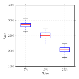
Figure 4. Box plots showing the index $k_{\mathrm{opt}}$ produced by Algorithm 1 for problem Satellite computed from $100$ runs for noise levels $5\%$, $10\%$, and $25\%$. The number of terms $k$ in the TSVD that provide useful information decreases as the noise level increases.

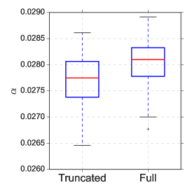
(a) Noise level $=5\%$

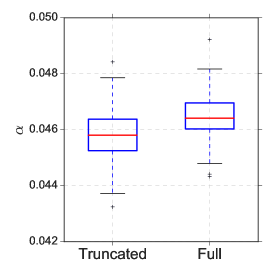
(b) Noise level $=10\%$

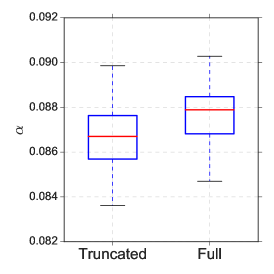
(c) Noise level $=25\%$

Figure 5. Box plots comparing parameter estimates $\alpha_{k_{\mathrm{opt}}}$ with $\alpha_{r}$ for problem Satellite computed from $100$ runs for noise levels $5\%$, $10\%$, and $25\%$. For each noise level, the estimate $\alpha_{k_{\mathrm{opt}}}$ produced by Algorithm 1 is generally less than $\alpha_{r}$, demonstrating that by including more terms in the TSVD, $k>k_{\mathrm{opt}}$, greater regularization is required. Note that the limits on the $y-$axes vary across subplots to better visualize the parameter distributions across noise levels.

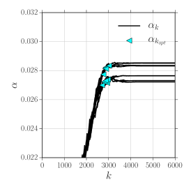
(a) Noise level $=5\%$

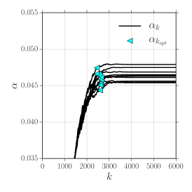
(b) Noise level $=10\%$

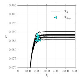
(c) Noise level $=25\%$

Figure 6. Line plots showing the calculated estimates for $\{\alpha_{k}\}$ with increasing number of terms $k$ in the TSVD. The results are given for problem Satellite for noise levels $5\%$, $10\%$, and $25\%$, for $10$ random noise instances at the specified noise level. The resulting point $(k_{\mathrm{opt}},\alpha_{k_{\mathrm{opt}}})$ produced by Algorithm 1 is displayed as a cyan triangle. Note that the limits on the $y-$axes vary across subplots to better visualize the convergence across noise levels.

Figure  4 is a box plot showing the spread of $k_{\mathrm{opt}}$ values for the $100$ noise instances run for each noise level, where in each case $k_{\mathrm{opt}}\ll r=65536$. Figure 5 is a box plot comparing the $\alpha_{k_{\mathrm{opt}}}$ returned by the algorithm, and $\alpha_{r}$ obtained by minimizing the UPRE on the full space. These figures together reaffirm that the optimal regularization parameter found by UPRE is largely determined by a relatively small number of terms in the TSVD, and less impacted by the tail of the coefficients dominated by noise. The estimation of $\{\alpha_{k}\}$ with increasing number of terms in the TSVD is depicted in Figure 6 for the first $10$ runs of each noise level, where the point of convergence $(k_{\mathrm{opt}},\alpha_{k_{\mathrm{opt}}})$ is represented as a cyan triangle. It should be noted that the estimated lower bound $\alpha_{\mathrm{min}}$ was not used, and $\alpha$ was minimized over the interval $(0,1)$ using fminbnd (fminbound is used for the Python implementation). A tolerance of $\delta=1\mathrm{e}{-3}$ was found to produce a value for $\alpha_{k_{\mathrm{opt}}}$ just prior to the point where $\{\alpha_{k}\}$ began to stabilize. A smaller $\delta$ will necessarily increase $k_{\mathrm{opt}}$, but with negligible changes in $\alpha_{k_{\mathrm{opt}}}$. In these simulations averaged over all $100$ runs, $\alpha_{k_{\mathrm{opt}}}$ was within $1.22\%$, $1.47\%$, and $1.17\%$ of $\alpha_{r}$ for noise levels $5\%$, $10\%$, and $25\%$ respectively using fewer than $5\%$ of the SVD components.

In terms of RRE, the solution obtained using the truncated UPRE and a subspace of size $k_{\mathrm{opt}}$ with parameter $\alpha_{k_{\mathrm{opt}}}$ generated by Algorithm 1 generally provided a better solution than obtained using the full UPRE for each noise level. Figures 7 and  8 show box plots and histograms respectively of the RRE comparing the regularized TSVD and the full UPRE solution. Over all noise levels, the median and mean reconstruction error of $100$ noise instances is lower in the regularized TSVD solution. Similar to the Picard parameter approaches of [34], Algorithm 1 identifies an index $k_{\mathrm{opt}}$ for which coefficients $s_{k}$ are dominated by noise for $k>k_{\mathrm{opt}}$. Our approach, however, does not rely on performing statistical tests on the coefficients, but instead examines the stabilization of $\alpha_{k}$ as $k$ increases. Once $\alpha_{k}$ has stabilized, adding additional noise dominated terms in the solution delivers no benefit. Furthermore, if a TSVD with $k_{\mathrm{max}}$ terms has been calculated, then either $\alpha_{k}$ converges for $k<k_{\mathrm{max}}$ or we know that the optimal choice $k_{\mathrm{opt}}$ is greater than $k_{\mathrm{max}}$, and that $\hat{c}_{iw}$ provides some estimate for whether $k_{\mathrm{opt}}>>k_{\mathrm{max}}$ or whether the given TSVD can be assumed to be sufficient in providing a good estimate for the solution $\mathbf{x}$.

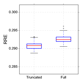
(a) Noise level $=5\%$

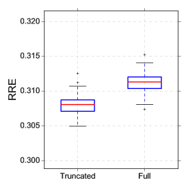
(b) Noise level $=10\%$

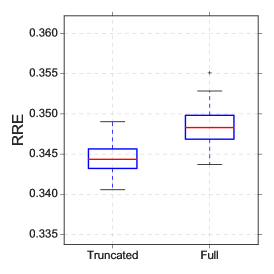
(c) Noise level $=25\%$

Figure 7. Box plots of RRE comparing solutions using truncated UPRE with parameter $\alpha_{k_{\mathrm{opt}}}$ and solutions using full UPRE with parameter $\alpha_{r}$ for problem Satellite computed from $100$ runs for noise levels $5\%$, $10\%$, and $25\%$. Regularization parameter $\alpha_{kopt}$ obtained by UPRE on a TSVD generally has lower error, as evident from Truncated UPRE plots being vertically shifted downwards relative to full UPRE boxplots. Note that the limits on the $y-$axes vary across subplots to better visualize the spread of the distributions across noise levels.

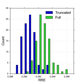
(a) Noise level $=5\%$

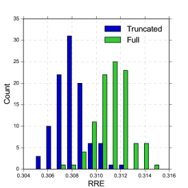
(b) Noise level $=10\%$

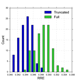
(c) Noise level $=25\%$

Figure 8. Histograms of RRE comparing solutions using $\alpha_{k_{\mathrm{opt}}}$ and solutions using $\alpha_{r}$ for problem Satellite computed from $100$ runs for each noise level $5\%$, $10\%$, and $25\%$. Regularization parameter $\alpha_{k_{\mathrm{opt}}}$ obtained by UPRE on a TSVD generally has lower error, as evident from the truncated histograms having peaks shifted to the left relative to the full UPRE.

In these simulations $\ell$ is not known precisely but was estimated by visual inspection of the Picard coefficients, as well as by comparing the distributions of the noise contaminated and noise free coefficients. This approach for estimating $\ell$ is not possible in general as the noise free coefficients are unknown in practice, but this method of estimating $\ell$ was employed for the purpose of validating the results of Theorem 3.1. An estimate for the lower bound $\alpha_{\mathrm{min}}$ obtained from (29) is depicted as the red dashed curve in Figure 9, with $\{\alpha_{k}\}$ the solid black line. It can be seen that $\alpha_{\mathrm{min}}$ serves as a tight lower bound for the converged parameter $\alpha_{k_{\mathrm{opt}}}$, and the lower bound $\sigma_{k+1}/\sqrt{1-\sigma_{k+1}^{2}}$ can be used effectively in cases where an estimate of $\ell$ is not available.

In addition to test image Satellite with a medium Gaussian blur applied, we also applied Algorithm 1 with the same parameters to test image HST with both mild and severe Gaussian blurring. The results, summarized in Figures 10 - 12 are consistent with the results for test case Satellite.

In summary, given a TSVD or SVD, an optional estimate of $\ell$, and suitable parameters determined by the ill-posedness of the problem, Algorithm 1 is able to effectively determine a regularization parameter $\alpha_{k_{\mathrm{opt}}}$ obtained by UPRE minimization over the TSVD subspace of size $k_{\mathrm{opt}}$, such that the regularized truncated solution $\bf x$ has consistently lower RRE than the full UPRE solution.

(a) Noise $=5\%$

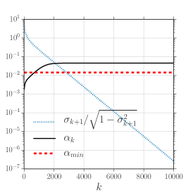
(b) Noise $=10\%$

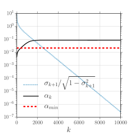
(c) Noise $=25\%$

Figure 9. Line plots showing the convergence of $\{\alpha_{k}\}$ for problem Satellite for noise levels $5\%$, $10\%$, and $25\%$. In each subplot, $\alpha_{r}$ is plotted as a solid black line for $10$ random noise instances at the specified noise level. The dotted blue curve represents the lower bound in (29) as a function of $k$, with the red dashed line representing the lower bound according to Theorem 3.1 and dependent on $\ell$ for a single run.

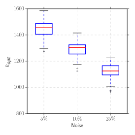
(a) HST severe blurring

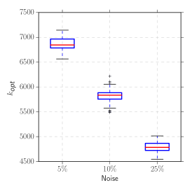
(b) HST mild blurring

Figure 10. Box plots showing the index $k_{\mathrm{opt}}$ produced by Algorithm 1 for problem HST computed from $100$ runs for noise levels $5\%$, $10\%$, and $25\%$. The number of terms $k$ in the TSVD that provide useful information decreases as the noise level increases.

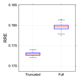
(a) Noise level $=5\%$

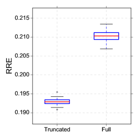
(b) Noise level $=10\%$

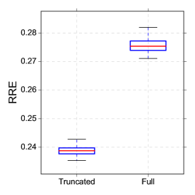
(c) Noise level $=25\%$

Figure 11. Box plots of RRE comparing solutions using truncated UPRE with parameter $\alpha_{k_{\mathrm{opt}}}$ and solutions using full UPRE with parameter $\alpha_{r}$ for problem HST with mild blur computed from $100$ runs for noise levels $5\%$, $10\%$, and $25\%$. Regularization parameter $\alpha_{k_{\mathrm{opt}}}$ obtained by UPRE on a TSVD has consistent lower error, as evident from Truncated UPRE plots being vertically shifted downwards relative to full UPRE boxplots. Note that the limits on the $y-$axes vary across subplots to better visualize the spread of the distributions across noise levels.

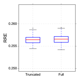
(a) Noise level $=5\%$

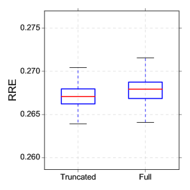
(b) Noise level $=10\%$

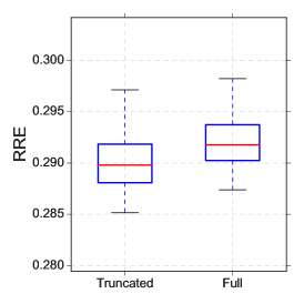
(c) Noise level $=25\%$

Figure 12. Box plots of RRE comparing solutions using truncated UPRE with parameter $\alpha_{k_{\mathrm{opt}}}$ and solutions using full UPRE with parameter $\alpha_{r}$ for problem HST with severe blur computed from $100$ runs for noise levels $5\%$, $10\%$, and $25\%$. Regularization parameter $\alpha_{k_{\mathrm{opt}}}$ obtained by UPRE on a TSVD generally has lower error for noise levels $10\%$ and $25\%$, with comparable error for noise level $5\%$. Note that the limits on the $y-$axes vary across subplots to better visualize the spread of the distributions across noise levels.

5. Conclusions

We have demonstrated that the regularization parameter obtained using the UPRE estimator converges with increasing number of terms used from the TSVD for the solution. For a severely ill-posed problem the convergence occurs very quickly and is independent of the size of the problem due to the fast contamination of data coefficients by practical levels of noise. Practically-relevant problems are often, however, only moderately or mildly ill-posed, e. g. [6, 14, 36, 38], and it is therefore important to accurately and efficiently find both $k_{\mathrm{opt}}$ and $\alpha_{k_{\mathrm{opt}}}$.

Theoretical results have been presented that demonstrate the convergence of the regularization parameter $\alpha_{k}$ with $k$, increasing from below to $\alpha_{k_{\mathrm{opt}}}\leq\alpha_{r}$, the optimal value for the full SVD. The posterior covariance thus decreases with $k$, leveling at approximately $\sigma^{2}/(4\alpha_{k_{\mathrm{opt}}}^{2})$. Thus the method naturally finds a solution which has increasing smoothness with increasing $k$ and solutions obtained without truncation will exhibit larger error due to increased smoothing. An effective and practical algorithm that implements the theory has also been provided, and validated for $2$D image deblurring. These results expand on recent research on the characterization of the regularization parameter as closely dependent on the size of the singular subspace represented in the solution, [9, 30, 31]. As there is a resurgence of interest in using a TSVD solution for the solution of ill-posed problems due to increased feasibility of finding a good approximation of a dominant singular subspace using techniques from randomization, e.g. [7, 8, 13, 26, 28, 32], the results are more broadly relevant for more efficient estimates of the TSVD. Implementation of the algorithm in these contexts is a topic for future work.

References

- [1] J.-F. P. J. Abascal, S. R. Arridge, R. H. Bayford, and D. S. Holder, Comparison of methods for optimal choice of the regularization parameter for linear electrical impedance tomography of brain function., Physiol Meas, 29 (2008), pp. 1319–1334.
- [2] R. C. Aster, B. Borchers, and C.H. Thurber, Parameter Estimation and Inverse Problems, Elsevier, Amsterdam, 2nd. ed., 2013.
- [3] A. B. Bakushinskii, Remarks on choosing a regularization parameter using the quasi-optimality and ratio criterion, USSR Comp. Math. Math. Phys. 24(4), (1984), 181182 .
- [4] F. Bauer and M. A. Lukas, Comparing parameter choice methods for regularization of ill-posed problems, Mathematics and Computers in Simulation, 81 (2011), pp. 1795 – 1841.
- [5] A. Björck, Numerical Methods for Least Squares Problems, Society for Industrial and Applied Mathematics, Philadelphia, 1996.
- [6] J. Chung, J. G. Nagy, and D. P. O’Leary, A weighted GCV method for Lanczos hybrid regularization, Electronic Transactions on Numerical Analysis, 28 (2008), pp. 149–167.
- [7] P. Drineas and M. W. Mahoney, RandNLA: Randomized numerical linear algebra, Communications of the ACM, 59 (2016), pp. 80–90.
- [8] P. Drineas, M. W. Mahoney, S. Muthukrishnan, and T. Sarlós, Faster least squares approximation, Numerische Mathematik, 117 (2011), pp. 219–249.
- [9] C. Fenu, L. Reichel, G. Rodrigues, and H. Sadok, GCV for Tikhonov regularization by partial SVD, BIT Numerical Mathematics, 57 (2017), pp. 1019–1039.
- [10] S. Gazzola, P. C. Hansen, and J. G. Nagy. IR Tools: a MATLAB package of iterative regularization methods and large-scale test problems, Numerical Algorithms. https://doi.org/10.1007/s11075-018-0570-7.2018.
- [11] G. H. Golub, M. Heath, and G. Wahba, Generalized cross-validation as a method for choosing a good ridge parameter, Technometrics, 21 (1979), pp. 215–223.
- [12] G. H. Golub and C. F. van Loan, Matrix computations, Johns Hopkins Press, Baltimore, 3rd ed., 1996.
- [13] R. M. Gower and P. Richtárik, Randomized iterative methods for linear systems, SIAM Journal on Matrix Analysis and Applications, 36 (2015), pp. 1660–1690.
- [14] K. Hämäläinen, L. Harhanen, A. Kallonen, A. Kujanpää, E. Niemi, and S. Siltanen, Tomographic X-ray data of a walnut, arXiv:1502.04064, (2015).
- [15] U. Hämarik, R. Palm, and T. Raus, On minimization strategies for choice of the regularization parameter in ill-posed problems, Numerical Functional Analysis and Optimization, 30 (2009), pp. 924–950.
- [16] U. Hämarik, R. Palm, and T. Raus, A family of rules for parameter choice in Tikhonov regularization of ill-posed problems with inexact noise level, Journal of Computational and Applied Mathematics, 236 (2012), pp. 2146 – 2157. Inverse Problems: Computation and Applications.
- [17] M. Hanke and P. C. Hansen, Regularization methods for large-scale problems, Survey on Mathematics for Industry, 3 (1993), pp. 253–315.
- [18] J. K. Hansen, J. D. Hogue, G. K. Sander, R. A. Renaut, and S. C. Popat, Non-negatively constrained least squares and parameter choice by the residual periodogram for the inversion of electrochemical impedance spectroscopy data, Journal of Computational and Applied Mathematics, 278 (2015), pp. 52 – 74.
- [19] P. C. Hansen, The discrete Picard condition for discrete ill-posed problems, BIT Numerical Mathematics, 30 (1990), pp. 658–672.
- [20] P. C. Hansen, Regularization tools – a Matlab package for analysis and solution of discrete ill-posed problems, Numerical Algorithms, 46 (1994), pp. 189–194.
- [21] , Rank-Deficient and Discrete Ill-Posed Problems, Society for Industrial and Applied Mathematics, Philadelphia, 1998.
- [22] P. C. Hansen, Discrete Inverse Problems, Society for Industrial and Applied Mathematics, Philadelphia, 2010.
- [23] B. Hofmann, Regularization for applied inverse and ill-posed problems: a numerical approach, Teubner-Texte zur Mathematik, B.G. Teubner, 1986.
- [24] E. Levin and A. Y. Meltzer, Estimation of the regularization parameter in linear discrete ill-posed problems using the Picard parameter, SIAM Journal on Scientific Computing, 39 (2017), pp. A2741–A2762.
- [25] Y. Lin, B. Wohlberg, and H. Guo, UPRE method for total variation parameter selection, Signal Processing, 90 (2010), pp. 2546–2551.
- [26] M. W. Mahoney, Randomized algorithms for matrices and data, Foundations and Trends® in Machine Learning, 3 (2011), pp. 123–224.
- [27] J. L. Mead and R. A. Renaut, A Newton root-finding algorithm for estimating the regularization parameter for solving ill-conditioned least squares problems, Inverse Problems, 25 (2009), p. 025002.
- [28] X. Meng, M. A. Saunders, and M. W. Mahoney, LSRN: A parallel iterative solver for strongly over- or underdetermined systems, SIAM Journal on Scientific Computing, 36 (2014), pp. C95–C118.
- [29] V. A. Morozov, On the solution of functional equations by the method of regularization, Sov. Math. Dokl., 7 (1966), pp. 414–417.
- [30] R. A. Renaut, M. Horst, Y. Wang, D. Cochran, and J. Hansen, Efficient estimation of regularization parameters via downsampling and the singular value expansion, BIT Numerical Mathematics, 57 (2017), pp. 499–529.
- [31] R. A. Renaut, S. Vatankhah, and V. E. Ardestani, Hybrid and iteratively reweighted regularization by unbiased predictive risk and weighted GCV for projected systems, SIAM Journal on Scientific Computing, 39 (2017), pp. B221–B243.
- [32] V. Rokhlin and M. Tygert, A fast randomized algorithm for overdetermined linear least-squares regression, Proceedings of the National Academy of Sciences, 105 (2008), pp. 13212–13217.
- [33] C. M. Stein, Estimation of the mean of a multivariate normal distribution, Ann. Statist., 9 (1981), pp. 1135–1151.
- [34] V. Taroudaki and D. P. O’Leary, Near-optimal spectral filtering and error estimation for solving ill-posed problems, SIAM Journal on Scientific Computing, 37 (2015), pp. A2947–A2968.
- [35] A. Toma, B. Sixou, and F. Peyrin, Iterative choice of the optimal regularization parameter in tv image restoration, Inverse Problems & Imaging, 9 (2015), p. 1171.
- [36] S. Vatankhah, V. E. Ardestani, and R. A. Renaut, Automatic estimation of the regularization parameter in 2D focusing gravity inversion: application of the method to the Safo manganese mine in the northwest of Iran, Journal of Geophysics and Engineering, 11 (2014), p. 045001.
- [37] , Application of the principle and unbiased predictive risk estimator for determining the regularization parameter in 3-D focusing gravity inversion, Geophysical Journal International, 200 (2015), pp. 265–277.
- [38] S. Vatankhah, R. A. Renaut, and V. E. Ardestani, 3-D projected inversion of gravity data using truncated unbiased predictive risk estimator for regularization parameter estimation, Geophysical Journal International, 210 (2017), pp. 1872–1887.
- [39] , A fast algorithm for regularized focused 3-D inversion of gravity data using the randomized SVD, Geophysics, (2018).
- [40] S. Vatankhah, R. A. Renaut, and V. E. Ardestani, Total variation regularization of the 3-d gravity inverse problem using a randomized generalized singular value decomposition, Geophysical Journal International, 213 (2018), pp. 695–705.
- [41] C. Vogel, Computational Methods for Inverse Problems, Society for Industrial and Applied Mathematics, Philadelphia, 2002.