A CONSTRUCTION OF GRAPHS WITH POSITIVE RICCI CURVATURE

Abstract.

Two complete graphs are connected by adding some edges. The obtained graph is called the gluing graph. The more we add edges, the larger the Ricci curvature on it becomes. We calculate the Ricci curvature of each edge on the gluing graph and obtain the least number of edges that result in the gluing graph having positive Ricci curvature.

1. Introduction

The Ricci curvature is one of the most important concepts in Riemannian geometry. There are some definitions for the generalized Ricci curvature, and Ollivier’s coarse Ricci curvature is one of them (see [5]). It is formulated using the Wasserstein distance on a metric space $(X,d)$ with a random walk $m=\left\{m_{x}\right\}_{x\in X}$, where each $m_{x}$ is a probability measure on $X$. The coarse Ricci curvature is defined as follows: For two distinct points $x,y\in X$,

$$\kappa(x,y):=1-\cfrac{W(m_{x},m_{y})}{d(x,y)},$$

where $W$($m_{x},m_{y}$) is the $1$-Wasserstein distance between $m_{x}$ and $m_{y}$. This definition was applied to graphs in the year 2010 and many researchers are focused on this.
　In 2010, Lin-Lu-Yau [4] defined the Ricci curvature of an undirected graph by using the coarse Ricci curvature of the lazy random walk. They studied the Ricci curvature of the product space of graphs and random graphs. They also considered a graph of positive Ricci curvature and proved some properties. In 2012, Jost and Liu [3] studied the relationship between the coarse Ricci curvature of the simple random walk and the local clustering efficient. In this paper, the coarse Ricci curvature is simply called the Ricci curvature. Given that we obtain several global properties on graphs with positive Ricci curvature by their results, we would like to constitute a new graph with positive Ricci curvature. A complete graph $K_{n}$ is one of graphs with positive Ricci curvature. In fact, we have $\kappa(x,y)=(n-2)/(n-1)$ for any edge $(x,y)\in E(K_{n})$. Therefore, in this paper, we start from two complete graphs $K_{n}$ and $K^{\prime}_{n}$, and connect them by several edges. For the obtained graph that is called the $m$-gluing graph (See Definition 3.1), we obtain the following theorem regarding the minimal number of $m$ satisfying the condition that the $m$-gluing graph must have positive Ricci curvature.

Theorem 1.1.

For the $m$-gluing graph $K_{n}+_{m}K^{\prime}_{n}$ of two complete graphs $K_{n}$ and $K^{\prime}_{n}$, $n\geq 5$, we have $\kappa(x,y)>0$ for any edge $(x,y)\in E$ if and only if

$$\cfrac{n^{2}-2n}{n+2}<m\leq n-1.$$

If we calculate the Ricci curvature of edges on the $m$-gluing graph by the estimates of known results (see Theorem 2.9 and Theorem 2.10), then there exist several edges such that the estimate of either Theorem 2.9 or Theorem 2.10 is not optimal (see Remark 3.4 and Remark 3.8). Thus we calculate the Ricci curvature of each edge based on the definition of the Ricci curvature.
　In the last section, we obtain some estimates of the eigenvalues of the normalized graph Laplacian and the Cheeger constant by the Ricci curvature on the $m$-gluing graph.

2. Ricci curvature

In this paper, we assume that $G=(V,E)$ is an undirected connected simple finite graph, where $V$ is the set of the vertices and $E$ the set of edges. That is,

1. for any two vertices, there exists a path connecting them,

2. there exists no loop and no multiple edges,

3. and the number of vertices and edges is finite.

For $x,y\in V$, we write $(x,y)$ as an edge from $x$ to $y$. We denote the set of vertices of a graph $H$ by $V(H)$ and the set of edges of $H$ by $E(H)$.

Definition 2.1.

1. A path from a vertex $x\in V$ to a vertex $y\in V$ is a sequence of edges $\left\{(a_{i},a_{i+1)}\right\}_{i=0}^{n-1}$, where $a_{0}=x$, $a_{n}=y$. We call $n$ the length of the path.

2. The distance $d(x,y)$ between two vertices $x,y\in V$ is given by the length of a shortest path between $x$ and $y$.

3. The diameter of $G$, denoted by $\operatorname{diam}G$, is given by the maximum of the distance between any two vertices on $G$.

Definition 2.2.

1. For any $x\in V$, the neighborhood of $x$ is defined as

   $$\Gamma(x):=\left\{y\in V\mid(x,y)\in E\right\}.$$

2. For any $x\in V$, the degree of $x$, denoted by $d_{x}$, is the number of edges starting from $x$.

3. If every vertex has the same degree $d$, then we call $G$ a $d$-regular graph.

Definition 2.3.

For any vertex $x\in V$, we define a probability measure $m_{x}$ on $V$ by

$$m_{x}(v)=\begin{cases}\cfrac{1}{d_{x}},&\mathrm{if}\ (x,v)\in E,\\ 0,&\mathrm{\mathrm{otherwise}}.\end{cases}$$

$m=\left\{m_{x}\right\}_{x\in V}$ is called the simple random walk.

To define the Ricci curvature, we define the 1-Wasserstein distance as follows:

Definition 2.4.

The 1-Wasserstein distance between any two probability measures $\mu$ and $\nu$ on $V$ is given as follows

$$W(\mu,\nu)=\inf_{A}\sum_{u,v\in V}A(u,v)d(u,v),$$

where $A:V(G)\times V(G)\to[0,1]$ runs over all maps satisfying

(2.1) $$\begin{cases}\sum_{v\in V}A(u,v)=\mu(u),\\ \sum_{u\in V}A(u,v)=\nu(v).\end{cases}$$

Such a map $A$ is called a coupling between $\mu$ and $\nu$.

Remark 2.5.

There exists a coupling $A$ that attains the 1-Wasserstein distance (see [2], [6] and [7]), and we call it an optimal coupling.

One of the most important properties of the 1-Wasserstein distance is the Kantorovich-Rubinstein duality, which is stated as follows:

Proposition 2.6 (Kantorovich, Rubinstein).

The 1-Wasserstein distance between any two probability measures $\mu$ and $\nu$ on $V$ is written as

$$W(\mu,\nu)=\sup_{f}\sum_{u\in V}f(u)(\mu(u)-\nu(u)),$$

where the supremum is taken over all functions on $G$ that satisfy $|f(u)-f(v)|\leq d(u,v)$ for any $u,v\in V$.

A function $f$ on $V$ is said to be $1$-Lipschitz if $|f(u)-f(v)|\leq d(u,v)$ for any $u,v\in V$.

Definition 2.7.

For any two distinct vertices $x,y\in V$, the Ricci curvature of $x$ and $y$ is defined as follows:

$$\kappa(x,y)=1-\cfrac{W(m_{x},m_{y})}{d(x,y)}.$$

Whenever we are interested in a lower bound of Ricci curvature, the following lemma implies that it is sufficient to consider the Ricci curvature of the edge, although the Ricci curvature is defined for any pair of vertices.

Proposition 2.8 (Lin-Lu-Yau, [4]).

If $\kappa(u,v)\geq k$ for any edge $(u,v)\in E$ and for a real number $k$, then $\kappa(x,y)\geq k$ for any pair of vertices $(x,y)\in V\times V$.

To calculate the Ricci curvature, Jost and Liu gave the following estimate of the Ricci curvature.

Theorem 2.9 (Jost-Liu [3]).

On a locally finite graph, for any pair of neighboring vertices $x$ and $y$, we have

$$\kappa(x,y)\geq-\left(1-\cfrac{1}{d_{x}}-\cfrac{1}{d_{y}}-\cfrac{\#(x,y)}{d_{x}\wedge d_{y}}\right)_{+}-\left(1-\cfrac{1}{d_{x}}-\cfrac{1}{d_{y}}-\cfrac{\#(x,y)}{d_{x}\vee d_{y}}\right)_{+}+\cfrac{\#(x,y)}{d_{x}\vee d_{y}},$$

where $\#(x,y)$ is the number of triangles which includes $x,y$ as vertices, and $s_{+}:=\max(s,0)$, $s\vee t:=\max(s,t)$, and $s\wedge t:=\min(s,t)$ for real numbers $s$ and $t$.

Theorem 2.10 (Jost-Liu [3]).

On a locally finite graph, for any pair of neighboring vertices $x$ and $y$, we have

$$\kappa(x,y)\leq\cfrac{\#(x,y)}{d_{x}\vee d_{y}}.$$

3. Proof of the main result

Let $K_{n}$ and $K^{\prime}_{n}$ be complete graphs, where $V(K_{n})=\left\{u_{0},u_{1},\cdots,u_{n-1}\right\}$ and $V(K^{\prime}_{n})=\left\{v_{0},v_{1},\cdots,v_{n-1}\right\}$. Before we prove Theorem 1.1, we define the $m$-gluing graph of $K_{n}$ and $K^{\prime}_{n}$ as follows:

Definition 3.1.

The $m$-gluing graph of two complete graphs $K_{n}$ and $K^{\prime}_{n}$, denoted by $K_{n}+_{m}K^{\prime}_{n}$, is defined by the following.

1. The vertex set $V(K_{n}+_{m}K^{\prime}_{n})=V(K_{n})\cup V(K^{\prime}_{n})$.

2. The edge set $E(K_{n}+_{m}K^{\prime}_{n})=E(K_{n})\cup E(K^{\prime}_{n})\cup\left\{(u_{0},v_{0})\right\}\cup\left\{(u_{0},v_{i})\mid 1\leq i\leq m\right\}\cup\left\{(u_{j},v_{0})\mid 1\leq j\leq m\right\}$.

We denote $\left\{v_{i}\in V(K^{\prime}_{n})\mid 1\leq i\leq m\right\}$ and $\left\{u_{j}\in V(K_{n})\mid 1\leq j\leq m\right\}$ by $\Gamma_{m}(u_{0})$ and $\Gamma_{m}(v_{0})$, respectively.

3.1. Proof of Theorem 1.1 in the case of $\bf m=n-1$

To obtain the value of $\kappa(x,y)$ on any edge $(x,y)\in E(K_{n}+_{n-1}K^{\prime}_{n})$, it is sufficient to calculate $\kappa(u_{0},v_{0})$, $\kappa(u_{0},v_{1})$, $\kappa(u_{0},u_{1})$, and $\kappa(u_{1},u_{2})$ by the symmetry of the $m$-gluing graph. Thus, combining Theorem 3.2 and Proposition 3.3, we obtain $\kappa(x,y)>0$ for any edge $(x,y)\in E(K_{n}+_{n-1}K^{\prime}_{n})$.

Theorem 3.2.

Regarding the gluing graph $K_{n}+_{n-1}K^{\prime}_{n}$, we have

1. $\kappa(u_{1},u_{2})=\cfrac{n-1}{n}$,

2. $\kappa(u_{0},v_{0})=\cfrac{2n-2}{2n-1}$,

3. $\kappa(u_{0},v_{1})=\cfrac{3n-2}{n(2n-1)}$.

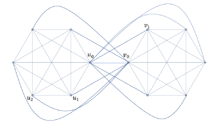
Figure 1. $K_{6}+_{5}K_{6}$

Proof..

Given that (1) and (2) are held by using Theorem 2.9 and Theorem 2.10, it is sufficient to prove only (3). To calculate the Ricci curvature on $(u_{0},v_{1})$, we define a map $B_{3}:V\times V\to\mathbb{R}$ by

$$B_{3}(x,y)=\begin{cases}\cfrac{1}{2n-1},&\mathrm{if}\ x=y\in\Gamma(u_{0})\cap\Gamma(v_{1}),\\ \cfrac{1}{(n-2)(2n-1)},&\mathrm{if}\ x=v_{1},y\in\Gamma_{n-1}(u_{0})\setminus\left\{v_{1}\right\},\\ \cfrac{1}{n(n-1)},&\mathrm{if}\ x\in\Gamma_{n-1}(v_{0}),y=u_{0},\\ \cfrac{1}{n-1}\left(\cfrac{1}{n}-\cfrac{1}{2n-1}\right),&\mathrm{if}\ x\in\Gamma_{n-1}(v_{0}),y=v_{0},\\ \cfrac{1}{n-1}\left\{\left(\cfrac{1}{n}-\cfrac{1}{2n-1}\right)-\cfrac{1}{(n-2)(2n-1)}\right\},&\mathrm{if}\ x\in\Gamma_{n-1}(v_{0}),y\in\Gamma_{n-1}(u_{0})\setminus\left\{v_{1}\right\},\\ 0,&\mathrm{otherwise}.\end{cases}$$

This map is a coupling between $m_{u_{0}}$ and $m_{v_{1}}$. In fact, we have

$$\sum_{x\in V}B_{3}(x,v_{j}) = \cfrac{1}{2n-1}+\cfrac{1}{(n-2)(2n-1)}+\left\{\left(\cfrac{1}{n}-\cfrac{1}{2n-1}\right)-\cfrac{1}{(n-2)(2n-1)}\right\}$$

$$= \cfrac{1}{n},$$

$$\sum_{y\in V}B_{3}(u_{i},y) = \cfrac{1}{n(n-1)}+\cfrac{1}{n-1}\left(\cfrac{1}{n}-\cfrac{1}{2n-1}\right)$$

$$+ \cfrac{n-2}{n-1}\left\{\left(\cfrac{1}{n}-\cfrac{1}{2n-1}\right)-\cfrac{1}{(n-2)(2n-1)}\right\}$$

$$= \cfrac{1}{2n-1}.$$

The others are obvious. Then, the 1-Wasserstein distance is estimated as follows:

$$W(m_{u_{0}},m_{v_{1}}) \leq \cfrac{1}{n}+\left(\cfrac{1}{n}-\cfrac{1}{2n-1}\right)+\cfrac{1}{2n-1}$$

$$+ (n-2)\left\{\left(\cfrac{1}{n}-\cfrac{1}{2n-1}\right)-\cfrac{1}{(n-2)(2n-1)}\right\}$$

$$= \cfrac{2n-2}{n}-\cfrac{2n-2}{2n-1}.$$

On the other hand, we define a function $f:V\to\mathbb{R}$ by

$$f(w)=\begin{cases}-2,&\mathrm{if}\ w\in\Gamma_{n-1}(u_{0})\setminus\left\{v_{1}\right\},\\ -1,&\mathrm{if}\ w\in\left\{u_{0},v_{1},v_{0}\right\},\\ 0,&\mathrm{otherwise}.\end{cases}$$

It is easy to show that $f$ is a 1-Lipschitz function. By Proposition 2.6, the 1-Wasserstein distance is estimated as follows:

$$W(m_{u_{0}},m_{v_{1}}) \geq (n-2)\left\{2\times\left(\cfrac{1}{n}-\cfrac{1}{2n-1}\right)\right\}+\cfrac{1}{n}-\cfrac{1}{2n-1}+\left(\cfrac{1}{n}-\cfrac{1}{2n-1}\right)$$

$$= (2n-2)\left(\cfrac{1}{n}-\cfrac{1}{2n-1}\right).$$

Thus we obtain

$$W(m_{u_{0}},m_{v_{1}})=(2n-2)\left(\cfrac{1}{n}-\cfrac{1}{2n-1}\right)=\cfrac{2(n-1)^{2}}{n(2n-1)},$$

which implies $\kappa(u_{0},v_{1})=(3n-2)/\left\{n(2n-1)\right\}$. This completes the proof. ∎

For the edge $(u_{0},u_{1})$, we calculate the Ricci curvature for $m\leq n-1$.

Proposition 3.3.

For any vertex $u\in\Gamma_{m}(v_{0})$, we have

$$\kappa(u_{0},u)=\begin{cases}\cfrac{n-1}{n+1},&\mathrm{if}\ m=1,\\ \cfrac{n^{2}-mn+2m}{n(n+m)},&\mathrm{if}\ m\geq 2.\end{cases}$$

Proof..

We take the vertex $u_{1}\in\Gamma_{m}(v_{0})$, and consider the Ricci curvature of $(u_{0},u_{1})$. Given that the case of $m=1$ is held by using Theorem 2.9 and 2.10, we consider the case of $m\geq 2$. We define a map $A:V\times V\to\mathbb{R}$ by

$$A(x,y)=\begin{cases}\cfrac{1}{n+m},&\mathrm{if}\ x=y\in\Gamma(u_{0})\cap\Gamma(u_{1}),\\ \cfrac{1}{nm},&\mathrm{if}\ x\in\Gamma_{m}(u_{0}),y=u_{0},\\ \cfrac{1}{m}\left(\cfrac{1}{n}-\cfrac{1}{n+m}\right),&\mathrm{if}\ x\in\Gamma_{m}(u_{0}),y=v_{0},\\ \cfrac{1}{(n-2)(n+m)},&\mathrm{if}\ x=u_{1},y\in V(K_{n})\setminus\left\{u_{0},u_{1}\right\},\\ \cfrac{1}{m}\left\{\left(\cfrac{1}{n}-\cfrac{1}{n+m}\right)-\cfrac{1}{(n-2)(n+m)}\right\},&\mathrm{if}\ x\in\Gamma_{m}(u_{0}),y\in V(K_{n})\setminus\left\{u_{0},u_{1}\right\},\\ 0,&\mathrm{otherwise}.\end{cases}$$

This map is a coupling between $m_{u_{0}}$ and $m_{u_{1}}$. Then, the 1-Wasserstein distance is estimated as follows:

$$W(m_{u_{0}},m_{u_{1}}) \leq \cfrac{1}{n}+\left(\cfrac{1}{n}-\cfrac{1}{n+m}\right)+\cfrac{1}{n+m}$$

$$+ 2(n-2)\left\{\left(\cfrac{1}{n}-\cfrac{1}{n+m}\right)-\cfrac{1}{(n-2)(n+m)}\right\}$$

$$= \cfrac{2n-2}{n}-\cfrac{2n-2}{n+m}=1-\cfrac{n^{2}-mn+2m}{n(n+m)}.$$

On the other hand, we define a function $f_{3}$ by

$$f_{3}(w)=\begin{cases}-2,&\mathrm{if}\ w\in V(K_{n})\setminus\left\{u_{0},u_{1}\right\},\\ -1,&\mathrm{if}\ w\in\left\{u_{0},u_{1},v_{0}\right\},\\ 0,&\mathrm{otherwise}.\end{cases}$$

It is easy to show that $f_{3}$ is a 1-Lipschitz function. By using Proposition 2.6, the 1-Wasserstein distance is estimated as follows:

$$W(m_{u_{0}},m_{u_{1}}) \geq -2(n-2)\left(\cfrac{1}{n+m}-\cfrac{1}{n}\right)+\cfrac{1}{n}-\cfrac{1}{n+m}+\left(\cfrac{1}{n}-\cfrac{1}{n+m}\right)$$

$$= (2n-2)\left(\cfrac{1}{n}-\cfrac{1}{n+m}\right).$$

This completes the proof. ∎

Remark 3.4.

In the case of $m\geq 2$, if we use Theorem 2.9, then we obtain

$$\kappa(u_{0},u)\geq\cfrac{n^{2}-nm+m}{n(n+m)},$$

for any vertex $u\in\Gamma_{m}(v_{0})$. Therefore, Proposition 3.3 is stronger than Theorem 2.9.

3.2. Proof of Theorem 1.1 in the case of $\bf m\leq n-2$

In the case of $m\leq n-2$, we must calculate the Ricci curvature for 7 edges on $K_{n}+_{m}K^{\prime}_{n}$ using the symmetry of the $m$-gluing graph (see Figure 2). In Figure 2, the Ricci curvature for the edges, as in (3), has already be calculated by using Proposition 3.3. Combining Proposition 3.3, 3.5, 3.7, 3.9, and Corollary 3.10, we obtain Theorem 1.1.

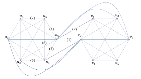
Figure 2. 7 patterns in $K_{6}+_{3}K_{6}$

For the edge (1) in Figure 2, we obtain the following proposition.

Proposition 3.5.

For vertices $u_{0}$ and $v_{0}$, we have

$$\kappa(u_{0},v_{0})=\cfrac{4m-2n+4}{n+m}.$$

In particular, $\kappa(u_{0},v_{0})\geq 0$ if and only if $m\geq(n-2)/2$.

Proof..

By Theorem 2.9, we have

$$W(m_{u_{0}},m_{v_{0}})\leq\cfrac{3n-3m-4}{n+m}.$$

On the other hand, we define a map $f_{1}:V\to\mathbb{R}$ by

$$f_{1}(w)=\begin{cases}3,&\mathrm{if}\ w\in V(K_{n})\setminus(\Gamma_{m}(v_{0})\left\{u_{0}\right\}),\\ 2,&\mathrm{if}\ w\in\left\{u_{0}\right\}\cup\Gamma_{m}(v_{0}),\\ 1,&\mathrm{if}\ w\in\Gamma_{m}(u_{0})\cup\left\{v_{0}\right\},\\ 0,&\mathrm{otherwise}.\end{cases}$$

Since $f_{1}$ is a 1-Lipschitz function, we have

$$W(m_{u_{1}},m_{v_{0}})\geq\cfrac{3}{n+m}(n-m-1)+2\left(-\cfrac{1}{n+m}\right)+\cfrac{1}{n+m}=\cfrac{3n-3m-4}{n+m}.$$

Thus we obtain

$$W(m_{u_{1}},m_{v_{0}})=\cfrac{3n-3m-4}{n+m}=1-\cfrac{4m-2n+4}{n+m}.$$

This completes the proof. ∎

Remark 3.6.

The 1-Lipschitz function defined in the proof of Theorem 2.9 to obtain the upper bound of the Ricci curvature cannot be applied in this case (see [3]); hence, we define the original 1-Lipschitz function $f_{1}$.

For the edge (2) in Figure 2, we obtain the following proposition:

Proposition 3.7.

For any vertex $v\in\Gamma_{m}(u_{0})$, we have

$$\kappa(u_{0},v)=\begin{cases}\cfrac{(2+n)m+2n-n^{2}}{n(n+m)},&\mathrm{if}\ m\geq\cfrac{-n+\sqrt{5n^{2}-8n}}{2},\\ \cfrac{m^{2}+2(n+1)m-2n^{2}+4n}{n(n+m)},&\mathrm{if}\ m<\cfrac{-n+\sqrt{5n^{2}-8n}}{2}.\end{cases}$$

In particular, $\kappa(u_{0},v)>0$ if and only if $m>(n^{2}-2n)/(n+2)$.

Proof..

We take $v_{1}\in\Gamma_{m}(u_{0})$, and consider the Ricci curvature of $(u_{0},v_{1})$. If $m\geq(-n+\sqrt{5n^{2}-4n})/2$, then we define a map $A_{2}:V\times V\to\mathbb{R}$ by

$$A_{2}(x,y)=\begin{cases}\cfrac{1}{n+m},&\mathrm{if}\ x=y\in\Gamma(u_{0})\cap\Gamma(v_{1}),\\ \cfrac{1}{(n-m-1)(n+m)},&\mathrm{if}\ x=v_{1},y\in V(K^{\prime}_{n})\setminus\Gamma_{m}(u_{0}),\\ \cfrac{1}{n(n-m-1)},&\mathrm{if}\ x\in V(K_{n})\setminus\Gamma_{m}(v_{0}),y=u_{0},\\ \cfrac{1}{m-1}\left(\cfrac{1}{n+m}-\cfrac{1}{n(n-m-1)}\right),&\mathrm{if}\ x\in V(K_{n})\setminus\Gamma_{m}(v_{0}),\\ &\ \ \ y\in\Gamma_{m}(u_{0})\setminus\left\{v_{1}\right\},\\ \cfrac{1}{m}\left(\cfrac{1}{n}-\cfrac{1}{n+m}\right),&\mathrm{if}\ x\in\Gamma_{m}(v_{0}),y=v_{0},\\ \cfrac{1}{m}\left(\cfrac{1}{n}-\cfrac{1}{(n-m-1)(n+m)}\right),&\mathrm{if}\ x\in\Gamma_{m}(v_{0}),y\in V(K^{\prime}_{n})\setminus\Gamma_{m}(u_{0}),\\ \cfrac{1}{m}\left\{\cfrac{1}{n}-\cfrac{1}{n+m}-\cfrac{1}{m-1}\left(\cfrac{n-m-1}{n+m}-\cfrac{1}{n}\right)\right\},&\mathrm{if}\ x\in\Gamma_{m}(v_{0}),\ y\in\Gamma_{m}(u_{0})\setminus\left\{v_{1}\right\},\\ 0,&\mathrm{otherwise}.\end{cases}$$

Since $1/(n+m)\geq 1/n(n-m-1)$ is held for $n-3\geq m$, we should assume that $n-3\geq m$, and if $m\geq(-n+\sqrt{5n^{2}-4n})/2$, we have $(n-m-1)/(n+m)-1/n\leq(m-1)(1/n-1/(n+m))$. So, $A_{2}$ is a coupling between $m_{u_{0}}$ and $m_{v_{1}}$. Then the 1-Wasserstein distance is estimated as follows:

$$W(m_{u_{0}},m_{v_{1}}) \leq \cfrac{1}{n+m}+\cfrac{1}{n}+\left(\cfrac{1}{n}-\cfrac{1}{n+m}\right)+2(n-m-1)\left\{\cfrac{1}{n+m}-\cfrac{1}{n(n-m-1)}\right\}$$

$$+ 2\left(\cfrac{n-m-1}{n}-\cfrac{1}{n+m}\right)+2\left\{(m-1)\left(\cfrac{1}{n}-\cfrac{1}{n+m}\right)-\left(\cfrac{n-m-1}{n+m}-\cfrac{1}{n}\right)\right\}$$

$$= \cfrac{2(n^{2}-n-m)}{n(n+m)}.$$

In the case where $m=n-2$, we change the definition of $A_{2}$ to the following:

$$A_{2}(x,y)=\begin{cases}\cfrac{1}{2n-2},&\mathrm{if}\ x=v_{1},\ y=v_{n-1},\\ \cfrac{1}{2n-2},&\mathrm{if}\ x=y\in\Gamma(u_{0})\cap\Gamma(v_{1}),\\ \cfrac{1}{2n-2},&\mathrm{if}\ x=u_{n-1},\ y=u_{0},\\ \cfrac{1}{n-2}\left(\cfrac{1}{n}-\cfrac{1}{2n-2}\right),&\mathrm{if}\ x\in\Gamma_{m}(v_{0}),\ y\in\left\{u_{0},v_{0},v_{n-1}\right\}\cup\Gamma_{m}(u_{0})\setminus\left\{v_{1}\right\},\\ 0,&\mathrm{otherwise}.\end{cases}$$

Then the 1-Wasserstein distance is estimated as follows:

$$W(m_{u_{0}},m_{v_{1}}) \leq \cfrac{1}{2n-2}+\cfrac{1}{2n-2}+\left\{2+2(n-2)\right\}\left(\cfrac{1}{n}-\cfrac{1}{2n-2}\right)=\cfrac{2(n^{2}-2n+2)}{n(n-2)}.$$

Thus, this coincides with the 1-Wasserstein distance in the case of $m\geq n-3$.

On the other hand, we define a map $f_{2}:V\to\mathbb{R}$ by

$$f_{2}(w)=\begin{cases}2,&\mathrm{if}\ w\in V(K_{n})\setminus\left\{u_{0}\right\},\\ 1,&\mathrm{if}\ w\in\left\{u_{0},v_{0},v_{1}\right\},\\ 0,&\mathrm{otherwise}.\end{cases}$$

Given that $f$ is a 1-Lipschitz function, then by the Kantorovich duality, we have the following:

$$W(m_{u_{0}},m_{v_{1}})\geq\cfrac{2(n-1)}{n+m}-\cfrac{2}{n}+\cfrac{2}{n+m}=\cfrac{2(n^{2}-n-m)}{n(n+m)}.$$

Thus we obtain

$$W(m_{u_{0}},m_{v_{1}})=\cfrac{2(n^{2}-n-m)}{n(n+m)}=1-\cfrac{(2+n)m+2n-n^{2}}{n(n+m)}.$$

If $m<(-n+\sqrt{5n^{2}-8n})/2$, then we define a map $A^{\prime}_{2}:V\times V\to\mathbb{R}$ as follows:

$$A^{\prime}_{2}(x,y)=\begin{cases}\cfrac{1}{n+m},&\mathrm{if}\ x=y\in\Gamma(u_{0})\cap\Gamma(u_{n-1}),\\ \cfrac{1}{(n-m-1)(n+m)},&\mathrm{if}\ x=v_{1},y\in V(K^{\prime}_{n})\setminus\Gamma_{m}(u_{0}),\\ \cfrac{1}{n(n-m-1)},&\mathrm{if}\ x\in V(K_{n})\setminus\Gamma_{m}(v_{0}),y=u_{0},\\ \cfrac{1}{n-m-1}\left(\cfrac{1}{n}-\cfrac{1}{n+m}\right),&\mathrm{if}\ x\in V(K_{n})\setminus\Gamma_{m}(v_{0}),\\ &\ \ \ y\in\Gamma_{m}(u_{0})\setminus\left\{v_{1}\right\},\\ \cfrac{1}{n-m-1}\left\{\cfrac{1}{n+m}-\cfrac{1}{n-m-1}\left(\cfrac{m}{n}-\cfrac{m-1}{n+m}\right)\right\},&\mathrm{if}\ x\in V(K_{n})\setminus\Gamma_{m}(v_{0}),\\ &\ \ \ y\in V(K^{\prime}_{n})\setminus\Gamma_{m}(u_{0}),\\ \cfrac{1}{m}\left(\cfrac{1}{n}-\cfrac{1}{n+m}\right),&\mathrm{if}\ x\in\Gamma_{m}(v_{0}),y=v_{0},\\ \cfrac{1}{n-m-1}\left\{\cfrac{1}{n+m}-\cfrac{1}{m}\left(\cfrac{1}{n}-\cfrac{1}{n+m}\right)\right\},&\mathrm{if}\ x\in\Gamma_{m}(v_{0}),\\ &\ \ \ y\in V(K^{\prime}_{n})\setminus\Gamma_{m}(u_{0}),\\ 0,&\mathrm{otherwise}.\end{cases}$$

If $m<(-n+\sqrt{5n^{2}-8n})/2$, then we have $(n-m-1)/n>m/(n+m)-(1/n-1/(n+m))$. Therefore, $A^{\prime}_{2}$ is a coupling between $m_{u_{0}}$ and $m_{v_{1}}$. Then the 1-Wasserstein distance is estimated as follows:

$$W(m_{u_{0}},m_{v_{1}}) \leq \cfrac{1}{n+m}+\cfrac{1}{n}+2(m-1)\left(\cfrac{1}{n}-\cfrac{1}{n+m}\right)$$

$$+ 3(n-m-1)\left\{\cfrac{1}{n+m}-\cfrac{1}{n-m-1}\left(\cfrac{m}{n}-\cfrac{m-1}{n+m}\right)\right\}$$

$$+ \left(\cfrac{1}{n}-\cfrac{1}{n+m}\right)+2m\left\{\cfrac{1}{n+m}-\cfrac{1}{m}\left(\cfrac{1}{n}-\cfrac{1}{n+m}\right)\right\}$$

$$= -\cfrac{m+2}{n}+\cfrac{3n-2}{n+m}=\cfrac{-m^{2}-(2+n)m+3n^{2}-4n}{n(n+m)}.$$

On the other hand, we define a map $f^{\prime}_{2}:V\to\mathbb{R}$ by

$$f^{\prime}_{2}(w)=\begin{cases}3,&\mathrm{if}\ w\in V(K_{n})\setminus(\left\{u_{0}\right\}\cup\Gamma_{m}(v_{0})),\\ 2,&\mathrm{if}\ w\in\left\{u_{0}\right\}\cup\Gamma_{m}(v_{0}),\\ 1,&\mathrm{if}\ w\in\left\{v_{0}\right\}\cup\Gamma_{m}(u_{0}),\\ 0,&\mathrm{otherwise}.\end{cases}$$

Given that $f^{\prime}_{2}$ is a 1-Lipschitz function, then by the Kantorovich duality, we have

$$W(m_{u_{0}},m_{v_{1}})\geq\cfrac{3(n-m-1)}{n+m}-\cfrac{2}{n}+\cfrac{2m}{n+m}+\cfrac{m+1}{n+m}-\cfrac{m}{n}=-\cfrac{m+2}{n}+\cfrac{3n-2}{n+m}.$$

Thus we obtain

$$W(m_{u_{0}},m_{v_{1}})=\cfrac{-m^{2}-(2+n)m+3n^{2}-4n}{n(n+m)}=1-\cfrac{m^{2}+2(n+1)m-2n^{2}+4n}{n(n+m)}.$$

This result means that $\kappa(u_{0},v_{1})\geq 0$ if and only if $m\geq-(n+1)+\sqrt{3n^{2}-2n+1}$. However, as we have $-(n+1)+\sqrt{3n^{2}-2n+1}\geq(-n+\sqrt{5n^{2}-8n})/2$, there exists no $m$ with $\kappa(u_{0},v_{1})\geq 0$. ∎

Remark 3.8.

If we use Theorem 2.9, then we obtain the following:

$$\kappa(u_{0},v)\geq\cfrac{(m+2n)(m+2-n)}{n(n+m)},$$

for any vertex $v\in\Gamma_{m}(u_{0})$.

For the edge (4) in Figure 2, by using Theorem 2.9, we obtain the following proposition:

Proposition 3.9.

For any vertex $u\in V(K_{n})\setminus\Gamma_{m}(v_{0})$, we have

$$\cfrac{(2-n)m+n^{2}-2n+2}{(n-1)(n+m)}\geq\kappa(u_{0},u)\geq\begin{cases}\cfrac{(2-n)m+n^{2}-3n+3}{(n-1)(n+m)},&\mathrm{if}\ m<n-2,\\ \cfrac{1}{n-1},&\mathrm{if}\ m=n-2.\end{cases}$$

In particular, $\kappa(u_{0},u)\geq 0$ if and only if $m\leq n-2$.

Proof..

We take $u_{n-1}\in V(K_{n})\setminus\Gamma_{m}(v_{0})$, and consider the Ricci curvature of $(u_{0},u_{n-1})$. Given that the following equalities hold:

$$1-\cfrac{1}{n+m}-\cfrac{1}{n-1}-\cfrac{n-2}{n-1} = -\cfrac{1}{n+m}<0,$$

$$1-\cfrac{1}{n+m}-\cfrac{1}{n-1}-\cfrac{n-2}{n+m} = \cfrac{(n-2)m-1}{(n+m)(n-1)}>0,$$

we use Theorem 2.9 and obtain

$$\kappa(u_{0},u_{n-1}) \geq -\cfrac{(n-2)m-1}{(n+m)(n-1)}+\cfrac{n-2}{n+m}$$

$$= \cfrac{(2-n)m+n^{2}-3n+3}{(n-1)(n+m)}.$$

On the other hand, we define a map $f_{4}:V\to\mathbb{R}$ as follows:

$$f_{4}(w)=\begin{cases}2,&\mathrm{if}\ w\in\Gamma_{m}(u_{0}),\\ 1,&\mathrm{if}\ w\in\left\{u_{0},v_{0},u_{n-1}\right\},\\ 0,&\mathrm{otherwise}.\end{cases}$$

Given that $f_{4}$ is a 1-Lipschitz function, by Proposition 2.6, we have the following:

$$W(m_{u_{0}},m_{u_{n-1}})\geq\cfrac{2m}{n+m}-\cfrac{1}{n-1}+\cfrac{2}{n+m}=\cfrac{2nm-3m+n-2}{(n-1)(n+m)}.$$

Thus, we obtain

$$\kappa(u_{0},u_{n-1})\leq\cfrac{(2-n)m+n^{2}-2n+2}{(n-1)(n+m)}.$$

This completes the proof. ∎

For the edges (5), (6) and (7) in Figure 2, by using Theorem 2.9 and Theorem 2.10, we obtain the following corollary as a consequence:

Corollary 3.10.

1. For any vertex $u_{i}\in\Gamma_{m}(v_{0})$, we have

   $$\kappa(u_{1},u_{i})=\cfrac{n-1}{n}.$$

2. For any vertex $u^{\prime}_{i}\in V(K_{n})\setminus\Gamma_{m}(v_{0})$ , we have

   $$\kappa(u_{1},u^{\prime}_{i})=\cfrac{n-2}{n}.$$

3. For any two distinct vertices $u^{\prime}_{i}$ and $u^{\prime}_{j}\in V(K_{n})\setminus\Gamma_{m}(v_{0})$, we have

   $$\kappa(u^{\prime}_{i},u^{\prime}_{j})=\cfrac{n-2}{n-1}.$$

4. Application

In this section, we combine our result and the previous researches, and obtain some estimates of the eigenvalues of the normalized graph Laplacian and the Cheeger constant by the Ricci curvature on the $m$-gluing graph. Ollivier and Lin-Lu-Yau gave an estimate of the eigenvalues of the normalized graph Laplacian by the Ricci curvature as follows.

Theorem 4.1 (Ollivier [5], Lin-Lu-Yau [4]).

Let $\lambda_{1}$ be the first non-zero eigenvalue of the normalized graph Laplacian $\Delta_{0}$. Suppose that $\kappa(x,y)\geq k$ for any edge $(x,y)\in E$ and for a positive real number $k$. Then we have

$$k\leq\lambda_{1}\leq 2-k,$$

where the normalized graph Laplacian is defined by $\Delta_{0}f(u)=\sum_{(v,u)\in E}(f(u)-f(v))$ for any vertex $u\in V$.

On the $m$-gluing graph, by Proposition 3.3, 3.5, 3.7, 3.9, and Corollary 3.10, for any edge $(x,y)\in E(K_{n}+_{M}K^{\prime}_{n})$ we have

$$\kappa(x,y)\geq\begin{cases}\cfrac{n-6}{n(2n-3)},&\mathrm{if}\ n>6,\\ \cfrac{n-2}{n(n-1)},&\mathrm{if}\ n\in\left\{5,6\right\},\end{cases}$$

where $M:=\min\left\{m\mid\kappa(x,y)>0\ \mathrm{for\ any\ edge}\ (x,y)\in E(K_{n}+_{m}K^{\prime}_{n})\right\}$, that is, $M=n-3$ if $n>6$, and $M=n-2$ if $n\in\left\{5,6\right\}$. By Theorem 4.1, we obtain an estimate of the first non-zero eigenvalue of the normalized graph Laplacian. In addition, the first non-zero eigenvalue of the normalized graph Laplace operator is related to the Cheeger constant as follows.

Definition 4.2.

The Cheeger constant of a graph $G$, denoted by $h(G)$, is defined by

$$h(G)=\min\left\{\cfrac{|\partial A|}{|A|}\ \middle|\ A\subset V(G),0<|A|<|V(G)|/2\right\},$$

where $\partial A=\left\{(x,y)\in E\mid x\in A\ \mathrm{and}\ y\in V(G)\setminus A\right\}$.

Theorem 4.3 (Chung [1]).

Let $\lambda_{1}$ be the first non-zero eigenvalue of the normalized graph Laplace operator $\Delta_{0}$. Then we have the following:

$$\cfrac{\lambda_{1}}{2}\leq h(G)\leq\sqrt{2\lambda_{1}}.$$

Thus, if we combine Theorem 1.1 and Theorem 4.3, then we obtain the following corollary:

Corollary 4.4.

For the $M$-gluing graph $K_{n}+_{M}K^{\prime}_{n}$, we have

$$\begin{cases}\cfrac{n-6}{2n(2n-3)}\leq h(K_{n}+_{M}K^{\prime}_{n})\leq\sqrt{\cfrac{2(4n^{2}-7n+6)}{n(2n-3)}},&\mathrm{if}\ n>6,\\ \cfrac{n-2}{2n(n-1)}\leq h(K_{n}+_{M}K^{\prime}_{n})\leq\sqrt{\cfrac{2(n^{2}-2n+2)}{n(n-1)}},&\mathrm{if}\ n\in\left\{5,6\right\}.\end{cases}$$

References

• [1] Fan. RK. Chung, Spectral graph theory, American Mathematical Soc. 92 (1997).
• [2] D. A. Levin, Y. Peres and E. L. Wilmer, Markov chains and mixing times, With a chapter by James G. Propp and David B. Wilson. Amer. Math. Soc., Providence, RI, 2009.
• [3] J. Jost and S. Liu, Ollivier’s Ricci curvature, local clustering and curvature-dimension inequalities on graphs, Discret. Comput. Geom. 51 (2014), no.2, 300–322.
• [4] Y. Lin, L. Lu and S. T. Yau, Ricci curvature of graphs, Tohoku Math. J. 63 (2011) 605–627.
• [5] Y. Ollivier, Ricci curvature of Markov chains on metric spaces, J. Func. Anal. 256 (2009) 810–864.
• [6] C. Villani, Topics in Mass Transportation, Graduate Studies in Mathematics, Amer. Math. Soc. 58 (2003).
• [7] C. Villani, Optimal transport, Old and new, Grundlehren der Mathematishen Wissenschaften 338, Springer, Berlin (2009).