Fast and robust quantum control for multimode interactions by using shortcuts to adiabaticity

Abstract

Adiabatic quantum control is a very important approach for quantum physics and quantum information processing. It holds the advantage with robustness to experimental imperfections but accumulates more decoherence due to the long evolution time. Here, we propose a universal protocol for fast and robust quantum control in multimode interactions of a quantum system by using shortcuts to adiabaticity. The results show this protocol can speed up the evolution of a multimode quantum system effectively, and it can also keep the robustness very good while adiabatic quantum control processes cannot. We apply this protocol for the quantum state transfer in quantum information processing in the photon-phonon interactions in an optomechanical system, showing a perfect result. These good features make this protocol have the capability of improving effectively the feasibility of the practical applications of multimode interactions in quantum information processing in experiment.

I Introduction

As a very important approach, adiabatic quantum control has been used widely in quantum physics. Typical applications are the rapid adiabatic passage technique NVVitanovARPC2001 and the stimulated Raman adiabatic passage technique KBergmannRMP1998 for two-level and three-level quantum systems, respectively. According to the adiabatic theorem MBorn1928 , if the state of a quantum system remains non-degenerate and starts in one of the instantaneous eigenstates, it will evolve along this initial state in an adiabatic process. However, the change of coupling, described by a small parameter $\varepsilon$, results in an undesired transition between the different eigenstates with the order of $\exp(-1/\varepsilon)$ JPDavis1976 ; JTHwang1977 . Therefore, to suppress the undesired transition, the adiabatic approach should be changed slowly enough but accumulates more total decoherence in practice. Both the intrinsic undesired transition and the environmental decoherence usually lead to the evolution error and decrease the fidelity. Usually a fast process with a high fidelity is needed in quantum information processing, such as quantum computing. To overcome this conflicting, several protocols, called shortcuts to adiabaticity (STA) ETorronteguiAAMOP2013 ; HRLewisJMP1969 ; MDemirplakJPCA2003 ; MDemirplakJPCB2005 ; MVBerry2009 ; XChenPRL20102 ; XChenPRA2011 ; AdelCampoPRL2013 ; SIbPRL2012 ; SMartinezGaraotPRA2014 ; ABaksicPRL2016 , have been proposed, such as the transitionless quantum driving (TQD) MDemirplakJPCA2003 ; MDemirplakJPCB2005 ; MVBerry2009 ; XChenPRL20102 ; XChenPRA2011 ; AdelCampoPRL2013 . STA has been used for some practical applications in quantum information processing MLuPRA2014 ; MLuLP2014 ; ACSantosSR2015 ; YLiangPRA2015 ; ACSantosPRA2016 ; SHeSR2016 ; YHKangSR2016 ; XKSongNJP2016 ; XKSongPRA2016 ; JLWuOE2017 ; HLMortensenNJP2018 , such as quantum state transfer MLuLP2014 ; HLMortensenNJP2018 , entanglement generation MLuPRA2014 ; SHeSR2016 and quantum gates ACSantosSR2015 ; YLiangPRA2015 ; ACSantosPRA2016 ; XKSongNJP2016 . In recent years, STA has drawn a wide attention and been demonstrated well in experiment in different systems, such as Bose-Einstein condensates in optical lattices MGBason2012 , cold atoms YXDuNC2016 , trapped ions AnNC2016 and nitrogen-vacancy centers in diamond JZhangprl2013 ; BBZhou2016 .

Multimode interactions are common in quantum physics and have been studied in some physical systems. For example, in optomechanical systems MAspelmeyerRMP2014 ; Optoadd1 ; OpomechLongOE ; Optoadd2 , photon-phonon-photon CHDongscience ; YDWangPRL2012 ; LTianPRL2012 ; LTianPRL2013 ; YDWangPRL2013 and phonon-photon-phonon LinQNC ; MasselNC ; SpethmannNP ; Kuzykpra17 interactions are two typical multimode interactions. Effectively controlling multimode interactions is a very important task for many practical applications of a quantum system in quantum information processing, such as quantum state transfer YDWangPRL2012 ; LTianPRL2012 and entanglement generation LTianPRL2013 ; YDWangPRL2013 . The adiabatic quantum control protocols for multimode interactions have been proposed in optomechanical systems YDWangPRL2012 ; LTianPRL2012 . Those protocols also have a big challenge in conflicting between speed and robustness.

To solve the challenge in conflicting between speed and robustness, here, we propose the first protocol to realize a fast and robust quantum control for multimode interactions of a quantum system. It has the following remarkable advantages. First, it is faster and can improve the speed of the whole multimode interaction process, which decreases the total decoherence of the quantum system in quantum information processing. Second, compared to the adiabatic process, it is transitionless and has a higher fidelity. Third, it is robust to the experimental imperfection of time interval. These good features make it improve effectively the feasibility of practical applications of multimode interactions in quantum information processing and quantum state engineering.

This article is organized as follows: We first introduce multimode interactions and its adiabatic quantum control in Sec. II. In Sec. III, we calculate the fast and robust quantum control protocol for multimode interactions by using STA and compare it with adiabatic approach. For physical implementation, we perform the fast protocol for photon-phonon interaction in optomechanical system in Sec. IV and analyze its robustness and fidelity in Sec. V. A conclusion is given in Sec. IV. In Appendix APPENDIX: TRANSITIONLESS QUANTUM DRIVING ALGORITHM FOR MULTIMODE INTERACTIONS, we give the transitionless quantum driving algorithm for multimode interactions.

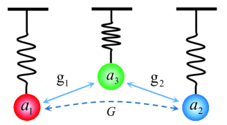
Figure 1: Schematic diagram for universal multimode interactions in a quantum system. Each mode can be represented by a harmonic oscillator. $a_{3}$ is a intermediate mode for connecting two others.

II Multimode interactions and adiabatic quantum control

We show the three-mode quantum system in Fig. 1. Two harmonic oscillators couple to each other via the intermediate one. The effective Hamiltonian of this system is given by

$$\hat{H}_{1}=\text{g}_{1}\hat{a}_{1}^{{\dagger}}\hat{a}_{3}+\text{g}_{2}\hat{a}_{2}^{{\dagger}}\hat{a}_{3}+\text{H.c.},$$ (1)

where $\hat{a}_{i}$$(\hat{a}^{{\dagger}}_{i})$ $(i=1,2,3)$ are the annihilation (creation) operators for the corresponding $i$-th mode with the frequency $\omega_{i}$, respectively. $\text{g}_{i}(t)$ is the effective coupling strength between the corresponding mode with the intermediate one. The Heisenberg equations of the system can be derived as

$$id\vec{v}(t)/dt=M(t)\vec{v}(t),$$ (2)

where the vector operator $\vec{v}(t)=[\hat{a}_{1}(t),\hat{a}_{3}(t),\hat{a}_{2}(t)]^{T}$, and the matrix $M(t)$ can be expressed as

$$M(t)=\left[\begin{array}[]{ccc}0&\text{g}_{1}(t)&0\\ \text{g}_{1}(t)&0&\text{g}_{2}(t)\\ 0&\text{g}_{2}(t)&0\\ \end{array}\right].$$ (6)

The matrix $M(t)$ has the eigenvalues $\lambda=0,\pm\text{g}_{0}$ and the corresponding eigenmodes are $\psi_{1}=[-\text{g}_{2}/\text{g}_{0},0,\text{g}_{1}/\text{g}_{0}]^{T}$ and $\psi_{2,3}=[\text{g}_{1}/\text{g}_{0},\pm 1,\text{g}_{2}/\text{g}_{0}]^{T}/\sqrt{2}$, where $\text{g}_{0}=\sqrt{\text{g}^{2}_{1}+\text{g}^{2}_{2}}$. The eigenmode $\psi_{1}$ with the eigenvalues $\lambda=0$ is a dark mode which decouples with the intermediate mode.

The adiabatic quantum control is a very effective approach for quantum information processing between the modes 1 and 2, such as the quantum state transfer between these two modes. It is robust against the dissipation from the intermediate mode by evolving along the dark state adiabatically. However, to suppress the undesired transition between different eigenmodes, the near perfect adiabatic process needs so long time that accumulates more decoherence in the whole process. This infidelity is a big challenge for an adiabatic quantum control.

III Fast and robust quantum control for multimode interactions

To improve the speed and mitigate the infidelity, we use the STA to speed up the adiabatic process in three-mode interactions of a quantum system. The main obstacle for accelerating the adiabatic process is the transition amplitude between eigenmodes which will increase when the speed is accelerated. If the speed is up, the evolution path will deviate the original way and more inherent errors are produced. Therefore, the robustness becomes lower. To overcome this mutual restriction, removing the transition is the first task. According to the TQD algorithm MVBerry2009 , we can find a new way with no undesired transitions and calculate the matrix $M_{1}(t)$ by using the formula (see appendix for more details) given by

$$M_{1}(t)=i\sum_{n}|\frac{\partial\psi_{n}(t)}{\partial t}\rangle\langle\psi_{n}(t)|,$$ (7)

where $|n(t)\rangle$ is the eigenmode. Substituting the all eigenmodes into Eq. (7), one can get a new matrix $M^{\prime}(t)$ given by

$$M_{1}(t)=i\sum_{n=1}^{3}\dot{\psi}_{n}\psi_{n}^{{\dagger}}=\left[\begin{array}[]{ccc}0&0&iG\\ 0&0&0\\ -iG&0&0\\ \end{array}\right],$$ (11)

where $G=(\dot{\text{g}}_{1}\text{g}_{2}-\text{g}_{1}\dot{\text{g}}_{2})/\text{g}^{2}_{0}$. The result of the matrix $M_{1}(t)$ indicates that there exists a direct transition between the modes 1 and 2. We choose the adiabatic coupling strengths with ‘Vitanov’ shape Vasilevpra given by

$$\text{g}_{1}(t)=\text{g}_{0}\sin(\theta(t)),$$

$$\text{g}_{2}(t)=\text{g}_{0}\cos(\theta(t)),$$

$$\theta(t)=\frac{\pi}{2}\frac{1}{1+e^{-\nu(t-5/\nu)}}.$$ (12)

Here, $\nu$ describes the duration of coupling strengths. Therefore, with above functions, the transitionless matrix $M_{1}$ is given by making $G=\dot{\theta}(t)$ in Eq.(11). The comparison between the adiabatic quantum control and the accelerated TQD protocol in quantum state transfer process is shown in Fig. 2. We change the duration of coupling strengths and the adiabatic processes are accelerated. But the results become imperfect. However, by using the TQD, the new quantum control processes always keep the perfect result in the population transfer. Comparing (g), (h) and (i) in Fig. 2, the final time for completing the quantum state transfer becomes shorter. The total time in Fig. 2 (i) is three times shorter than Fig. 2 (g).

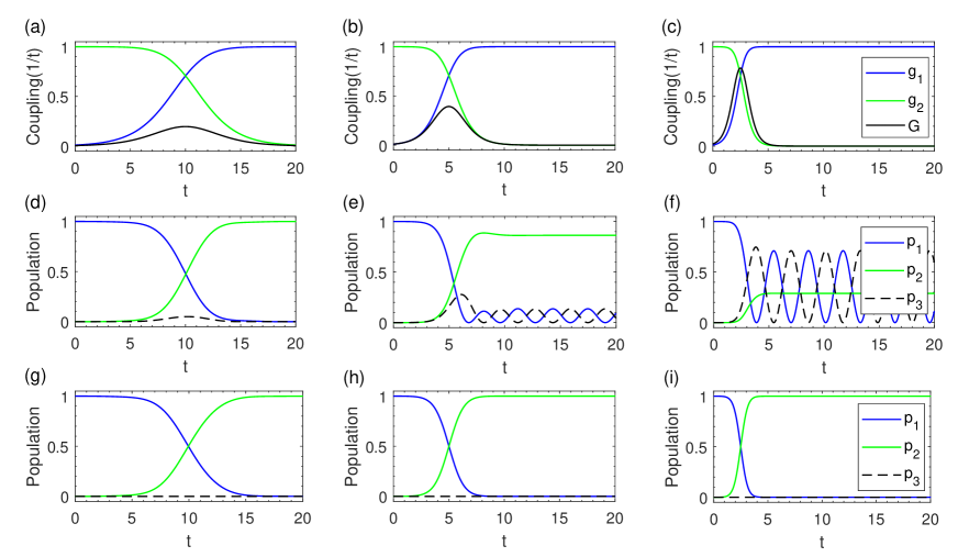
Figure 2: Simulation of two quantum control approaches for the quantum state transfer in multimode interactions. The initial state is prepared in mode $a_{1}$ with the Fock state $|1\rangle$. All the labels for curves with different colors are given in the last figures of every row. $\text{p}_{1}$, $\text{p}_{2}$ and $\text{p}_{3}$ are the populations for the modes $a_{1}$, $a_{2}$ and $a_{3}$, respectively. (a)-(c) are the variation of coupling strengths. (d)-(f) are the corresponding adiabatic quantum control processes. (g)-(i) are the corresponding fast and robust quantum control processes. The parameter changes as follow: (a) $\nu=0.5$ MHz; (b) $\nu=1$ MHz; (c) $\nu=2$ MHz.

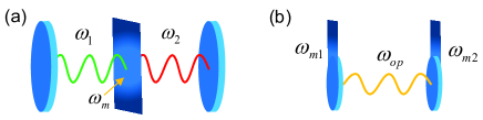
Figure 3: (a) Practical schematic diagram for photon-phonon-photon interactions induced by the optomechanical system composed of two cavities and a membrane. The two cavity walls and the middle membrane are fixed, but the membrane can vibrate. (b) Schematic diagram for phonon-phonon-phonon interactions. Two cavity walls are fixed on cantilevers.

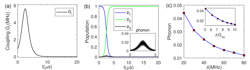
Figure 4: Simulation of the quantum state transfer by using our fast and robust quantum control in optomechanical interactions. (a) The shape of new coupling strengths with the parameters $\nu=2$ MHz and $\delta=40$ MHz. (b) The process of the population transfer by using the coupling in (a). $P_{1}$, $P_{2}$ and $P_{3}$ are the populations for the optical modes 1, 2 and the mechanical mode, respectively. The population of the phonon is amplified in the insert. (c) Variation of the maximal average phonon number with detuning. The insert is the variation of the maximal average phonon number vs the rate between detuning and the maximal coupling strength.

IV Practical application for photon-phonon interactions

A typical physical system for photon-phonon interactions is an optomechanical one. For three-mode interactions in this quantum system, there are two kinds of interactions, i.e., the photon-phonon-photon interaction shown in Fig. 3(a) and the phonon-photon-phonon interaction shown in Fig. 3(b). Here, we consider Fig. 3(a) in which an optomechanical system composed of two cavity modes coupled to each other via the mechanical mode. Two optical cavities connect to each other via a middle membrane. After the standard linearization procedure, the Hamiltonian of the system is given by ($\hbar=1$) LTianPRL2012 ; YDWangPRL2012

$$\hat{H}_{2}=\omega_{m}\hat{b}^{{\dagger}}\hat{b}+\!\!\!\sum_{i=1,2}\!\!\left[-\Delta_{i}\hat{a}^{{\dagger}}_{i}\hat{a}_{i}+G_{i}(\hat{a}^{{\dagger}}_{i}+\hat{a}_{i})(\hat{b}+\hat{b}^{{\dagger}})\right]\!,$$ (13)

where $\hat{a}_{i}$$(\hat{a}^{{\dagger}}_{i})$ $(i=1,2)$ and $\hat{b}$$(\hat{b}^{{\dagger}})$ are the annihilation (creation) operators for the $i$-th cavity mode with frequency $\omega_{i}$ and the mechanical mode, respectively. $\omega_{m}$ is the mechanical frequency. $\Delta_{i}=\omega_{di}-\omega_{i}$ and $G_{i}=G_{0i}\sqrt{n_{i}}$ are the laser detuning and the effective linear coupling strength, respectively. $G_{0i}$ and $n_{i}$ are the single-photon optomechanical coupling rate and the intracavity photon number induced by the driving field with the frequency $\omega_{di}$, respectively. We consider the case that both cavity modes are driven near the red sidebands. In the interaction picture, the Hamiltonian of the system becomes (under the rotating-wave approximation)

$$\hat{H}_{3}=\sum_{i=1,2}\delta_{i}\hat{a}_{i}^{{\dagger}}\hat{a}_{i}+G_{i}(\hat{a}_{i}^{{\dagger}}\hat{b}_{m}+\hat{b}_{m}^{{\dagger}}\hat{a}_{i}),$$ (14)

where $\delta_{i}=-\Delta_{i}-\omega_{m}$. The Heisenberg equation of the system can be derived with

$$id\vec{v}_{op}(t)/dt=M_{op}(t)\vec{v}_{op}(t),$$ (15)

where the vector operator $\vec{v}_{op}(t)=[\hat{a}_{1}(t),\hat{b}_{m}(t),\hat{a}_{2}(t)]^{T}$, and the matrix $M_{op}(t)$ is the same as Eq.(6) with the condition $\delta_{i}=0$. There exists an optomechanical dark mode CHDongscience and it is used to make the adiabatic control with quantum information processing between two optical modes.

To realize a fast and robust quantum control for above process, we usually need seek a direct coupling between two optical modes based on Eq.(11). Here, it is hard to construct a direct coupling and we replace it with an effective two-mode interaction. We set the large detuning condition with $\delta_{i}\gg G_{i}$ in Eq.(14) and the large energy offsets suppress the transitions between the optical mode and the mechanical mode JICiracPRL1997 ; HKLiPRA2013 . Hence, one can adiabatically eliminate the mechanical mode $\hat{b}$ and obtain the effective beam-splitter-like Hamiltonian

$$\hat{H}_{4}=\sum_{i=1,2}(\delta_{i}+\Omega_{i})\hat{a}_{i}^{{\dagger}}\hat{a}_{i}+\Omega(\hat{a}^{{\dagger}}_{1}\hat{a}_{2}+\hat{a}^{{\dagger}}_{2}\hat{a}_{1}),$$ (16)

where $\Omega_{i}=G^{2}_{i}/\delta_{i}$ and $\Omega=G_{1}G_{2}(\delta^{-1}_{1}+\delta^{-1}_{2})/2$. We set $\delta_{1}+\Omega_{1}=\delta_{2}+\Omega_{2}$ and $\delta=\delta_{1}=\delta_{2}$. In the new interaction picture under the Hamiltonian $\hat{H}_{0}=\sum_{i=1,2}(\delta_{i}+\Omega_{i})\hat{a}_{i}^{{\dagger}}\hat{a}_{i}$, one can derive the matrix $M_{2}(t)$ in the Heisenberg picture with

$$M_{2}(t)=\left[\begin{array}[]{ccc}0&0&\frac{G_{1}G_{2}}{\delta}\\ 0&0&0\\ \frac{G_{1}G_{2}}{\delta}&0&0\\ \end{array}\right].$$ (20)

The effective matrix $M_{2}(t)$ is equivalent to $M_{1}(t)$ shown in Eq. (7) derived by the TQD algorithm, when

$$\frac{G_{1}G_{2}}{\delta}=\frac{\text{g}_{1}\dot{\text{g}}_{2}-\dot{\text{g}}_{1}\text{g}_{2}}{\text{g}^{2}_{0}}.$$ (21)

The evolutions of the photon and the phonon in the system are plotted in Fig. 4 by using the Hamiltonian in Eq.(14). With the adiabatic coupling Eq.(III), Eq.(21) becomes $G_{1}G_{2}=\delta\dot{\theta}(t)$. Here, we design the coupling with $G_{1}=G_{2}$ shown in Fig. 4(a). The other parameters should be chosen to satisfy the large detuning condition $\delta^{\prime}\gg G_{i}$ and $\delta_{1}+\Omega_{1}=\delta_{2}+\Omega_{2}$. Here we choose $\delta=40$ MHz and $\nu=2$ MHz.

The photon in cavity 1 is transferred to cavity 2 by using our protocol with a higher fidelity, shown in Fig. 4(b). The phonon number is suppressed in the whole process and the maximum value is about 0.02 due to the large detuning interaction. From Fig. 4(c), one can see that the maximal average phonon number is inversely proportional to the rate between the detuning and the maximal coupling strength.

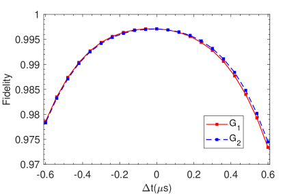
Figure 5: Fidelities for the parameter time deviation $\Delta t$. The range of the time interval is $[-0.60,0.60]$. The positive and negative values represent the time delay and advance, respectively. $G_{1}$ ($G_{2}$) is the result from changing $G_{1}$ ($G_{2}$) and keeping $G_{2}$ ($G_{1}$) unchanged. The parameters are chosen to be $\nu=2$ MHz and $\delta=40$ MHz.

V Analysis of robustness and fidelity

It is hard to accurately control the time interval between two coupling strengths in the actual experiment. Therefore we consider the influence caused by a small deviation of the time interval in Fig. 5. We tune the time interval from $-0.6\mu$s to $0.6\mu$s, and the results indicates that our protocol is insensitive to the deviation of the time interval.

When the dissipation of the mechanical oscillator and the decay of the cavity is taken into account, the dynamics of the quantum system described by the Lindblad form master equation is expressed by

$$\frac{d\hat{\rho}}{dt}=i[\hat{\rho},\hat{H}_{s}(t)]\!+\kappa_{1}\hat{L}[\hat{a}_{1}]\hat{\rho}\!+\kappa_{2}\hat{L}[\hat{a}_{2}]\hat{\rho}\!+\gamma_{m}\hat{D}[\hat{b}_{m}]\hat{\rho},\;\;\;\;$$ (22)

where $\hat{\rho}$ and $\hat{H}_{s}(t)$ are the density matrix and the Hamiltonian of the multimode interactions, respectively. $\kappa_{1}$ and $\kappa_{2}$ represent the decay rates of the cavities 1 and 2, respectively. $\gamma_{m}$ is the mechanical damping rate. $\hat{L}[\hat{A}]\hat{\rho}=(2\hat{A}\hat{\rho}\hat{A}^{{\dagger}}-\hat{A}^{{\dagger}}\hat{A}\hat{\rho}-\hat{\rho}\hat{A}^{{\dagger}}\hat{A})/2$. $\hat{D}[\hat{A}]\hat{\rho}=(n_{th}+1)(2\hat{A}\hat{\rho}\hat{A}^{{\dagger}}-\hat{A}^{{\dagger}}\hat{A}\hat{\rho}-\hat{\rho}\hat{A}^{{\dagger}}\hat{A})/2+n_{th}(2\hat{A}^{{\dagger}}\hat{\rho}\hat{A}-\hat{A}\hat{A}^{{\dagger}}\hat{\rho}-\hat{\rho}\hat{A}\hat{A}^{{\dagger}})/2$, where $n_{th}$ is the thermal phonon number of the environment. Here, we choose the Hamiltonian $\hat{H}_{3}$ to calculate the master equation. We choose the parameters $\gamma_{m}=500$ Hz and $n_{th}=100$ and change the decay $\kappa=\kappa_{1}=\kappa_{2}$. We calculate the fidelity with the formula $F=\langle 01|tr_{m}[\hat{\rho}(t)]|01\rangle$. Here $|01\rangle$ represents the state which there are zero and one photon in the cavities 1 and 2, respectively. $tr_{m}[\hat{\rho}(t)]$ is the reduced density matrix by tracing the mechanical oscillator degree of freedom. The fidelities are plotted in Fig. 6(a) and (b) for the adiabatic and fast protocols, respectively. The fidelities of the fast protocol are higher than the adiabatic protocol. As the process is accelerated, the total evolution time is shorter.

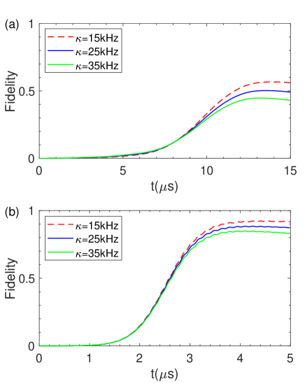
Figure 6: Fidelity of the TQD process in the present of different dissipations $\kappa$ in optomechanical interactions. (a) Fidelities for the adiabatic quantum control. Here, we choose $\nu=0.5$ MHz. (b) Fidelities for the fast quantum control process. Parameters are chosen as $\gamma_{m}=500$ Hz and $n_{th}=100$.

VI Conclusion

To conclude, we have proposed a universal protocol to realize a fast and robust quantum control for multimode interactions in a quantum system by using STA. We also have applied this protocol in a practical photon-phonon-photon interaction model for the quantum state transfer in quantum information processing. Our protocol has the following remarkable advantages. First, compared with the adiabatic protocol, it is faster as it can improve the speed of a multimode interaction, which reduces more decoherence in the whole evolution process of the quantum system. Second, under the fast process, there is no undesired transition between eigenmodes. Third, it is also robust to some practical experimental imperfections. These good features can effectively improve the feasibility of practical applications of multimode interactions in quantum information processing in experiment.

APPENDIX: TRANSITIONLESS QUANTUM DRIVING ALGORITHM FOR MULTIMODE INTERACTIONS

Let us consider a quantum system with an arbitrary time-dependent Hamiltonian $\hat{H}_{0}(t)$. The dynamical process is described by

$$\hat{H}_{0}(t)|n(t)\rangle=E_{n}(t)|n(t)\rangle,$$ (23)

where $|n(t)\rangle$ and $E_{n}(t)$ are the instantaneous eigenstate and the eigenenergies of $\hat{H}_{0}(t)$, respectively. According to the adiabatic approximation MBorn1928 , the dynamical evolution of states driven by $\hat{H}_{0}(t)$ could be expressed as

$$|\psi_{n}(t)\rangle\!\!=\!\exp\left\{\!-i\!\!\int^{t}_{0}\!\!\!dt^{\prime}E_{n}(t^{\prime})\!-\!\!\int^{t}_{0}\!\!\!dt^{\prime}\langle n(t^{\prime})|\dot{n}(t^{\prime})\rangle\right\}|n(t)\rangle,$$

where $|\psi_{n}(t)\rangle$ is the state of system at time $t$. Now, we seek a new Hamiltonian $\hat{H}(t)$ based on the reverse engineering approach to satisfy the Schrödinger equation

$$i|\dot{\psi}_{n}(t)\rangle=\hat{H}(t)|\psi_{n}(t)\rangle.$$ (25)

Any time-dependent unitary operator $\hat{U}(t)$ is also given by

$$i\dot{\hat{U}}(t)=\hat{H}(t)\hat{U}(t),$$ (26)

and

$$\hat{H}(t)=i\dot{\hat{U}}(t)\hat{U}^{{\dagger}}(t).$$ (27)

In order to guarantee no transitions between the eigenstates of $\hat{H}_{0}(t)$ for any time, the time-dependent unitary operator $\hat{U}(t)$ should have the form

$$\hat{U}(t)\! \!=\! \!\sum_{n}\exp\left\{-i\!\int^{t}_{0}\!\!dt^{\prime}E_{n}(t^{\prime})-\!\!\int^{t}_{0}\!\!dt^{\prime}\langle n(t^{\prime})|\dot{n}(t^{\prime})\rangle\right\}$$ (28)

$$\!\otimes|n(t)\rangle\langle n(0)|.$$

According to Eq. (27), the new Hamiltonian is given by

$$\hat{H}(t)\! \!=\! \!\sum_{n}|n\rangle E_{n}\langle n|+i\sum_{n}(|\dot{n}\rangle\langle n|-\langle n|\dot{n}\rangle|n\rangle\langle n|)$$ (29)

$$\!=\! \!\hat{H}_{0}(t)+\hat{H}_{cd}(t),$$

where $\hat{H}_{cd}(t)$ is the counter-diabatic Hamiltonian. The transitions of order $\exp(-1/\varepsilon)$ generated by $\hat{H}_{0}(t)$ can be eliminated by $\hat{H}_{cd}(t)$. One can find infinitely many Hamiltonians $\hat{H}(t)$ which differ from each other only by a phase. We disregard the phase factors ETorronteguiAAMOP2013 ; ACSantosPRA2016 and give the simplest Hamiltonian derived with MVBerry2009

$$\hat{H}(t)=i\sum_{n}|\dot{n}\rangle\langle n|.$$ (30)

Here $\hat{H}$ is the couterdiabatic term and purely non-diagonal in the basis $\{|n\rangle\}$.

In a three-mode quantum system, we should calculate a new matrix $M^{\prime}(t)$ which determines the evolution of Heisenberg equations with no undesired transition. First, we assume the time-dependent evolution operator for $M^{\prime}(t)$ which is given by

$$i\dot{\hat{U}}_{H}(t)=M^{\prime}(t)\hat{U}_{H}(t).$$ (31)

One can solve the $M^{\prime}(t)$ matrix via the equation given by

$$M^{\prime}(t) = i\left[\frac{\partial}{\partial t}\hat{U}_{H}(t)\right]\hat{U}_{H}^{{\dagger}}(t)$$ (32)

$$= i\sum_{n}|\frac{\partial\psi_{n}(t)}{\partial t}\rangle\langle\psi_{n}(t)|,$$

where $\hat{U}_{H}(t)=\sum_{n}|\psi_{n}(t)\rangle\langle\psi_{n}(0)|$. Here, $|\psi_{n}(t)\rangle$ is the eigenmode of the three-mode quantum system.

References

- (1) N. V. Vitanov, T. Halfmann, B. W. Shore, and K. Bergmann, Laser-induced population transfer by adiabatic passage techniques, Annu. Rev. Phys. Chem. 52, 763 (2001).
- (2) K. Bergmann, H. Theuer, and B. Shore, Coherent population transfer among quantum states of atoms and molecules, Rev. Mod. Phys. 70, 1003 (1998).
- (3) M. Born and V. Fock, Beweis des Adiabatensatzes, Z. Phys. 51, 165 (1928).
- (4) J. P. Davis and P. Pechukas, Nonadiabatic transitions induced by a time-dependent Hamiltonian in the semiclassical/adiabatic limit: the two-state case, J. Chem. Phys. 64, 3129 (1976).
- (5) J. T. Hwang and P. Pechukas, The adiabatic theorem in the complex plane and the semiclassical calculation of nonadiabatic transition amplitudes, J. Chem. Phys. 67, 4640 (1977).
- (6) E. Torrontegui, S. Ibáñez, S. Martínez-Garaot, M. Modugno, A. Campo, D. Guéry-Odelin, A. Ruschhaupt, X. Chen, and J. G. Muga, Shortcuts to adiabaticity, Adv. Atom. Mol. Opt. Phys. 62, 117 (2013).
- (7) H. R. Lewis and W. B. Riesenfeld, An exact quantum theory of the time-dependent harmonic oscillator and of a charged particle in a time-dependent electromagnetic field, J. Math. Phys. 10, 1458 (1969).
- (8) M. Demirplak and S. A. Rice, Adiabatic population transfer with control fields, J. Phys. Chem. A 107, 9937 (2003).
- (9) M. Demirplak and S. A. Rice, Assisted adiabatic passage revisited, J. Phys. Chem. B 109, 6838 (2005).
- (10) M. V. Berry, Transitionless quantum driving, J. Phys. A: Math. Theor. 42, 365303 (2009).
- (11) X. Chen, I. Lizuain, A. Ruschhaupt, D. Guéry-Odelin, and J. G. Muga, Shortcut to adiabatic passage in two- and three-Level atoms, Phys. Rev. Lett. 105, 123003 (2010).
- (12) X. Chen, E. Torrontegui, and J. G. Muga, Lewis-Riesenfeld invariants and transitionless quantum driving, Phys. Rev. A 83, 062116 (2011).
- (13) A. del Campo, Shortcuts to adiabaticity by counterdiabatic driving, Phys. Rev. Lett. 111, 100502 (2013).
- (14) S. Ibáñez, X. Chen, E. Torrontegui, J. G. Muga, and A. Ruschhaup, Multiple Schrödinger pictures and dynamics in shortcuts to adiabaticity, Phys. Rev. Lett. 109, 100403 (2012).
- (15) S. Martinez-Garaot, E. Torrontegui, X. Chen, and J. G. Muga, Shortcuts to adiabaticity in three-level systems using Lie transforms, Phys. Rev. A 89, 053408 (2014).
- (16) A. Baksic, H. Ribeiro, and A. A. Clerk, Speeding up adiabatic quantum state transfer by using dressed states, Phys. Rev. Lett. 116, 230503 (2016)
- (17) M. Lu, Y. Xia, L. T. Shen, and J. Song, An effective shortcut to adiabatic passage for fast quantum state transfer in a cavity quantum electronic dynamics system, Laser Phys. 24, 105201 (2014).
- (18) H. L. Mortensen, J. J. W. H. Sørensen, K. Mølmer, and J. F. Sherson, Fast state transfer in a -system: a shortcut-to-adiabaticity approach to robust and resource optimized control, New J. Phys. 20, 025009 (2018).
- (19) M. Lu, Y. Xia, L. T. Shen, J. Song, and N. B. An, Shortcuts to adiabatic passage for population transfer and maximum entanglement creation between two atoms in a cavity, Phys. Rev. A 89, 012326 (2014).
- (20) S. He, S. L. Su, D. Y. Wang, W. M. Sun, C. H. Bai, A. D. Zhu, H. F. Wang, and S. Zhang, Efficient shortcuts to adiabatic passage for three-dimensional entanglement generation via transitionless quantum driving, Sci. Rep. 6, 30929 (2016).
- (21) A. C. Santos and M. S. Sarandy, Superadiabatic controlled evolutions and universal quantum computation, Sci. Rep. 5, 15775 (2015).
- (22) Y. Liang, Q. C. Wu, S. L. Su, X. Ji, and S. Zhang, Shortcuts to adiabatic passage for multiqubit controlled-phase gate, Phys. Rev. A 91, 032304 (2015).
- (23) A. C. Santos, R. D. Silva, and M. S. Sarandy, Shortcut to adiabatic gate teleportation, Phys. Rev. A 93, 012311 (2016).
- (24) X. K. Song, H. Zhang, Q. Ai, J. Qiu, and F. G. Deng, Shortcuts to adiabatic holonomic quantum computation in decoherence-free subspace with transitionless quantum driving algorithm, New J. Phys. 18, 023001 (2016).
- (25) Y. H. Kang, Y. H. Chen, Q. C. Wu, B. H. Huang, Y. Xia, and J. Song, Reverse engineering of a Hamiltonian by designing the evolution operators, Sci. Rep. 6, 30151 (2016).
- (26) X. K. Song, Q. Ai, J. Qiu, and F. G. Deng, Physically feasible three-level transitionless quantum driving with multiple Schrödinger dynamics, Phys. Rev. A 93, 052324 (2016).
- (27) J. L. Wu, X. Ji, and S. Zhang, Shortcut to adiabatic passage in a three-level system via a chosen path and its application in a complicated system, Opt. Exp. 25, 21084-21093 (2017).
- (28) M. G. Bason, M. Viteau, N. Malossi, P. Huillery, E. Arimondo, D. Ciampini, R. Fazio, V. Giovannetti, R. Mannella, and O. Morsch, High-fidelity quantum driving, Nat. Phys. 8, 147–152 (2012).
- (29) Y. X. Du, Z. T. Liang, Y. C. Li, X. X. Yue, Q. X. Lv, W. Huang, X. Chen, H. Yan, and S. L. Zhu, Experimental realization of stimulated Raman shortcut-to-adiabatic passage with cold atoms, Nat. Commun. 7, 12479 (2016).
- (30) S. An, D. Lv, A. Campo, and K. Kim, Shortcuts to adiabaticity by counterdiabatic driving for trapped-ion displacement in phase space, Nat. Commun. 7, 12999 (2016).
- (31) J. Zhang, J. H. Shim, I. Niemeyer, T. Taniguchi, T. Teraji, H. Abe, S. Onoda, T. Yamamoto, T. Ohshima, J. Isoya, and D. Suter, Experimental implementation of assisted quantum adiabatic passage in a single spin, Phys. Rev. Lett. 110, 240501 (2013).
- (32) B. B. Zhou, A. Baksic, H. Ribeiro, C. G. Yale, F. J. Heremans, P. C. Jerger, A. Auer, G. Burkard, A. A. Clerk, and D. D. Awschalom, Accelerated quantum control using superadiabatic dynamics in a solid-state lambda system, Nat. Phys. 13, 330–334 (2017).
- (33) M. Aspelmeyer, T. J. Kippenberg, and F. Marquardt, Cavity optomechanics, Rev. Mod. Phys. 86, 1391 (2014).
- (34) M. Gao, F. C. Lei, C. G. Du, and G. L. Long, Self-sustained oscillation and dynamical multistability of optomechanical systems in the extremely-large-amplitude regime, Phys. Rev. A 91, 013833 (2015).
- (35) F. C. Lei, M. Gao, C. G. Du, Q. L. Jing, and G. L. Long, Three-pathway electromagnetically induced transparency in coupled-cavity optomechanical system, Opt. Express 23, 11508–11517 (2015).
- (36) X. Jiang, M. Wang, M. C. Kuzyk, T. Oo, G. L. Long, and H. Wang, Chip-based silica microspheres for cavity optomechanics, Opt. Express 23, 27260–27265 (2015).
- (37) C. Dong, V. Fiore, M. C. Kuzyk, and H. Wang, Optomechanical dark mode, Science 338, 1609–1613 (2012).
- (38) Y. D. Wang and A. A. Clerk, Using interference for high fidelity quantum state transfer in optomechanics, Phys. Rev. Lett. 108, 153603 (2012).
- (39) L. Tian, Adiabatic state conversion and pulse transmission in optomechanical systems, Phys. Rev. Lett. 108, 153604 (2012).
- (40) L. Tian, Robust photon entanglement via quantum interference in optomechanical interfaces, Phys. Rev. Lett. 110, 233602 (2013).
- (41) Y. D. Wang and A. A. Clerk, Reservoir-engineered entanglement in optomechanical systems, Phys. Rev. Lett. 110, 253601 (2013).
- (42) Q. Lin, J. Rosenberg, D. Chang, R. Camacho, M. Eichenfield, K. J. Vahala, and O. Painter, Coherent mixing of mechanical excitations in nano-optomechanical structures, Nat. Photon. 4, 236 (2010).
- (43) F. Massel, S. U. Cho, J.-M. Pirkkalainen, P. J. Hakonen, T. T. Heikkilä, and M. A. Sillanpää, Multimode circuit optomechanics near the quantum limit, Nat. Commun. 3, 987 (2012).
- (44) N. Spethmann, J. Kohler, S. Schreppler, L. Buchmann, and D. M. Stamper-Kurn, Cavity-mediated coupling of mechanical oscillators limited by quantum back-action, Nat. Phys. 12, 27 (2016).
- (45) M. C. Kuzyk and H. Wang, Controlling multimode optomechanical interactions via interference, Phys. Rev. A 96, 023860 (2017).
- (46) G. Vasilev, A. Kuhn, and N. Vitanov, Optimum pulse shapes for stimulated Raman adiabatic passage, Phys. Rev. A 80, 013417 (2009).
- (47) J. I. Cirac, P. Zoller, H. J. Kimble, and H. Mabuchi, Quantum state transfer and entanglement distribution among distant nodes in a quantum network, Phys. Rev. Lett. 78, 3221 (1997).
- (48) H. K. Li, X. X. Ren, Y. C. Liu, and Y. F. Xiao, Photon-photon interactions in a largely detuned optomechanical cavity, Phys. Rev. A 88, 053850 (2013).