A new method to probe the boundary where KAM tori persist by square matrix

Abstract

The nonlinear dynamics of a system can be analyzed using a square matrix. If off resonance, the lead vector of a Jordan chain in a left eigenspace of the square matrix is an accurate action-angle variable for sufficiently high power order. The deviation from constancy of the action-angle variable provides a measure of the stability of a trajectory. However, near resonance or the stability boundary, the fluctuation increases rapidly and the lead vector no longer represents an accurate action-angle variable. In this paper we show that near resonance or stability boundary, it is possible to find a set of linear combinations of the vectors in the degenerate Jordan chains as the action-angle variables by an iteration procedure so that the fluctuation is minimized. Using the Henon-Heiles problem as an example on resonance, we show that when compared with conventional canonical perturbation theory, the iteration leads to result in much more close agreement with the forward integration, and the iteration is convergent even very close to the stability boundary. It is further shown that the action-angle variables found in the iteration can be used to find another action-angle variables even much more closer to rigid rotations (KAM invariants). The fast convergent result is not in the form of polynomials, it is an exponential function with a rational function in the exponent more similar to a Laurent series than a Taylor series. Hence the method provides a new way to probe the boundary of the region where KAM tori exist.

The field of nonlinear dynamics has very wide area of application in sciencelieberman . In general, the more common approach is the forward numerical integration. To gain understanding, however, one prefers an approximate analytical solution to extract relevant information. “Integrable systems in their phase space contain lots of invariant tori and KAM Theory establishes persistence of such tori, which carry quasi-periodic motions” in small perturbationsbroer ; porshel ; arnold (4, 5). But the theory does not provide the stability boundary. An important issue is to find approximation to such KAM tori wherever they exist. Among the many approaches to this issue we may mention canonical perturbation theory, Lie algebra, power series, normal formlieberman ; Gustavson (6, 7, 8, 9, 10, 11, 12), etc. The results are often expressed as polynomials. However, for increased perturbation, near resonance, or for large amplitude, the solution of these perturbative approaches often lost precision.

The square matrix analysis developed recently nash (13, 14) has a potential in exploring these area. In the following sections, we first introduce the nonlinear dynamics square matrix equation, using the Henon-Heiles problemGustavson (6, 15) as an example. Then, in Section 2, we show that when off resonance the lead vector of the left Jordan chain is an approximate action-angle variable, and the expression derived for the frequency shift is a rational function rather than a polynomial. But on resonance, there are degenerate Jordan chains, the action-angle variables are no longer the lead vectors in the Jordan chains, they become the linear combinations of these vectors. In Section 2 we show for small amplitude a differential equation approach leads to an approximate solution, i.e., the approximate action-angle variables. Expressed in these variables the exact solution nearly represents rigid rotations but has amplitude and phase fluctuation. As the amplitude increases the fluctuation increases, and the approximation lost precision.

In Section 3, we show that for a given approximate solution, we can apply KAM theorem and use Fourier transform to find the coefficients of the linear combinations to minimize the fluctuation. In Section 4, we show that when the fluctuation is small, we can write the equations of motion in an exact form in terms of the action-angle variables and treat the fluctuation as a perturbation to the rigid rotations which serves as the zeroth order approximation. Then, in Section 5 we apply Fourier transform to solve this perturbation problem, and find the first order approximation. In Section 6, we show that the steps developed in section 3-5 form an iteration procedure. In each iteration step, we solve a set of linear equations to improve the the precision. Then, we use the Henon-Heiles problem as a numerical example to compare the iteration result with the canonical perturbation approach Gustavson (6). Finally, in Section 7, we show that the action-angle variables obtained by the iteration procedure, already in very close agreement with forward integration, can be used immediately to find another set of action-angle variables even much more closer to rigid rotations.

We summarize the result in the Conclusion: the numerical study shows that when the iteration procedure is convergent, it leads to accurate solution for a rather general type of nonlinear dynamics problem, the convergence region provides information about the boundary where KAM tori persist, and, since the perturbation is determined by the ratio of fluctuation over the amplitude rather than amplitude itself, it is different from, or might be even beyond the conventional canonical perturbation theory.

Our goal is to find the boundary where the KAM tori persist. The numerical study suggests the border of the convergence region of the iteration is very close to this boundary. However, our knowledge about the convergence so far is limited to numerical study of the Henon-Heiles problem. The relation between the convergence and the chaotic boundary is still unknown, and an analytical analysis of this relation would be a very important open issue.

1 Introduction: square matrix equation for nonlinear dynamics

We consider the equations of motion of a nonlinear dynamic system, it can be expressed by a square matrix. We use the Henon-Heiles problem Gustavson (6, 15) as an example, the Hamiltonian and the equations of motion are

$$H=\frac{1}{2}(x^{2}+p_{x}^{2}+y^{2}+p_{y}^{2})+x^{2}y-\frac{1}{3}y^{3}$$

$$\dot{x}=p_{x}$$

$$\dot{y}=p_{y}$$ (1.1)

$$\dot{p}_{x}=-x-2xy$$

$$\dot{p}_{y}=-y-x^{2}+y^{2}$$

If we use the complex variables $z_{x}\equiv x-ip_{x},\,z_{x}^{*}\equiv x+ip_{x},z_{y}\equiv y-ip_{y},z_{y}^{*}\equiv y+ip_{y}$ to form a row of monomials $Z^{T}$$\equiv$ $\{z_{x},z_{x}^{*}$, $z_{y},z_{y}^{*},$ $z_{x}^{2},z_{x}z_{x}^{*},z_{x}z_{y}$, $z_{x}z_{y}^{*},z_{x}^{*2}$, $z_{x}^{*}z_{y}$,$z_{x}^{*}z_{y}^{*}$, $z_{y}^{2}$,$z_{y}z_{y}^{*}$, $z_{y}^{*2}$,$z_{x}^{3}$, $z_{x}^{2}z_{x}^{*}$, $...$, $z_{y}^{*3}\}$, we can write the following equations for the derivatives of the column $Z$

$$\dot{z}_{x}=iz_{x}+\frac{i}{2}z_{x}z_{y}+\frac{i}{2}z_{x}^{*}z_{y}+\frac{i}{2}z_{x}z_{y}^{*}+\frac{i}{2}z_{x}^{*}z_{y}^{*}$$

$$\dot{z}_{x}^{*}=-iz_{x}^{*}-\frac{i}{2}z_{x}z_{y}-\frac{i}{2}z_{x}^{*}z_{y}-\frac{i}{2}z_{x}z_{y}^{*}-\frac{i}{2}z_{x}^{*}z_{y}^{*}$$

$$\dot{z}_{y}=iz_{y}+\frac{i}{4}z_{x}^{2}+\frac{i}{2}z_{x}z_{x}^{*}+\frac{i}{4}z_{x}^{*2}-\frac{i}{4}z_{y}^{2}-\frac{i}{2}z_{y}z_{y}^{*}-\frac{i}{4}z_{y}^{*2}$$

$$\dot{z}_{y}^{*}=-iz_{y}^{*}-\frac{i}{4}z_{x}^{2}-\frac{i}{2}z_{x}z_{x}^{*}-\frac{i}{4}z_{x}^{*2}+\frac{i}{4}z_{y}^{2}+\frac{i}{2}z_{y}z_{y}^{*}+\frac{i}{4}z_{y}^{*2}$$ (1.2)

$$\frac{d}{dt}z_{x}^{2}=2z_{x}\dot{z}_{x}=2iz_{x}^{2}+iz_{x}^{2}z_{y}+iz_{x}z_{x}^{*}z_{y}+iz_{x}^{2}z_{y}^{*}+iz_{x}z_{x}^{*}z_{y}^{*}$$

$$\frac{d}{dt}(z_{x}z_{x}^{*})=\frac{i}{2}z_{x}^{*2}z_{y}-\frac{i}{2}z_{x}^{2}z_{y}+\frac{i}{2}z_{x}^{*2}z_{y}^{*}-\frac{i}{2}z_{x}^{2}z_{y}^{*}$$

$$....$$

$$\frac{d}{dt}z_{y}^{*3}=3z_{y}^{*2}\dot{z}_{y}^{*}=-3iz_{y}^{*3}$$

As an example, we only keep the monomials to a power order of $n_{s}=3$. The monomials are ordered according to power order from low to high. Within each power order $n_{k}$, arrange the monomials so the first variable power starts from power $n_{m}=n_{k}$ and followed by decreasing power. For those terms with the first factor as monomial $z_{x}^{n_{m}}$, other variables are arranged according to the same rule for a sequence with power order $n_{k}-n_{m}$. One can show that the number of terms of power order $n_{k}$ is $(n_{k}+1)(n_{k}+2)(n_{k}+3)/6$, so for power $n_{k}=1,2,3$ the numbers are 4,10,20 respectively. The total number of terms up to power $n_{s}$ is $4+10+20=(n_{s}+1)(n_{s}+2)(n_{s}+3)(n_{s}+4)/24-1=34$. Then the differential equations Eq.(1.1) can be represented approximately by a large $34\times 34$ square matrix $M$ as $\dot{{Z}}=MZ.$

The square matrix $M$ is upper-triangular, and has the following form with the dimension of its sub-matrices determined by the number of terms for each power order 4,10,20:

$$M=\begin{bmatrix}M_{11}&M_{12}&M_{13}\\ 0&M_{22}&M_{23}\\ 0&0&M_{33}\end{bmatrix}$$ (1.3)

The diagonal blocks $M_{11}$, $M_{22}$, $M_{33}$ are all diagonal matrices with dimension $4\times 4$, $10\times 10$, $20\times 20$ respectively, thus $M$ is a $34\times 34$ upper-triangular matrix. The diagonal elements of $M_{11}$, $M_{22}$, $M_{33}$ are $\{i,-i,i,-i\}$, $\{2i,0,2i,0,-2i,0,-2i,2i,0,-2i\}$,$\{3i,i,3i,...,-3i\}$, respectively. For the sake of space, we only give a part of the list. But one can recognize the pattern for the diagonal elements. If we only keep the linear terms in the first 4 rows of Eq.(1.2), and denote the eigenvalues of the linear part of the equations for $z_{x}$ and $z_{y}$ as $i\mu_{x}$ and $i\mu_{y}$ respectively, then $\mu_{x}=\mu_{y}\equiv\mu=1$, the system is on resonance. The solution would be $z_{x}=z_{y}=e^{i\mu t},z_{x}^{*}=z_{y}^{*}=e^{-i\mu t}$. This is the small amplitude limit of the solution. If we substitute these into $Z$, then $\dot{Z}(t=0)$ gives the diagonal elements.

The dimension of the off-diagonal blocks $M_{12}$, $M_{13}$, $M_{23}$ are $4\times 10$, $4\times 20$, $10\times 20$ respectively. Since there are no third power terms in the first 4 rows of Eq.(1.2) , $M_{13}=0$.

$$\begin{split}&M_{12}=\begin{bmatrix}0&0&\frac{i}{2}&\frac{i}{2}&0&\frac{i}{2}&\frac{i}{2}&0&0&0\\ 0&0&-\frac{i}{2}&-\frac{i}{2}&0&-\frac{i}{2}&-\frac{i}{2}&0&0&0\\ \frac{i}{4}&\frac{i}{2}&0&0&\frac{i}{4}&0&0&-\frac{i}{4}&-\frac{i}{2}&-\frac{i}{4}\\ -\frac{i}{4}&-\frac{i}{2}&0&0&-\frac{i}{4}&0&0&\frac{i}{4}&\frac{i}{2}&\frac{i}{4}\end{bmatrix},\ M_{23}=\\ &\setcounter{MaxMatrixCols}{20}\begin{bmatrix}0&0&i&i&0&i&i&0&0&0&0&0&0&0&0&0&0&0&0&0\\ 0&0&-\frac{i}{2}&-\frac{i}{2}&0&0&0&0&0&0&0&\frac{i}{2}&\frac{i}{2}&0&0&0&0&0&0&0\\ ...&...&...&...&...&...&...&...&...&...&...&...&...&...&...&...&...&...&...&...\\ 0&0&0&-\frac{i}{2}&0&0&-i&0&0&0&0&0&-\frac{i}{2}&0&0&0&0&\frac{i}{2}&i&\frac{i}{2}\end{bmatrix}\end{split}$$ (1.4)

The dimension of $M$ increases rapidly with the power order $n_{s}.$ However, because $M$ is upper-triangular, it is straight forward to find its Jordan subspaces with much lower dimensions, and the eigenvalues of these eigenspaces are the diagonal elements. For example, for $n_{s}=5$, $M$ is a $125\times 125$ matrix. The lengths of the Jordan chains are 3, 2, 1yu (14). Each chain forms the basis of an invariant subspace. Only for the longest chains with eigenvalue $i\mu_{x}$ or $i\mu_{y}$, the lead vector has all the monomials from linear terms to power $n_{s}$. For all other chains, the lead vectors have only higher power terms. Hence our study is focused on these longest chains. In general, the Jordan chains are not uniquely defined. However there is a way to define them uniquely so the lead vector for each chain with those terms of form $z_{x}(z_{x}z_{x}^{\ast})^{m_{x}}(z_{y}z_{y}^{\ast})^{m_{y}}$, or $z_{y}(z_{x}z_{x}^{\ast})^{m_{x}}(z_{y}z_{y}^{\ast})^{m_{y}}$, i.e., the terms of form of $z_{x}$,$z_{y}$ times an invariant monomial removed(see in Appendix E of yu (14)). For Henon-Heiles problem, the system is on resonance with $\mu_{x}=\mu_{y}=1$, so if $n_{s}=5$, the two invariant subspace formed by the two longest chains with the eigenvalue $i\mu_{x}$ and $i\mu_{y}$ joined into one invariant subspace of dimension 6, much lower than the dimension of $M$.

2 The Action Angle Variables based on Jordan Decomposition of Square matrix

For a square matrix equation $\dot{Z}=MZ$ as discussed in yu (14), for one Jordan chain $U$ in the left eigenspace of $M$, we have

$$\begin{split}&UM=NU\\ &\frac{d(UZ)}{dt}=U\dot{Z}=UMZ=NUZ\end{split}$$ (2.1)

where $U$ is a rectangular matrix with each row a left eigenvector in the Jordan chain, arranged in the order of the chain so the first row is its lead vector. $N\equiv i\mu+\tau$ is the Jordan form in one of the Jordan blocks we are interested in, i.e., the chain of generalized eigenvectors of $M$ with eigenvalue $i\mu$. Now introduce $W\equiv UZ$, with

$$W=\begin{bmatrix}\,w_{0}\\ \,w_{1}\\ \,w_{2}\\ ...\end{bmatrix}\text{{\ and\ }}\tau W=\begin{bmatrix}0&1&0&...&0\\ 0&0&1&...&0\\ 0&0&...&...&0\\ 0&0&0&...&1\\ 0&0&0&...&0\end{bmatrix}\begin{bmatrix}\,w_{0}\\ \,w_{1}\\ \,w_{2}\\ ...\end{bmatrix}=\begin{bmatrix}\,w_{1}\\ \,w_{2}\\ ...\\ \,0\end{bmatrix}$$ (2.2)

where $w_{0}=u_{0}Z,\,w_{1}=u_{1}Z,\ldots$ are the projection of vector $Z$ onto the eigenvectors $u_{0},\,u_{1},\ldots$(the rows of $U$). During the motion, $Z$ rotates in the space of all polynomials within a given power order $n_{s}$. Hence the vectors $w_{0},\,w_{1},\,\ldots$ also rotate in the subspace with eigenvalue $i\mu$. From Eq.(2.1), we have

$$\begin{split}&\dot{W}=(i\mu+\tau)W\end{split}$$ (2.3)

When far away from resonances, $W$ is approximately an eigenvector of $\tau$. That is, it is a “coherent” state glauber (16, 17) with eigenvalue $i\phi$, as discussed in yu (14). $\phi$ is nearly a constant representing the amplitude dependent frequency shift from the zero amplitude frequency $\mu$. For this case, in Eq.(2.3) $\tau$ is approximately replaced by $i\phi$: $\dot{w}_{0}\approx i(\mu+\phi)w_{0},\dot{w}_{1}$ $\approx i(\mu+\phi)w_{1},\cdots$, with $\phi\approx w_{1}/w_{0}\approx w_{1}/w_{2}\approx\cdots$. Hence the frequency shift $\phi$ is a rational function rather than a polynomial. Each row of $W$ in Eq.(2.2) is an approximation of the action-angle variable. The lead vector $w_{0}$ has terms from linear to high power terms, $w_{1}$ has only terms of power higher than 2, while all other $w_{j}$ with $j>1$ has only terms of power higher than 4. Hence we can write $v\equiv re^{i\theta}\approx w_{0}$ as the action-angle variable approximation while all other $w_{j}$s are less acurate action-angle variables with only higher power terms.

For the case of two variables $x$ and $y$, we consider two eigenspaces and find the Jordan chain $W_{x}$ $\{w_{x0}=u_{x0}Z,$ $w_{x1}=u_{x1}Z,\ldots$} , and Jordan chain $W_{y}$ {$w_{y0}=u_{y0}Z,\,w_{y1}=u_{y1}Z,\ldots$ }, with eigenvalues $i\mu_{x,}i\mu_{y}$ respectively. Similarly we find two independent action-angle variable approximations $v_{x}\equiv r_{x}e^{i\theta_{x}}\approx w_{x0}$, $v_{y}\equiv r_{y}e^{i\theta_{y}}\approx w_{y0}$. The rotations of these two vectors form two independent rigid rotations with approximately constant phase advance rates $\dot{\theta}_{x}=\mu_{x}+\phi_{x}$ and $\dot{\theta}_{y}=\mu_{y}+\phi_{y}$ respectively. As described in yu (14), these variables provide excellent solution to the nonlinear dynamics problem when off resonances.

However, when on resonance, $\mu_{x}=\mu_{y}=\mu$, the two blocks $W_{x}$ and $W_{y}$ are degenerate. They are no longer approximate eigenvectors of $\tau$. In spite of this, because the projection of the trajectory $Z$ onto the eigenspace $\mu$ must remain in this invariant subspace, it must be a linear combination of $w_{x0}$ ,$w_{y0}$, $w_{x1}$, and $w_{y1}\ldots$. In addition, KAM theory states that under small perturbation there must be a region around the fixed point where the invariant tori are stable, hence the corresponding linear combinations must have well defined frequencies, or, form a coherent state.

In the following, when we refer to the linear combinations, it is equivalent that we refer to the approximate action-angle variables. Thus the main issue in finding the solution becomes finding the coefficients of such linear combinations for which the corresponding action-angle variables evolve in a way that the deviation (i.e., the fluctuation) from rigid rotations is minimized. Thus, for each pair of approximate action-angle variables we associate it with an approximate trajectory, and a pair of rigid rotations. The deviation of the trajectory from the rigid rotations is to be minimized.

For the case on resonance in the Henon-Heiles problem of two variables $x$ and $y$, we are searching for two sets of linear combinations for two approximate action-angle variables as the solution. In the search for the linear combinations of the vectors in the eigenspace, we first consider the case of small amplitude. We neglect $w_{x1},w_{y1}\ldots$ , which only have high power terms. The vectors $w_{x1},w_{y1}\ldots$ have no linear terms, their contribution becomes important only for motion with large amplitude, as we shall describe later. Thus we look for coefficients in the linear combination $v\equiv a_{1}w_{x0}+a_{2}w_{y0}\text{ }$ such that $v=re^{i\omega t}$, where $r$ and $\omega$ are constant. Thus $v$ , as an approximate action-angle variable (in the following, to be brief, we abbreviate it as “action”), satisfies the equations

$$\begin{split}&\dot{v}=i\omega v\text{ }\\ &\ddot{{v}}=i\omega\dot{{v}}\end{split}\text{ }\hskip 28.45274pt$$ (2.4)

To derive an equation for $a_{1},a_{2}$, we substitute $v\equiv a_{1}w_{x0}+a_{2}w_{y0}\text{ }$ into Eq.(2.4). To calculate the derivatives, write Eq.(2.3) in an explicit matrix form, using the property of the Jordan matrix $\tau$, we found $\dot{w}_{0}=i\mu\,w_{0}+w_{1}$and $\ddot{w}_{0}=(i\mu)^{2}w_{0}+2i\mu\,w_{1}+w_{2}$. Applying these to the two degenerate chains $W_{x}$ and $W_{y}$ respectively, we get

$$\dot{v}=(i\mu\,w_{x0}+w_{x1})a_{1}+(i\mu\,w_{y0}+w_{y1})a_{2}$$

$$\ddot{v}=((i\mu)^{2}w_{x0}+2i\mu\,w_{x1}+w_{x2})a_{1}$$ (2.5)

$$\qquad+((i\mu)^{2}w_{y0}+2i\mu\,w_{y1}+w_{y2})a_{2}$$

Substitute each row of Eq.(2.5) into Eq.(2.4), let $i\phi=i\omega-i\mu$, we obtain an eigenequation

$$\begin{split}\begin{bmatrix}w_{x0}&w_{y0}\\ w_{x1}&w_{y1}\end{bmatrix}^{-1}\begin{bmatrix}w_{x1}&w_{y1}\\ w_{x2}&w_{y2}\end{bmatrix}A=i\phi A\end{split}\text{ }{\thinspace with\thinspace}\text{ }\hskip 2.84526ptA\equiv\begin{bmatrix}a_{1}\\ a_{2}\end{bmatrix}$$ (2.6)

This is a generalization of the off-resonance frequency shift $i\phi=\frac{w_{1}}{w_{0}}$. Now it is an eigenequation with two eigenvalues $\phi_{1}\equiv\omega_{1}-\mu$, $\phi_{2}\equiv\omega_{2}-\mu$. $w_{x0}$,$w_{y0}$,$w_{x1}$,$w_{y1}$,$w_{x2}$,$w_{y2}$ are polynomials of $x$,$p_{x}$,$y$,$p_{y}$. For a set of initial values $x_{0}$,$p_{x0}$,$y_{0}$,$p_{y0}$, Eq.(2.6) has two eigenvectors $A_{1},A_{2}$, which give the two sets of coefficients $\{a_{11},a_{12}\}$,$\{a_{21},a_{22}\}$ in $v\equiv a_{1}w_{x0}+a_{2}w_{y0}\text{ }$, corresponding to the two functions $v_{1}\equiv r_{1}e^{i\theta_{1}}$,$v_{2}\equiv r_{2}e^{i\theta_{2}}$. For small amplitude, they are excellent first order approximation of the action-angle variables. Thus $\theta_{1}\approx\omega_{1}t+\theta_{10}=(\mu+\phi_{1})t+\theta_{10}$ and $\theta_{2}\approx\omega_{2}t+\theta_{20}=(\mu+\phi_{2})t+\theta_{20}$ represent two independent rigid rotations, as required by KAM theorem. For small amplitude, the linear combination coefficients $a_{1},a_{2}$ are determined from the initial condition, and the deviation from the rigid rotations is negligibly small.

3 Calculation of Linear Combinations for Action-Angle Variables using a known trajectory

In the case of increased amplitude, the linear combination coefficients can no longer be determined by the initial value $x_{0}$,$p_{x0}$,$y_{0}$,$p_{y0}$ as in Eq.(2.6) but by $x$,$p_{x}$,$y$,$p_{y}$ in a larger neighborhood near the fixed point. The high power terms in Eq.(2.1), which are truncated in the construction of the square matrix in Eq.(2.3), serve as a perturbation to the rigid rotations as described in Poincare-Birkhoff theorem brown (12). Thus the main issue in finding the solution now becomes finding the coefficients of the linear combinations for large amplitude in a perturbation theory .

In the following we shall first show that if we have a numerical forward integration of the dynamic equations, i.e., if we have the trajectory, we can apply KAM theory and use Fourier expansion to determine the linear combinations that approximate rigid rotations. However, since our goal is to find the solution without the forward integration, later we shall not use the trajectory given by the forward integration. Instead, we use an approximate trajectory to determine the linear combinations approximately. The first approximate trajectory itself can be obtained by the method outlined in the Section 2, with the rigid rotation calculated from the linear combinations given by Eq.(2.6). The trajectory is going to be improved by an iteration procedure given in later sections.

KAM theory states that broer ; porshel under small perturbation there must be a domain (a Cantor set with positive measure) around the fixed point where the invariant tori (the perturbed rotation) are stable, and represent quasi-periodic motions. But the theory does not tell where the region is extended to. Our goal is to probe the boundary of this region. Within this boundary, according to Arnold’s theoremarnold (4), there is a variable transformation from the perturbed rotation to rigid rotation (see detailed explanation in wayne (5), where the perturbed rotation is referred to as being conjugated to the rigid rotation by the variable transform). In our notation, there exists a transformation from the trajectory $x,p_{x},y,p_{y}$ to the rigid rotation $v_{1}(x,p_{x},y,p_{y})=r_{1}e^{i\omega_{1}t},$ $v_{2}(x,p_{x},y,p_{y})=r_{2}e^{i\omega_{2}t}$, i.e., the action-angle variables. As an inverse function, the coordinates $x$,$p_{x}$,$y$,$p_{y}$ are the functions of $\theta_{1}\equiv\omega_{1}t$, $\theta_{2}\equiv\omega_{2}t$ (modulo $2\pi$), hence the eigenvectors $w_{x0}$ ,$w_{y0}$, $w_{x1}$, $w_{y1}\ldots$ can also be expanded in terms of $\theta_{1}$, $\theta_{2}$. This property of a trajectory as a function of $t$ can be represented by a periodic function of $\theta_{1}$, $\theta_{2}$ is critically important, so in the following search for approximate solutions, we limit them to periodic functions of $\theta_{1}$, $\theta_{2}$ (modulo $2\pi$) only. Our goal is to not only find the solution near the stability boundary, but more importantly, transform it into a specific form of rigid rotation using this property.

For simplicity in writing, if we choose $n_{v}$ eigenvectors for the linear combinations, we label them as $w_{j}$ with $j=1,2,..,n_{v}$. For example, for Eq.(2.4), $n_{v}=2$, $w_{1}\equiv w_{x0},w_{2}\equiv w_{y0}$. We have the expansion

$$w_{j}(\theta_{1},\theta_{2})=\sum_{n,m}\widetilde{w}_{jnm}e^{in\theta_{1}}e^{im\theta_{2}}\qquad(j=1,2,..n_{v})$$ (3.1)

Now we look for linear combinations $a_{1j}$,$a_{2j}$ to construct the two approximate action-angle variables $v_{1},v_{2}$

$$v_{l} =\sum_{j=1}^{n_{v}}a_{lj}w_{j}=\sum_{n,m}\left(\sum_{j=1}^{n_{v}}a_{lj}\widetilde{w}_{jnm}\right)e^{in\theta_{1}}e^{im\theta_{2}}$$ (3.2)

$$\equiv\sum_{n,m}\widetilde{v}_{lnm}e^{in\theta_{1}}e^{im\theta_{2}}\qquad(l=1,2)$$

The Fourier coefficient for spectral line $n\omega_{1}+m\omega_{2}$ is $\widetilde{v}_{lnm}=\sum_{j}a_{lj}\widetilde{w}_{jnm}$. We choose $a_{lj}$ such that $\widetilde{v}_{110}=1$, $\widetilde{v}_{201}=1$, and define $\widetilde{v}_{1nm}=\epsilon_{1nm}$, for all ${n,m}$ except ${n=1,m=0}$, and $\widetilde{v}_{2nm}=\epsilon_{2nm}$ for all ${n,m}$ except for ${n=0,m=1}$. $\epsilon_{lnm}$ represents fluctuation. Among all possible values for $a_{lj}$, the one with minimized fluctuation most closely represents the rigid rotations. In general, we have a minimization problem for a function $g_{0}$ quadratic in $a_{lj}$ with constraints $g_{1},g_{2}$:

$$g_{0}(a_{lj})=\sum_{\tiny{\begin{matrix}n,m\\ |n-1|+|m|\neq 0\end{matrix}}}|\epsilon_{1nm}|^{2}+\sum_{\tiny{\begin{matrix}n,m\\ |n|+|m-1|\neq 0\end{matrix}}}|\epsilon_{2nm}|^{2}$$ (3.3)

$$g_{1}(a_{lj})=\widetilde{v}_{110}-1=0$$

$$g_{2}(a_{lj})=\widetilde{v}_{201}-1=0$$

If $g_{0}=0$, then $\epsilon_{lnm}$ are all zero, $v_{l}=e^{i\omega_{l}t}$ has a single frequency $\omega_{l}$, and $v_{1},v_{2}$ would be exact rigid rotations, representing perfect KAM tori. KAM theory states that there must be a neighborhood of the integrable solution where the invariant tori persist, so there should be a solution for which when the square matrix is not truncated, i.e., when $n_{s}$ and $n_{v}$ approach infinity, the fluctuation vanishes, and $g_{0}$ approaches zero. However, in a real example, when the matrix is truncated at certain order, the fluctuation would not vanish. Thus we assume the initial condition is such that it is in the region where the KAM tori persist. And, for a finite power order $n_{s}$ and eigenvector number $n_{v}$, we minimize the fluctuation $g_{0}$ to approximate the KAM tori.

Use Lagrangian multiplier $\lambda_{1}$, $\lambda_{2}$, the minimization problem is reduced to solving $2n_{v}+2$ linear equations for $2n_{v}+2$ unknown $a_{lj,}$$\lambda_{1},\lambda_{2}$:

$$\frac{\partial g_{0}}{\partial a_{lj}}+\lambda_{1}\frac{\partial g_{1}}{\partial a_{lj}}+\lambda_{2}\frac{\partial g_{2}}{\partial a_{lj}}=0\qquad(l=1,2;\ j=1,2,..n_{v})$$ (3.4)

$$g_{1}=0,g_{2}=0$$

The solution of Eq.(3.4) is straight forward, and gives the linear combinations $a_{1k},a_{2k}$

$$a_{1k}=\frac{\sum_{j}\left(F_{1}^{-1}\right)_{kj}\widetilde{w}_{j10}^{*}}{\sum_{m,j}\widetilde{w}_{m10}\left(F_{1}^{-1}\right)_{mj}\widetilde{w}_{j10}^{*}}\qquad(m,j,k=1,2,..n_{v})$$

$$a_{2k}=\frac{\sum_{j}\left(F_{2}^{-1}\right)_{kj}\widetilde{w}_{j01}^{*}}{\sum_{m,j}\widetilde{w}_{m01}\left(F_{2}^{-1}\right)_{mj}\widetilde{w}_{j01}^{*}}\qquad\text{{with}}$$ (3.5)

$$\left(F_{1}\right)_{jk}\equiv\sum_{\tiny{\begin{matrix}n,m\\ |n-1|+|m|\neq 0\end{matrix}}}\widetilde{w}_{jnm}^{*}\widetilde{w}_{knm}$$

$$\left(F_{2}\right)_{jk}\equiv\sum_{\tiny{\begin{matrix}n,m\\ |n|+|m-1|\neq 0\end{matrix}}}\widetilde{w}_{jnm}^{*}\widetilde{w}_{knm}$$

For a given approximate trajectory $x$,$p_{x}$,$y$,$p_{y}$ as function of $\theta_{1}$, $\theta_{2}$, the linear combinations $a_{1k},a_{2k}$ Eq.(3.5) determine the approximate action-angle variables $v_{1},v_{2}$ with minimized fluctuation Eq.(3.3), so they approximately represent rigid rotations. In the following sections we shall develop a perturbation theory based on these approximate action-angle variables to obtain more accurate solution, i.e, more accurate trajectory.

4 Perturbation based on action-angle approximation

To formulate the perturbation problem, in the action-angle variables $v_{1}\equiv r_{1}e^{i\theta_{1}}$,$v_{2}\equiv r_{2}e^{i\theta_{2}}$ we keep $r_{1}$,$r_{2}$ to be positive constants but take the deviation from the rigid rotations into account by the assumption that $\theta_{1}$, $\theta_{2}$ as functions of time having not only linear terms proportional to time, also perturbation terms with small phase fluctuation (the real part of $\theta$) and amplitude fluctuation (imaginary part of $\theta$). For simplicity of writing, we use only two left eigenvectors ($n_{v}=2$) in the following, as in Eq.(2.4). But in later sections we shall use $n_{v}=4$ for more accurate solution. We consider the relation between the 4 variables, $\theta_{1}$, $\theta_{2}$, their complex conjugate $\theta_{1}^{*}$, $\theta_{2}^{*}$, and $x$,$p_{x}$,$y$,$p_{y}$ as a variable transformation

$$\begin{split}v_{1}(\theta_{1},\theta_{2})\equiv r_{1}e^{i\theta_{1}}\equiv a_{11}w_{x0}(x,p_{x},y,p_{y})+a_{12}w_{y0}(x,p_{x},y,p_{y})\\ v_{2}(\theta_{1},\theta_{2})\equiv r_{2}e^{i\theta_{2}}\equiv a_{21}w_{x0}(x,p_{x},y,p_{y})+a_{22}w_{y0}(x,p_{x},y,p_{y})\end{split}$$ (4.1)

Hence we consider the right hand side of this equation as an implicit function of $\theta_{1}$, $\theta_{2}$. The time derivative of Eq.(4.1) gives

$$i\dot{\theta}_{1}v_{1}=\dot{v}_{1}=a_{11}\dot{w}_{x0}+a_{12}\dot{w}_{y0}$$ (4.2)

$$i\dot{\theta}_{2}v_{2}=\dot{v}_{2}=a_{21}\dot{w}_{x0}+a_{22}\dot{w}_{y0}$$

We consider Eq.(4.1) as a definition, hence when the derivatives in the right hand side of Eq.(4.2) are calculated exactly it is an exact equation of motion for the dynamic variables $\theta_{1}$, $\theta_{2}$ . If in the right hand side of Eq.(4.2) we use the property of the Jordan matrix $\tau$ to calculate the derivatives as in Eq.(2.5), because the derivatives such as $\dot{w}_{x0}=i\mu\,w_{x0}+\tau w_{x0}=$ $i\mu\,w_{x0}+w_{x1}=$ $i(\mu+\frac{w_{x1}}{w_{x0}})\,w_{x0}\equiv i(\mu+\phi_{x})\,w_{x0}$ are based on Jordan decomposition of the square matrix, while the matrix is truncated by a given finite power order $n_{s}$, it would be an approximation. However, we may use the chain rule for the derivatives. Since $w_{x0},w_{y0}$ are polynomials, their partial derivatives such as $\partial w_{x0}/\partial x,\cdots$ are polynomials, while the derivatives $\dot{x}$, $\dot{p}_{x}$,$\dot{y}$,$\dot{p}_{y}$, are given by the equation of motion Eq.(1.1) as the functions of $x$,$p_{x}$,$y$,$p_{y}$, the right hand side of Eq.(4.2) can be derived exactly as function of $x$,$p_{x}$,$y$,$p_{y}$, which in turn is an implicit function of $\theta_{1}$, $\theta_{2}$. Thus we can rewrite Eq.(4.2) as exact equations

$$\dot{{\theta}_{1}}=\mu+\phi_{1}(\theta_{1},\theta_{2})=\mu+\bar{\phi}_{1}+(\phi_{1}-\bar{\phi}_{1})\equiv\omega_{1}+\Delta\phi_{1}$$ (4.3)

$$\dot{{\theta}_{2}}=\mu+\phi_{2}(\theta_{1},\theta_{2})=\mu+\bar{\phi}_{2}+(\phi_{2}-\bar{\phi}_{2})\equiv\omega_{2}+\Delta\phi_{2}$$

$$\phi_{1}(\theta_{1},\theta_{2})\equiv-i(\dot{w}_{x0}+a_{1}\dot{w}_{y0})v_{1}^{-1}-\mu$$

$$\phi_{2}(\theta_{1},\theta_{2})\equiv-i(\dot{w}_{x0}+a_{2}\dot{w}_{y0})v_{2}^{-1}-\mu$$

where we define $\bar{\phi}_{1}$ as the average value of $\phi_{1}$ over long time. We have absorbed the contribution of the constant term $\bar{\phi}_{1}$ in $\phi_{1}(t)$ into the steady phase advance rate $\omega_{1}\equiv\mu+\bar{\phi}_{1}$ of $v_{1}$, while the deviation from the rigid rotation is represented by $\Delta\phi_{1}\equiv\phi_{1}-\bar{\phi}_{1}$, with its real part as the phase fluctuation, and its imaginary part as the amplitude fluctuation. $\bar{\phi}_{2}$, $\Delta\phi_{2}$, and $\omega_{2}$ are similarly defined and calculated.

With this provision, the two terms $\Delta\phi_{1}$,$\Delta\phi_{2}$ serve as a perturbation to two independent rigid rotations. When they are neglected, we obtain the zeroth order approximation, i.e. the rigid rotations:

$$\begin{split}v_{1}^{(0)}\equiv r_{1}e^{i\theta_{1}^{(0)}(t)}\hskip 10.00002pt\text{with\,}\,\theta_{1}^{(0)}(t)\equiv\omega_{1}t+\theta_{10}\\ v_{2}^{(0)}\equiv r_{2}e^{i\theta_{2}^{(0)}(t)}\hskip 10.00002pt\text{with }\theta_{2}^{(0)}(t)\equiv\omega_{2}t+\theta_{20}\end{split}$$ (4.4)

where $r_{1},r_{2},\theta_{10},\theta_{20}$ are the initial amplitudes and phases of the actions $v_{1},v_{2}$. Let $\Delta\theta_{1},\Delta\theta_{2}$ represent the fluctuation:

$$\begin{split}\theta_{1}\equiv\theta_{1}^{(0)}+\Delta\theta_{1}=\omega_{1}t+\theta_{10}+\Delta\theta_{1}\\ \theta_{2}\equiv\theta_{2}^{(0)}+\Delta\theta_{2}=\omega_{2}t+\theta_{20}+\Delta\theta_{2}\end{split}$$ (4.5)

To calculate the fluctuation, we approximate $\Delta\theta_{1}(t)$ by its first order approximation $\Delta\theta_{1}^{(1)}(t)$ as follows.

From Eq.(4.3) we have

$$\begin{split}&\theta_{1}^{(1)}(t)\equiv\theta_{1}^{(0)}(t)+\Delta\theta_{1}^{(1)}(t)\\ &\Delta\theta_{1}^{(1)}(t)=\int_{0}^{t}dt^{\prime}\thinspace(\phi_{1}(\theta_{1}^{(0)}(t^{\prime}),\theta_{2}^{(0)}(t^{\prime}))-\bar{\phi}_{1})\end{split}$$ (4.6)

That is, we replace the phases in the right hand side of Eq.(4.3) by its zero order approximation $\theta_{1}^{(0)}(t^{\prime}),\theta_{2}^{(0)}(t^{\prime})$. Notice that under this approximation, as $t^{\prime}$ approaches infinity $\theta_{1}^{(0)}(t^{\prime}),\theta_{2}^{(0)}(t^{\prime})$ scan through the plane of the real part of $\theta_{1}$, $\theta_{2}$ (modulo $2\pi$) uniformly, so $\bar{\phi}_{1}$ is the average of $\phi_{1}$ over the plane of the real part of $\theta_{1}$, $\theta_{2}$ .

Since the fluctuation is small, Eq.(4.6) is an excellent approximation. In the same way we also have

$$\begin{split}&\theta_{2}^{(1)}(t)=\theta_{2}^{(0)}(t)+\Delta\theta_{2}^{(1)}(t)\\ &\Delta\theta_{2}^{(1)}(t)=\int_{0}^{t}dt^{\prime}\thinspace(\phi_{2}(\theta_{1}^{(0)}(t^{\prime}),\theta_{2}^{(0)}(t^{\prime}))-\bar{\phi}_{2})\end{split}$$ (4.7)

where $\bar{\phi}_{2}$ is the average of $\phi_{2}$ over the plane of the real part of $\theta_{1}$, $\theta_{2}$ . Thus the first order approximate action is

$$\begin{split}&v_{1}^{(1)}(t)=r_{1}e^{i\theta_{1}^{(1)}(t)}=r_{1}e^{i\theta_{1}^{(0)}(t)+i\Delta\theta_{1}^{(1)}(t)}\\ &\approx v_{1}^{(0)}(t)(1+i\Delta\theta_{1}^{(1)}(t))\\ &v_{2}^{(1)}(t)=r_{2}e^{i\theta_{2}^{(1)}(t)}=r_{2}e^{i\theta_{2}^{(0)}(t)+i\Delta\theta_{2}^{(1)}(t)}\\ &\approx v_{2}^{(0)}(t)(1+i\Delta\theta_{2}^{(1)}(t)),\end{split}$$ (4.8)

We remark that the fluctuation $\Delta\theta_{1}^{(1)}(t),\Delta\theta_{2}^{(1)}(t)$ are complex functions, the real parts represent phase fluctuation, while the imaginary parts represent the amplitude fluctuation. So the fluctuation (the deviation from the rigid rotations $v_{1}^{(0)}(t),v_{2}^{(0)}(t)$) is $\Delta\theta_{1}^{(1)}(t),\Delta\theta_{2}^{(1)}(t)$.

In the domain (a Cantor set porshel ) where KAM tori persist, as the power order $n_{s}$ of the square matrix increases, the fluctuation $\Delta\theta_{1}^{(1)}(t),\Delta\theta_{2}^{(1)}(t)$ approach zero, and the linear combination coefficients $a_{1},a_{2}$, up to a normalization constant, approach constants. For a finite $n_{s}$, the standard deviation of the fluctuation is function of the pair of linear combination coefficients $\{a_{11},a_{12}\}$,$\{a_{21},a_{22}\}$ in Eq.(4.1). The most accurate approximation of action-angle variables is obtained by finding the linear combinations for which the fluctuation is minimized.

For clarity, the zeroth order approximation of trajectory is defined by $v_{1}^{(0)}\equiv v_{1}(x^{(0)},p_{x}^{(0)},y^{(0)},p_{y}^{(0)})$, $v_{1}^{(0)}\equiv v_{2}(x^{(0)},p_{x}^{(0)},y^{(0)},p_{y}^{(0)})$, where $x^{(0)},p_{x}^{(0)},y^{(0)},p_{y}^{(0)}$ are calculated as function of $\theta_{1}^{(0)},\theta_{2}^{(0)}$, using Eq.(4.4) and the inverse function of Eq.(4.1). In the same way the first order approximation of trajectory is defined by $v_{1}^{(1)}\equiv v_{1}(x^{(1)},p_{x}^{(1)},y^{(1)},p_{y}^{(1)}),$ $v_{2}^{(1)}\equiv v_{2}(x^{(1)},p_{x}^{(1)},y^{(1)},p_{y}^{(1)})$. For an exact trajectory, we define $v_{1}^{(e)}\equiv v_{1}(x^{(e)},p_{x}^{(e)},y^{(e)},p_{y}^{(e)}),$ $v_{2}^{(1)}\equiv v_{2}(x^{(e)},p_{x}^{(e)},y^{(e)},p_{y}^{(e)})$. We refer $x^{(e)},p_{x}^{(e)},y^{(e)},p_{y}^{(e)}$as the exact solution of Eq.(1.1), even though we often use the forward integration to represent them in the following. For each set of linear combinations $\{a_{11},a_{12}\}$, $\{a_{21},a_{22}\}$, we associate it with the function $v_{1},v_{2}$ Eq.(4.1), the exact solution $v_{1}^{(e)},v_{2}^{(e)}$, its zeroth order action (the rigid rotations) $v_{1}^{(0)},v_{2}^{(0)}$, and the first order solution $v_{1}^{(1)},v_{2}^{(1)}$.

We need to clarify the terminology used here regarding the order of an approximation. If the zeroth order actions $v_{1}^{(0)},v_{2}^{(0)}$ in Eq.(4.4) are calculated based on square matrix $M$ of power order $n_{s}$, we call the approximate actions $v_{1}^{(1)},v_{2}^{(1)}$as the first order perturbation on the zeroth order action based on the square matrix of power order $n_{s}$. We would like to emphasize the distinction between the power order of a square matrix, and the perturbation order in the perturbation theory. We will demonstrate that if the power order $n_{s}$ is sufficiently high for the Jordan matrix, the perturbation to the zeroth order $v_{1}^{(0)},v_{2}^{(0)}$ would be small enough that only first order perturbation would result in much more highly accurate actions than $v_{1}^{(0)},v_{2}^{(0)}$.

Once $v_{1}^{(1)},v_{2}^{(1)}$ in Eq.(4.8) are calculated, we use the inverse function of Eq.(4.1) to calculate the more accurate trajectory $x^{(1)},$ $p_{x}^{(1)},$$y^{(1)},p_{y}^{(1)}$, and apply the method developed in section 3 to find the linear combinations with minimum fluctuation.

$x,p_{x},y,p_{y}$ are defined as periodic function of $\theta_{1},\theta_{2}$ by the inverse function of Eq.(4.1): its left hand side is invariant when $\Delta\theta_{1},\Delta\theta_{2}=2\pi$, even with the analytic continuation of $\theta_{1},\theta_{2}$ in complex domain. This fact makes it obvious the next step to derive $v_{1}^{(1)},v_{2}^{(1)}$ is to solve the problem by Fourier transform as follows.

5 Fourier expansion of fluctuation of the action-angle approximation

To calculate the fluctuation given by Eq.(4.8), we write the two dimensional Fourier transform of $\phi_{1}(\theta_{1},\theta_{2}),\phi_{2}(\theta_{1},\theta_{2})$ in Eq.(4.3)

$$\begin{split}&\phi_{1}(\theta_{1},\theta_{2})=\sum_{n,m}\widetilde{\phi}_{1nm}e^{in\theta_{1}}e^{im\theta_{2}}\\ &\phi_{2}(\theta_{1},\theta_{2})=\sum_{n,m}\widetilde{\phi}_{2nm}e^{in\theta_{1}}e^{im\theta_{2}}\end{split}$$ (5.1)

In the first order approximation, $\theta_{1},\theta_{2}$ are replaced by the zeroth order approximation $\theta_{1}^{(0)}(t),\theta_{2}^{(0)}(t)$. We have the fluctuation (the deviation from a rigid rotation) Eq.(4.6)

$$\begin{split}&\Delta\theta_{1}^{(1)}(t)=\int_{0}^{t}dt^{\prime}\thinspace\sum_{n,m}\widetilde{\phi}_{1nm}e^{in\theta_{1}^{(0)}(t^{\prime})}e^{im\theta_{2}^{(0)}(t^{\prime})}-\bar{\phi}_{1}t\\ &\equiv\thinspace\sum_{n,m}\widetilde{\theta}_{1nm}e^{in\theta_{1}^{(0)}(t)}e^{im\theta_{2}^{(0)}(t)}\end{split}$$ (5.2)

Identify the constant $\widetilde{\phi}_{100}$ as the mean phase shift rate $\bar{\phi}_{1}$, the term linear in t canceled, and $\omega_{1}\equiv\mu+\widetilde{\phi}_{100}$ in $\theta_{1}^{(0)}$. Thus the deviation from rigid rotation is expressed as a function $\Delta\theta_{1}^{(1)}(\theta_{1},\theta_{2})$ on the plane of angular variables $\theta_{1}^{(0)},\theta_{2}^{(0)}$. The Fourier expansion coefficients $\widetilde{\theta}_{1nm}$ are determined as follows. In the integration in Eq.(5.2), for the terms with $|n|+|m|\neq 0$, i.e., for all the terms except for the term with both n and m equal to zero

$$\begin{split}&\int_{0}^{t}dt^{\prime}\widetilde{\phi}_{1nm}e^{in\theta_{1}^{(0)}(t^{\prime})}e^{im\theta_{2}^{(0)}(t^{\prime})}\\ &=\widetilde{\phi}_{1nm}e^{i(n\theta_{10}+m\theta_{20})}\int_{0}^{t}dt^{\prime}e^{i(n\omega_{1}+m\omega_{2})t^{\prime}}\\ &=\frac{\widetilde{\phi}_{1nm}}{i(n\omega_{1}+m\omega_{2})}(e^{in\theta_{1}^{(0)}(t)}e^{im\theta_{2}^{(0)}(t)}-e^{i(n\theta_{10}+m\theta_{20})})\end{split}$$ (5.3)

where we use the definition of the zeroth order action angle $\theta_{1}^{(0)},\theta_{2}^{(0)}$ Eq.(4.4). Compare Eq.(5.2) with Eq.(5.3), we found

$$\begin{split}&\widetilde{\theta}_{1nm}=\frac{\widetilde{\phi}_{1nm}}{i(n\omega_{1}+m\omega_{2})}\hskip 56.9055ptfor\hskip 5.69054pt|n|+|m|\neq 0\\ &\widetilde{\theta}_{100}=-\sum_{\tiny{\begin{matrix}n,m\\ |n|+|m|\neq 0\end{matrix}}}\widetilde{\theta}_{1nm}e^{i(n\theta_{10}+m\theta_{20})}\end{split}$$ (5.4)

Similar to Eq.(5.2) and Eq.(5.4), we identify $\widetilde{\phi}_{200}$ as the mean phase shift rate $\bar{\phi}_{2}$, , and $\omega_{2}\equiv\mu+\widetilde{\phi}_{200}$ in $\theta_{2}^{(0)}$.

$$\begin{split}&\Delta\theta_{2}^{(1)}(t)=\thinspace\sum_{n,m}\widetilde{\theta}_{2nm}e^{in\theta_{1}^{(0)}(t)}e^{im\theta_{2}^{(0)}(t)}\\ &\widetilde{\theta}_{2nm}=\frac{\widetilde{\phi}_{2nm}}{i(n\omega_{1}+m\omega_{2})}\hskip 56.9055ptfor\hskip 5.69054pt|n|+|m|\neq 0\\ &\widetilde{\theta}_{200}=-\sum_{\tiny{\begin{matrix}n,m\\ |n|+|m|\neq 0\end{matrix}}}\widetilde{\theta}_{2nm}e^{i(n\theta_{10}+m\theta_{20})}\end{split}$$ (5.5)

The first order approximation $v_{1}^{(1)}(t),v_{2}^{(1)}(t)$ in Eq.(4.8) can be written as

$$\begin{split}&v_{1}^{(1)}(t)=r_{1}e^{i\theta_{1}^{(0)}(t)}(1+i\thinspace\sum_{k,m}\widetilde{\theta}_{1km}e^{ik\theta_{1}^{(0)}(t)}e^{im\theta_{2}^{(0)}(t)})\\ &v_{2}^{(1)}(t)=r_{2}e^{i\theta_{2}^{(0)}(t)}(1+i\thinspace\sum_{k,m}\widetilde{\theta}_{2km}e^{ik\theta_{1}^{(0)}(t)}e^{im\theta_{2}^{(0)}(t)})\end{split}$$ (5.6)

Compare with Eq.(3.2), we find for frequency $\omega_{1},\omega_{2}$, and the fluctuation for frequency $n\omega_{1}+m\omega_{2}$ ($|n|+|m|\neq 0)$

$$\widetilde{v}_{110}=r_{1}(1+i\widetilde{\theta}_{100}),\ \widetilde{v}_{201}=r_{2}(1+i\widetilde{\theta}_{200})$$

$$\widetilde{v}_{1km}=ir_{1}\widetilde{\theta}_{1k-1,m}e^{i((k-1)\theta_{10}+m\theta_{20})}\ (|k-1|+[m|\neq 0)$$ (5.7)

$$\widetilde{v}_{2km}=ir_{2}\widetilde{\theta}_{2k,m-1}e^{i(k\theta_{10}+(m-1)\theta_{20})}\ (|k|+[m-1|\neq 0)$$

for $v_{1}^{(1)},v_{2}^{(1)}$ respectively.

The pair of linear combination coefficients $\{a_{11},a_{12}\}$, $\{a_{21},a_{22}\}$ in Eq.(4.1) are defined up to two normalization constants. If we normalize these constants so that the main frequency components are normalized to one, it would be the same as the normalization in Eq.(3.3) when we minimize the fluctuation, as given by $g_{0}$. Notice that when the indices $n$ and $m$ in Eq.(5.2) are compared with that in Eq.(3.2) and Eq.(5.6), there is a different meaning of the indices: either $m$, or $n$ would be different by 1..

Since the steady phase advance rates are $\omega_{1}\equiv\mu+\bar{\phi}_{1}$, $\omega_{2}\equiv\mu+\bar{\phi}_{2}$, stable motion requires $\text{{Im}}\widetilde{\phi}_{100}=0$ and $\text{{Im}}\widetilde{\phi}_{200}=0$. In the iteration process to find solution, as will be explained in the following sections, they converge to zero very fast, and serve as a test for the convergence. Numerical study shows that taking $\omega_{1}\equiv\mu+\text{{Re}(}\bar{\phi}_{1})$, $\omega_{2}\equiv\mu+\text{{Re}(}\bar{\phi}_{2})$ in the iteration can make the convergence slightly faster in the initial few steps of the iteration.

6 Iteration to improve precision

6.1 Iteration: principle and procedure

If the zeroth order approximation, the rigid rotations $v_{1}^{(0)},v_{2}^{(0)}$ in Eq.(4.4) determined by $\{a_{11},a_{12}\}$,$\{a_{21},a_{22}\}$ in Eq.(4.1), are sufficiently close to the persistent invariant KAM tori, the perturbation in Section 4 and 5 would be small: $|\widetilde{\theta}_{lnm}|\ll 1$ for $|n|+|m|\neq 0$ and $l=\{1,2\}$, the first order approximation $v_{1}^{(1)},v_{2}^{(1)}$ in Eq.(5.6) would provide more accurate solution. When the fluctuation of the more accurate solution is minimized using the method developed in Section 3, the further optimized $\{a_{11},a_{12}\}$,$\{a_{21},a_{22}\}$ in Eq.(4.1) would correspond to a new set of rigid rotations $v_{1}^{(0)},v_{2}^{(0)}$ more close to the KAM tori. There are two steps here: 1. find $v_{1}^{(1)},v_{2}^{(1)}$ so they are more close to the exact solution $v_{1}^{(e)},v_{2}^{(e)}$; 2. find new $\{a_{11},a_{12}\}$,$\{a_{21},a_{22}\}$ so $v_{1}^{(1)},v_{2}^{(1)}$ are more close to the rigid rotations $v_{1}^{(0)},v_{2}^{(0)}$.

Hence the solution to the perturbation theory developed in Section 3-5 requires an iteration process. Starting from a first trial linear combination coefficients, we calculate zeroth order approximate action-angle variables $v_{1}^{(0)},v_{2}^{(0)}$. These are used to calculate $v_{1}^{(1)},v_{2}^{(1)}$, which is more close to $v_{1}^{(e)},v_{2}^{(e)}$. Then $v_{1}^{(1)},v_{2}^{(1)}$ are used to find the trajectory $x^{(1)}$,$p_{x}^{(1)}$, $y^{(1)}$,$p_{y}^{(1)}$ by the inverse function of Eq.(4.1). This in turn leads to the left eigenvectors $w_{j}$ in Eq.(3.1). Then, a more accurate linear combination coefficients are derived by minimizing the fluctuation in Section 3. Since the new linear combinations give a new set of $v_{1}^{(1)},v_{2}^{(1)}$ for the same trajectory $x^{(1)}$,$p_{x}^{(1)}$, $y^{(1)}$,$p_{y}^{(1)}$ but with minimized fluctuation, the rigid rotations $v_{1}^{(0)},v_{2}^{(0)}$ represented by the new linear combination in the second iteration also represent $v_{1}^{(1)},v_{2}^{(1)}$ of previous iteration very well. Hence we can repeat the iteration to calculate $v_{1}^{(1)},v_{2}^{(1)}$ for the second iteration.

For this procedure, the main issues are:

1. How to find the initial linear combinations? Or the first zeroth order approximation $v_{1}^{(0)},v_{2}^{(0)}$?

2. What is the region of convergence for the iteration procedure? What is its relation to the chaotic boundary?

As for issue 1, as explained in Section 3, if we have a forward numerical integration of the dynamic equations, we can use Fourier expansion to determine the initial trial linear combinations. However, since our goal is to solve the problem without forward numerical integration, we shall use the Henon-Heiles problem as an example to show that in much of the region where the invariant KAM tori persist, the solution based on differential equations at the initial position determined from Eq.(2.6) can be used as the initial trial linear combinations, and the iteration leads to convergent result. This would not always lead to convergence. However, the linear combinations for a solution of a smaller amplitude case can be used as initial trial linear combinations for the solution of a larger amplitude case. Numerical examples show that this approach is valid in general, when we know the solution near the fixed points.

About issue 2, if the initial trial action-angle variables $v_{1}^{(1)},v_{2}^{(1)}$ are dominated by $\omega_{1}$, $\omega_{2}$ components respectively, i.e., they are very close to rigid rotations, the perturbation terms in Eq.(4.3) would be very small, and iteration would converge very fast.

When we use the differential equations at the initial position to determine the initial trial linear combinations from Eq.(2.6), for large amplitude case, when $v_{2}^{(1)}$ is not dominated by $\omega_{2}$ components, the first few iterations progress slowly. After a few iterations, the main frequency components $\omega_{1}$, $\omega_{2}$ establish dominance in $v_{1},v_{2}$ respectively, the iteration converges very fast. We then increase the number $n_{v}$ of left eigenvectors to improve the precision. When we found convergence, the result is always in highly accurate agreement with the forward integration unless it is very close to the stability boundary.

Numerical examples show that for small amplitude the iteration converges fast. We can use the result of a previous convergence as the trial solution when we further increase the amplitude. When the amplitude increases, the number of iterations to reach convergence increases. When close to the separatrix the residual fluctuation increases, we need to reduce the step size, and we may need to further increase $n_{v}$. Eventually the iteration is no longer convergent when very close to the stability boundary.

But our knowledge about the convergence so far is limited to numerical study. It is an open question whether when the KAM tori persist it is always possible to find a way to keep the iteration converges by increasing $n_{s},n_{v}$ and by reducing the step size to reach an increased amplitude. The relation between the convergence and the chaotic boundary is still unknown, and remains to be very important open issue, even though whether the iteration converges already provides information about the stability boundary.

In the following, we shall give examples showing the minimization leads to highly accurate action-angle variables.

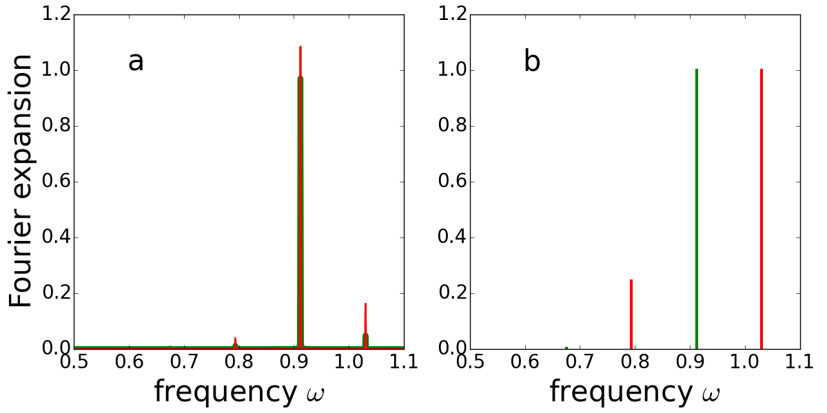
Figure 1: Fourier expansion vs. frequency for $x_{0},y_{0},p_{y0}=0,0,0.18$, power order $n_{s}=5$, a:$w_{x0}$ (green) $w_{y0}$ (red) b:$v_{1}$ (green),$v_{2}$ (red). $w_{x0},w_{y0}$ are normalized so their initial values are 1. $w_{x0}$ (green) and $w_{y0}$ (red) are nearly parallel except $w_{y0}$ has a second lower peak at $\omega_{2}=1.03$ with $|\widetilde{w}_{y001}|=0.164$, higher than the second peak for $w_{x0}$, $|\widetilde{w}_{x001}|=0.049$. Hence the two vectors are independent, so it is possible to choose a set of vector basis ($v_{1}$, $v_{2}$) that they are nearly orthogonal in the frequency space. This is carried out as shown in Section 3 to calculate $\{a_{11},a_{12}\}$,$\{a_{21},a_{22}\}$ in Eq.(3.5), with the sum over $n$, $m$ in Eq.(3.1) limited to only over the 6 lines in Table I. The result is shown in b, with $|\widetilde{v}_{1nm}|$ (green) and $|\widetilde{v}_{2nm}|$ (red).

n	m	$\omega=n\omega_{1}+m\omega_{2}$	$|\widetilde{w}_{x0nm}|$	$|\widetilde{w}_{y0nm}|$
1	0	0.9120	0.972	1.089
0	1	1.0303	0.049	0.164
2	-1	0.7937	0.013	0.043
0	0	0.0000	0.012	0.014
2	0	1.8240	0.006	0.006
3	-1	1.7057	0.000	0.005

Table 1: Absolute value of Fourier expansion coefficients

6.2 Numerical Examples

Since our goal is to find the solution without using the numerical forward integration, we shall illustrate the iteration procedure to find the action-angle variables using an example Eq.(1.1) with initial condition $E=H=1/12\approx.083$3, $x_{0},y_{0},p_{y0}=$ $0,0,0.18$ ($p_{x0}$ is determined from $H$ in Eq.(1.1)). However, in order to check the result, we need to compare the iteration progress and the result with the forward integration. Hence we first present the result obtained by forward integration, represented by a trajectory $x^{(e)},p_{x}^{(e)},y^{(e)},p_{y}^{(e)}$.

Following Section 3, we search for two linear combinations for which $v_{1}$, $v_{2}$ nearly represent two independent rigid rotations, i.e., with two different frequencies and with minimized fluctuation. We take $n_{s}=5,n_{v}=2$. The Fourier transform of $w_{x0},w_{y0}$, with the trajectory $x^{(e)},p_{x}^{(e)},y^{(e)},p_{y}^{(e)}$ is shown in Fig.1a. In Table 1 we list the top 6 peaks with their frequencies, indices ${n,m}$, and peak heights. The spectrum of $v_{1}$, $v_{2}$ with fluctuation minimized is shown in Fig.1b. The fluctuation of $|v_{2}|$ mainly due to the line at $\omega=0.7937$ is to be further reduced by the procedure prescribed in Section 6.1.

But our goal is to find the solution without the forward integration, so we shall not use the linear combination obtained this way. Instead, in the following example, we start the iteration procedure from the initial trial linear combinations $\{a_{11},a_{12}\}$,$\{a_{21},a_{22}\}$ given by Eq.(2.6) derived from the differential equations at the initial position. And, we introduce normalized action-angle variables $\bar{v}_{1}\equiv v_{1}/r_{1},\bar{v}_{2}\equiv v_{2}/r_{2}$, so in many of the following plots of spectrum the fluctuation is relative to $|\bar{v}_{1}|\approx 1,|\bar{v}_{2}|\approx 1$ (see Eq.(5.6)).

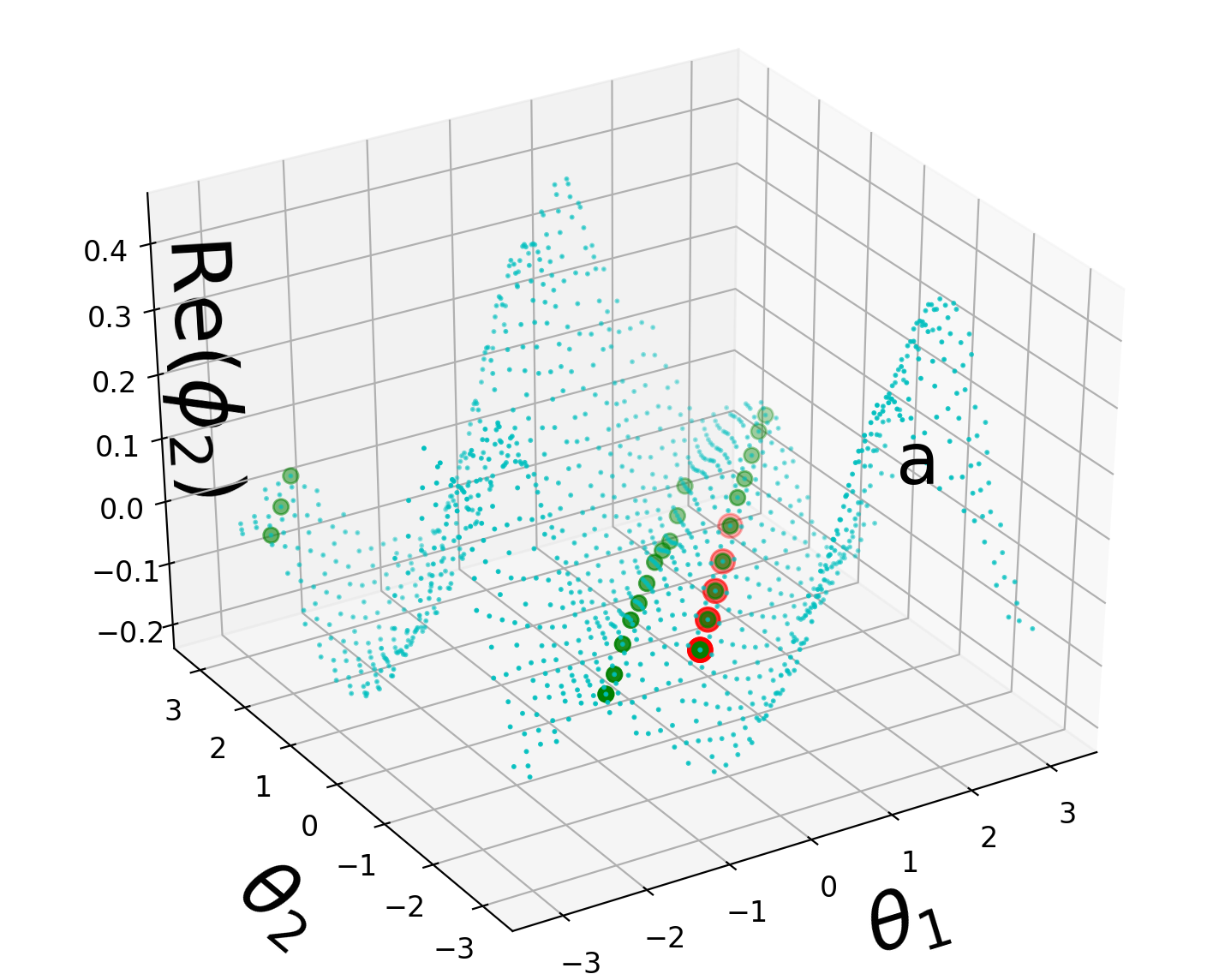
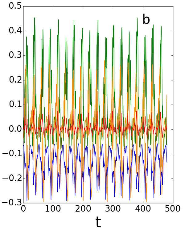
Figure 2: For $x_{0},y_{0},p_{y0}=0,0,0.18$, linear combinations based on differential equations at the initial position, a: $\text{Re(}\phi_{2})$ calculated from Eq.(4.3) as the rigid rotations $v_{1}^{(0)}$, $v_{2}^{(0)}$ in Eq.(4.4) pass through the $\theta_{1}^{(0)}$, $\theta_{2}^{(0)}$ plane. The first 5 points (red), and first 24 points (green) show how the trajectory scans through the plane. b: $\text{{Re}}\phi_{1}$ (blue), $\text{{Im}}\phi_{1}$(red), $\text{{Re}}\phi_{2}$(green), $\text{{Im}}\phi_{2}$ (orange) as function of $t$.

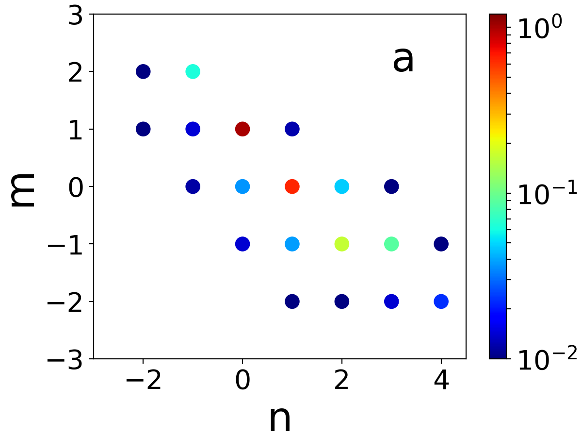
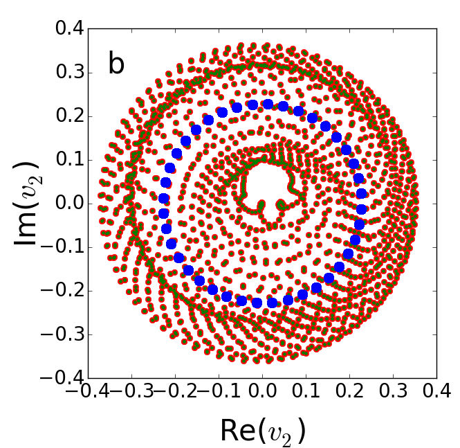
Figure 3: a. Fourier expansion vs. indices of $\bar{v}_{2}^{(1)}$ in iteration 1, calculated by Eq.(5.5). The red dot at $n,m=1,0$ in Fig.3a corresponds to $\widetilde{\theta}_{21,-1}$ in Eq.(5.6). Notice the top 3 peaks $n,m=${0,1},{1,0}{2,-1} in Fig.3a correspond to the top 3 peaks with intensity of 1,0.64, 0.17 in Fig.4b at $\omega_{2}=1.0984$, $\omega_{1}=0.8600,$ $2\omega_{1}-\omega_{2}=0.6215$ respectively. b: phase space $v_{2}^{(0)}$(blue), $v_{2}^{(1)}$ (red, calculated from Eq.(5.6) ), $v_{2}^{(1)}$(green): from $v_{1}^{(1)}$, $v_{2}^{(1)}$, the inverse function of Eq.(4.1) are used to find the trajectory $x^{(1)},p_{x}^{(1)},y^{(1)},p_{y}^{(1)}$, which in turn are used to calculate $w_{x0},w_{y0}$ and their Fourier transform $\widetilde{w}_{jnm}$, and $\widetilde{v}_{lnm}$ in Eq.(3.2) of Section 3, using the initial trial linear combinations $\{a_{11},a_{12}\}$,$\{a_{21},a_{22}\}$ of iteration 1. The results are used to calculate $v_{1}^{(1)}$, $v_{2}^{(1)}$ again and plotted in b as green dots for a double check because they should coincide with the red dots.

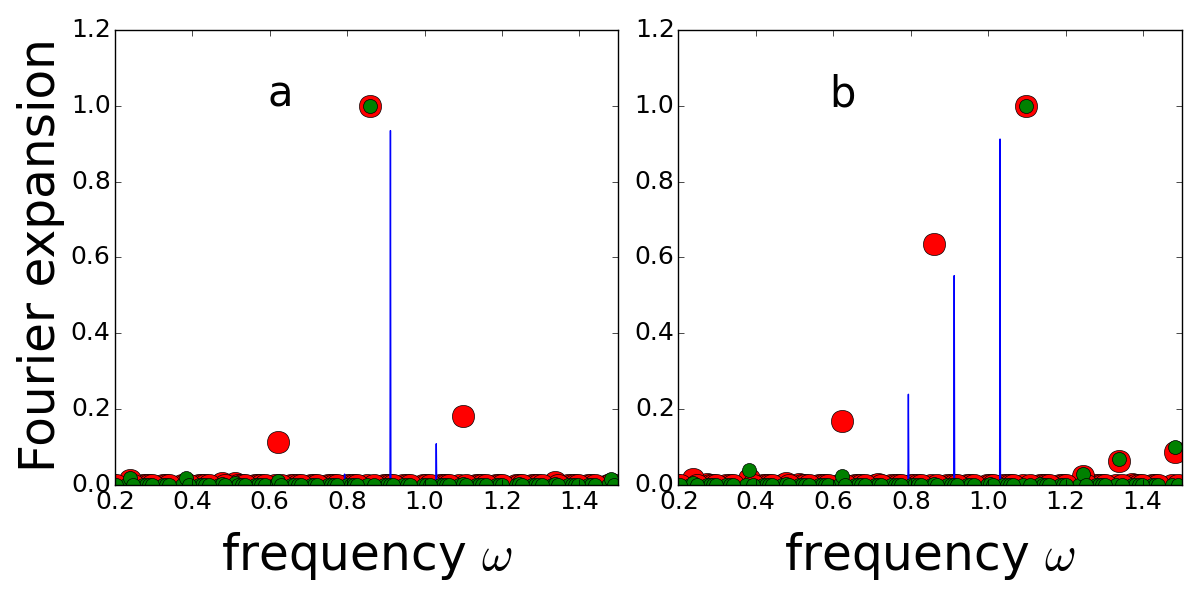
Figure 4: Fourier expansion vs. frequency, iteration 1, a:$\bar{v}_{1}$ b: $\bar{v}_{2}$. Red dots are $\widetilde{\theta}_{1nm}$ $\widetilde{\theta}_{2nm}$ of Eq.(5.4), Eq.(5.5), green dots are $\widetilde{v}_{lnm}$ in Eq.(3.2) using linear combinations Eq.(3.5) for minimized fluctuation in iteration 1, i.e., the initial linear combination of iteration 2; blue lines are $\bar{v}_{2}^{(e)}$ in iteration 1. For the red dots, the intensity 1 at $\omega_{2}=1.098$ , the dominating line of $\bar{v}_{2}^{(1)}$, is not much more than the intensity 0.64 at $\omega_{1}=0.8600$ while our goal is to find $\bar{v}_{2}^{(1)}$ dominated by the line at $\omega_{2}$. So $\bar{v}_{2}^{(1)}$ can hardly represent a perturbation to the rigid rotation. The fact $\omega_{1},\omega_{2}=0.860,1.098$ is different from $\omega_{1},\omega_{2}=0.912,1.030$ obtained from the forward integration as given in Table I is because the errors in the initial trial linear combination, and the perturbation calculation. As the iteration progresses, $\omega_{1},\omega_{2}$ approaches $0.912,1.030$. The frequencies of the red dots $\bar{v}_{2}^{(1)}$ have large errors relative to the blue lines $\bar{v}_{2}^{(e)}$ showing $\bar{v}_{2}^{(1)}$ is a poor approximation. The green dots are dominated by $\omega_{1}$ and $\omega_{2}$ in Fig.4a and Fig.4b respectively. The rigid rotations determined by the new linear combinations should be single lines at $\omega_{1}$ and $\omega_{2}$ in Fig.4a and 4b, hence the rigid rotation is a good approximation of green dots $\bar{v}_{2}^{(1)}$, expressed in terms of the new linear combination derived in iteration 1.

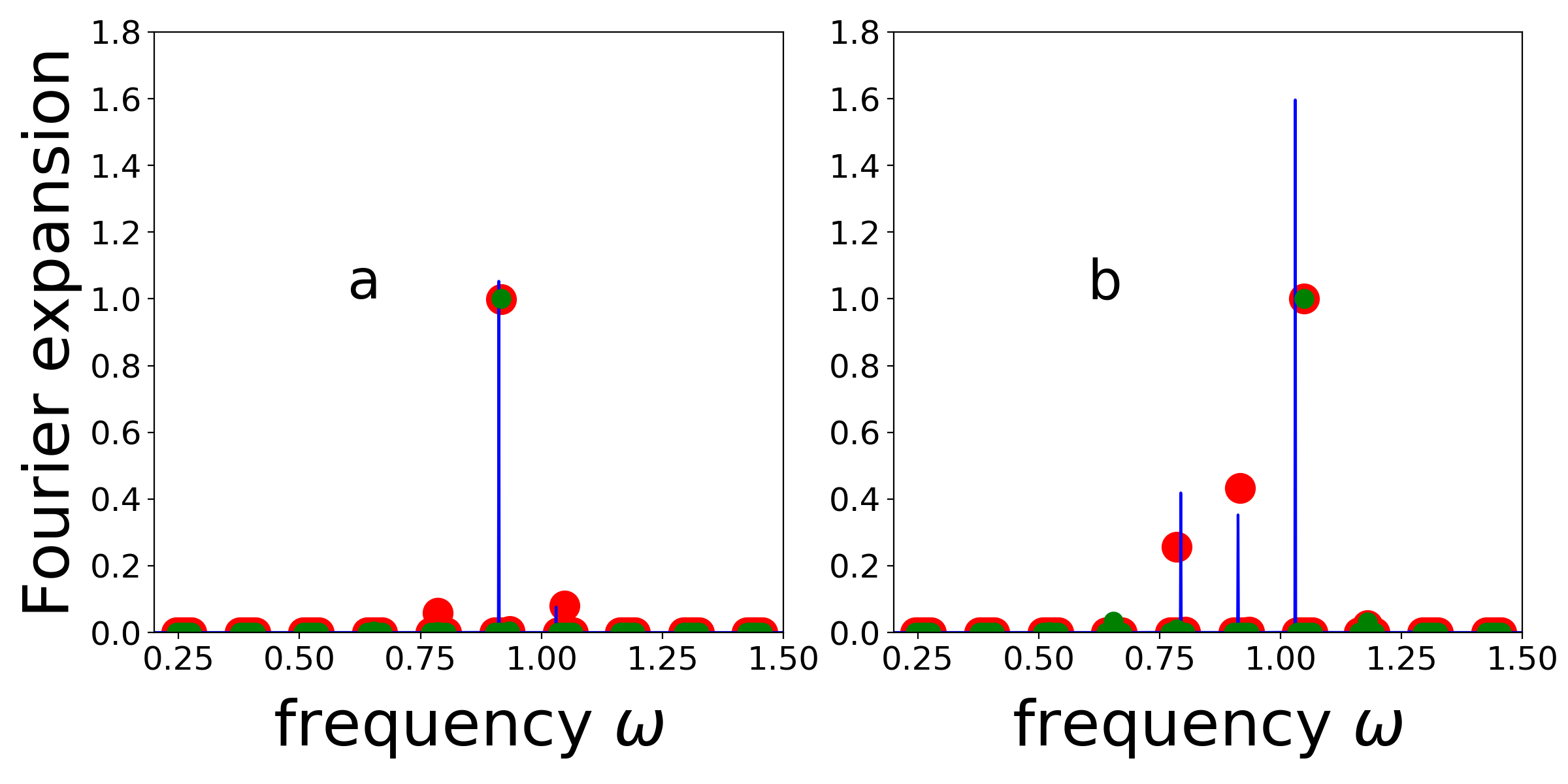
Figure 5: Fourier expansion vs. frequency, iteration 2, a:$\bar{v}_{1}$ b:$\bar{v}_{2}$. $v_{1}^{(1)}$, $v_{2}^{(1)}$ (red) are calculated from $v_{1}^{(0)}$, $v_{2}^{(0)}$ by steps prescribed in Section 4 and 5 based on the linear combinations $\{a_{11},a_{12}\}$,$\{a_{21},a_{22}\}$ derived in iteration 1. Again the blue lines are $\bar{v}_{1}^{(e)}$ , $\bar{v}_{2}^{(e)}$. Now the blue line at $\omega_{2}=1.03$ is much higher than $\omega_{1}=0.912$ in Fig.5b showing that in iteration 2, the rigid rotation $v_{2}^{(0)}$ (a single line at $\omega_{2}$) is a better approximation than in iteration 1 when compared with Fig.4b, even though it is still a poor approximation because the line at $\omega_{1}$ is still more than 25% of the line at $\omega_{2}$. The red dot at $\omega_{1}=0.917$ in Fig.5b is still 40% of $\omega_{2}=1.048$, showing $\bar{v}_{2}^{(1)}$ is still a poor approximation of the accurate solution $\bar{v}_{2}^{(e)}$ (the blue lines). Clearly this is due to the fact $v_{2}^{(0)}$ in iteration 2 is still a poor approximation. But the frequencies of the red dots are much more closer to the blue lines than Fig.4. Again the green dots show a new set of linear combinations with minimized fluctuation for $\bar{v}_{1}^{(1)}$, $\bar{v}_{2}^{(1)}$ in iteration 2 , which now is the zeroth order approximation $\bar{v}_{1}^{(0)}$, $\bar{v}_{2}^{(0)}$ in iteration 3.

Then we apply the perturbation theory of Section 4 to calculate the zeroth order $v_{1}^{(0)}$, $v_{2}^{(0)}$, and $\phi_{1}$, $\phi_{2}$ in Eq.(4.3). A comparison of Fig.2a with Fig.2b helps to understand how the trajectory passes the $\theta_{1}^{(0)}$, $\theta_{2}^{(0)}$ plane.

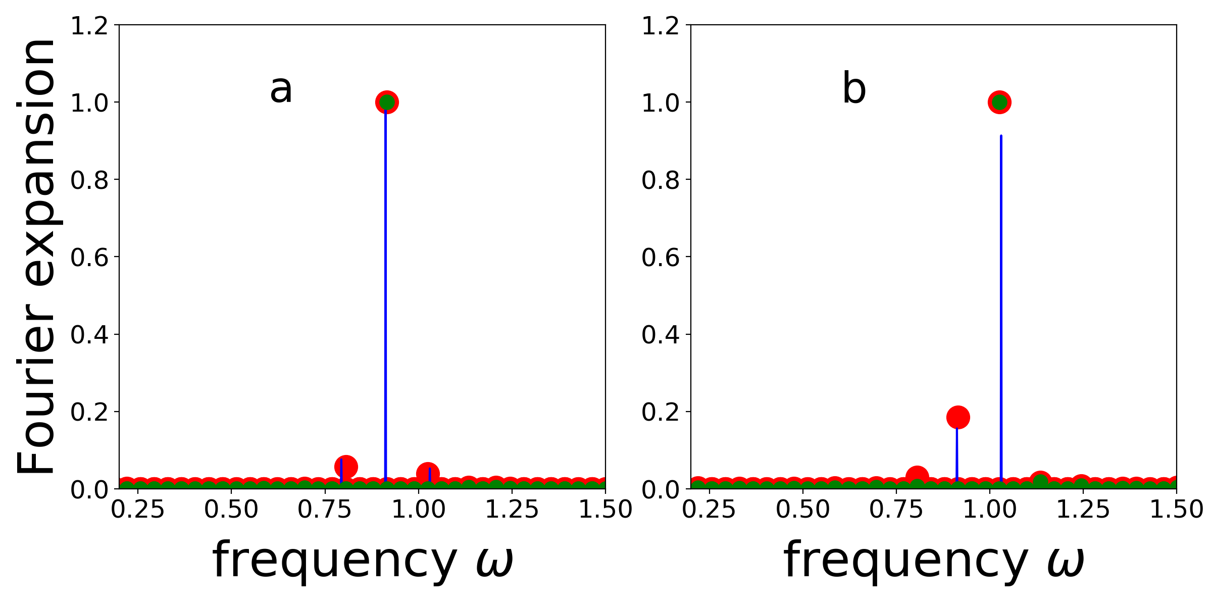
Figure 6: Fourier expansion vs. frequency, iteration 3, a:$\bar{v}_{1}$ b:$\bar{v}_{2}$. The Fourier expansion of $\bar{v}_{1}^{(1)}$, $\bar{v}_{2}^{(1)}$ (red dots) of iteration 3 show they are dominated by red dots $\omega_{1}$ and $\omega_{2}$ respectively. The fluctuation in $|\bar{v}_{2}^{(1)}|$ is the line at $\omega_{1}=0.915$ with height 0.19, much smaller the main line at $\omega_{2}=1.025$ with height 1. All the red, green dots and blue lines are dominated by $\omega_{1}$ and $\omega_{2}$ respectively in Fig.6a,b, showing the iteration is converging.

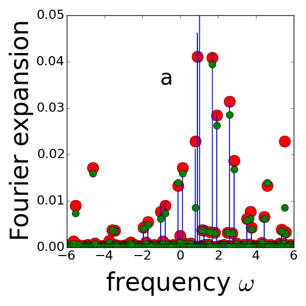
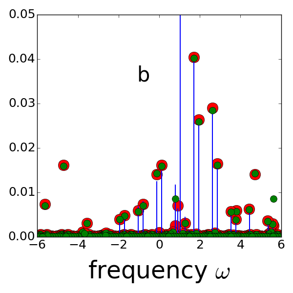
Figure 7: Fourier expansion vs. frequency. a:$\bar{v}_{2}$ iteration 4, b: $\bar{v}_{2}$ iteration 5

Figure 8: Fourier expansion vs. frequency. a :$\bar{v}_{2}$ iteration 6, b: $\bar{v}_{2}$ iteration 7. The fluctuation (about 4%) is calculated to be in agreement with the forward integration, i.e.,$\bar{v}_{1}^{(1)}\approx\bar{v}_{1}^{(e)},\bar{v}_{2}^{(1)}\approx\bar{v}_{2}^{(e)}$, accurate to about 0.6%. This is visible when compare the red dots (the first order approximation based on the rigid rotations) with the blue lines (the forward integration). The red dots almost coincide with the green dots (the new linear combinations for $v_{2}^{(1)}$at the end of iteration 7) indicates convergence of the iteration.

If we increase the left eigenvectors to $w_{x0},w_{y0},w_{x1},w_{y1}$ $(n_{v}=4)$, we can obtained $|v_{2}|$ with less fluctuation. However, because the vectors $w_{x1},w_{y1}$ are also dominated by $\omega_{1}$, $\omega_{2}$, components of frequency other than $\omega_{1}$, $\omega_{2}$ are small. The inclusion of $w_{x1},w_{y1}$ in the minimization process often results in large contribution from $w_{x1},w_{y1}$ to suppress other components, even if the fluctuation is small, thus makes the iteration convergence slow or even stopped before the dominance of the main frequency components $\omega_{1}$, $\omega_{2}$ in $v_{1},v_{2}$ is established respectively. Hence we take $n_{v}=2$ at first so the iteration converges quickly.

The 2-D Fourier transform of $\bar{v}_{2}^{(1)}$ vs. indices based on the steps in Section 5 in iteration 1 is shown in Fig.3a, and, as function of frequency, is shown in Fig.4b as the red dots. In Fig.3b we show $v_{2}^{(1)}$ in the phase space of $\text{Re}(v_{2})$, $\text{{Im}}(v_{2})$ (red dots). The blue dots are $v_{2}^{(0)}$. Fig.3b shows the deviation of $v_{2}^{(1)}$ from $v_{2}^{(0)}$ is so large that it is hardly a perturbation to the rigid rotation. This is observed in Fig.4b too. In Fig.4b, the frequencies of the red dots $\bar{v}_{2}^{(1)}$ have large errors relative to the blue lines $\bar{v}_{2}^{(e)}$also showing it is a very poor approximation.

With this provision, the next step is to find the new linear combinations $\{a_{11},a_{12}\}$,$\{a_{21},a_{22}\}$ by the minimization procedure from Eq.(3.3) to Eq.(3.5). The spectrum of $\bar{v}_{1}^{(1)}$, $\bar{v}_{2}^{(1)}$ obtained by the new linear combination of iteration 1 is shown as green dots in Fig.4a and Fig.4b, they are close to rigid rotations. Therefore the rigid rotations represented by the new linear combinations serves as the zeroth order approximation in iteration 2. This completes the iteration 1.

The iteration 2 follows the same steps. Now the zeroth order approximation $v_{1}^{(0)}$, $v_{2}^{(0)}$, calculated from the linear combinations derived in iteration 1, and represent single lines at $\omega_{1}$ and $\omega_{2}$ respectively in Fig.5a, 5b, are close to the first order approximation in iteration 1. Fig.5b shows that in iteration 2, the rigid rotation $v_{2}^{(0)}$ is a better approximation than in iteration 1 even though it is still a poor approximation. Clearly because of this, Fig.5b also shows $\bar{v}_{2}^{(1)}$(red) is still a poor approximation of the accurate solution (blue).

The spectrum in Fig.6a,b shows $v_{1}^{(1)}$, $v_{2}^{(1)}$ in iteration 3 are well represented by rigid rotations. To reduce the fluctuation due to other harmonics such as $2\omega_{1}-\omega_{2}=0.805$ in iteration 3, we repeat the minimization procedure of Section 3 in iteration 2 with increased number of left eigenvectors $n_{v}=4$ in Eq.(3.2). The green dots in Fig.5a,b and the plots of iteration 3 in Fig.6a,b are all based on linear combinations calculated with $n_{v}=4$. Fig.6a,b shows the iteration is converging.

Since the $v_{1}^{(1)}$ always has much smaller fluctuation than $v_{2}^{(1)}$, in the following iterations we only show the spectrum of $v_{2}^{(1)}$. Because the fluctuation decreases rapidly to lower than a few percent of the main peaks of height 1, we change the axis scale to 5% maximum, and increased the frequency range to show wider noise spectral range. These plots in iteration 4-7 are shown in Fig.7-8, showing the fluctuation spectrum pattern converges. Consider the very complicated noise spectrum in Fig.8b, the extremely detailed agreement between the red dots (square matrix solution) and the blue lines (the forward integration) is very pronounced.

In Fig.8b the final convergent result $v_{1}^{(e)}$, $v_{2}^{(e)}$ have fluctuation over the rigid rotations of about 4%. We see $v_{1}^{(1)}\approx v_{1}^{(e)}$, $v_{2}^{(1)}\approx$ $v_{2}^{(e)}$,

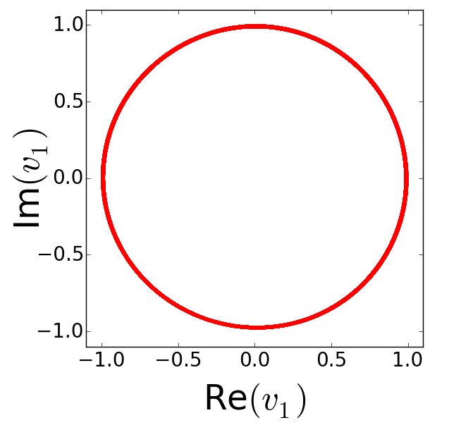
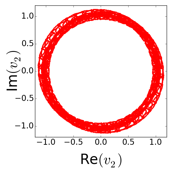
Figure 9: left:$v_{1}^{(e)}$ , right:$v_{2}^{(e)}$ iteration 7. $v_{1}^{(e)}$ is nearly a perfect circle, $v_{2}^{(e)}$ has a fluctuation of the radius about 4%, as expected from the spectrum in Fig.8b.

accurate to about 0.6%, much less than 4%. This observation allows us to derive a set of much more accurate KAM invariants $\bar{v}_{01}$,$\bar{v}_{02}$, as will be explained in the Section 7.

Result of iteration: Fig.9 show $v_{1}^{(e)}$, $v_{2}^{(e)}$ of the last linear combination. Fig.10 shows $v_{2}^{(1)}$, in agreement with $v_{2}^{(e)}$ in Fig.9. Fig.11 shows the upper half $y,p_{y}$ plane of the Poincare surface section with x crosses zero, showing the result from square matrix gives much better agreement with forward integration.

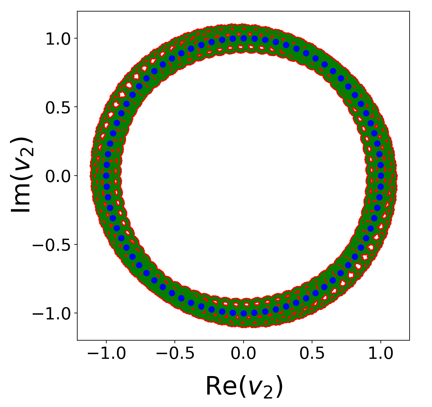
Figure 10: phase space trajectories of $v_{2}^{(1)}$ calculated by Eq.(5.6) in iteration 7 with maximum $n$ and $m$ between {${-40,40}$}, in clear agreement with Fig.9b. A comparison with Fig.3b shows how the iteration reduces the fluctuation.

6.3 Results of solution for other initial conditions

When the iteration procedure is applied to initial coordinates for $x_{0}=0$, and various {$y_{0},p_{y0}$}, the results from power order $n_{s}=5$ (green) similar to Fig.11 are shown in Fig.12, showing much better agreement with forward integration (red) than the contours (magenta) from canonical perturbation theory Gustavson (6) calculated at power order 8, even near $y_{0},p_{y0}=\{0,0.14\}$.

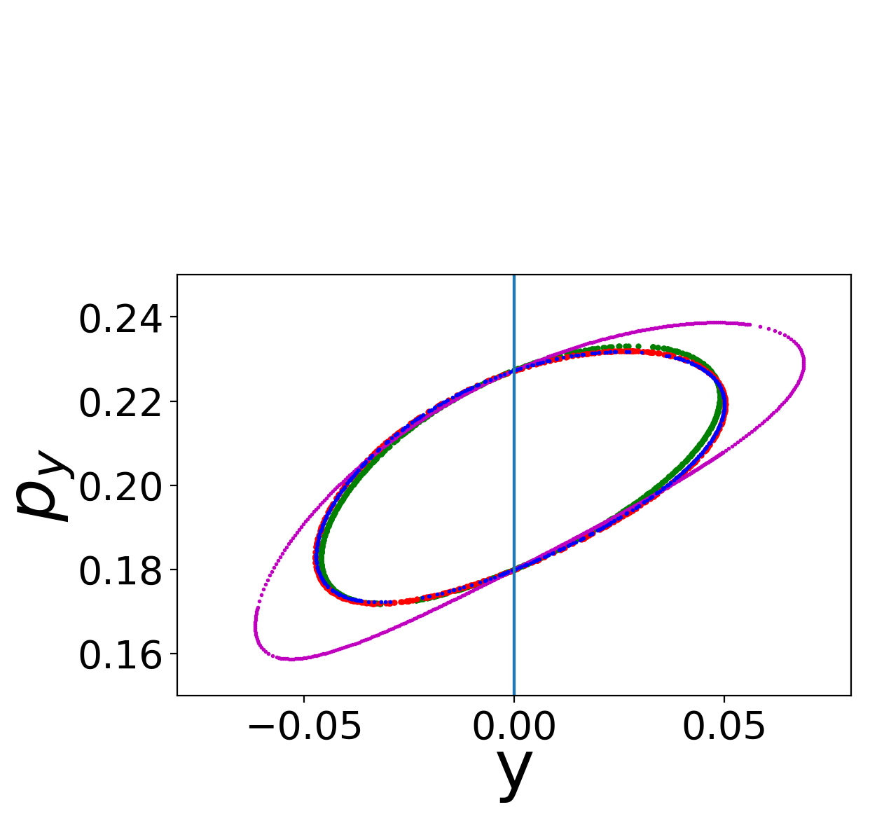
Figure 11: Poincare surface section $y,p_{y}$with $x=0$. Because energy conservation, for energy E=0.0833, $p_{x}$ is determined from $x,y,p_{y}$, so when the KAM invariant survives the trajectory passes through a surface in the 3 dimension space of $x,y,p_{y}$. The trajectory crosses the x=0 plane in one direction in the top half plane into the region $x>0$, and later crosses the x=0 and comes back into the $x<0$ region. Thus the trajectory crosses the plane by a curve shown as red points (the forward integration $v_{1}^{(e)}$, $v_{2}^{(e)}$). The green dots are the coordinates calculated from the inverse function of Eq.(4.1) with $v_{1}^{(1)}$, $v_{2}^{(1)}$ obtained in the last iteration with power order $n_{s}=5$, corresponding to the red dots in Fig.8b, in good agreement with the forward integration $v_{1}^{(e)}$, $v_{2}^{(e)}$. The magenta dots are obtained from the well known canonical perturbation theory based on Table IV in Gustavson (6), calculated to 8th power order. The result from square matrix clearly gives much better agreement with forward integration. The blue dots are $\bar{v}_{01}$,$\bar{v}_{02}$, to be introduced in Section 7, in nearly perfect agreement with forward integration (red).

Notice that at {0,0.14} the contour calculated from the canonical perturbation theory at 8th power order jumps across the separatrix and is marked as black contour circling around the fixed points near {0.25,0} and(-0.3,0), while the numerical solution (red), the square matrix solution (green) and the more accurate solution $\bar{v}_{02}$ (blue, to be introduced later in Section 7) remain at the same side, around the fixed points near {0,0.2} and {0,-0.2}.

In Fig.12, the square matrix calculation uses power order $n_{s}=5$ for all the initial positions. Except at $y_{0},p_{y0}=\{0,0.14\}$, the error bar of $\bar{v}_{02}$ increases to 2.5%, so we increases power order to $n_{s}=7$ to reduce the error bar to about 1%. When we continue from {0,0.14} to {0,0.135} the iteration procedure is no longe convergent for $n_{s}=7$ and $n_{v}=4$.

When we keep $n_{s}=5$, we can continue from {0,0.14} down to as low as {0, 0.127} but the error bar of $\bar{v}_{02}$ has increased to 10%. Numerical forward integration starts to show irregular behavior at {0, 0.123745}, so the curve on the x=0 Poincare surface section jumps back and forth between the two sides of the seperatrix. But this value is sensitive to numerical integrator setup.

7 Transform Rotation with Fluctuation into KAM invariant

The procedure in Section 6 results in the action-angle variables $v_{1}^{(1)}$,$v_{2}^{(1)}$, which represent rigid rotations with 4% fluctuation. This fluctuation is related to the power order of the square matrix $n_{s}=5$ and the number of left eigenvectors used in the linear combination $n_{v}=4$, and the initial $y_{0},p_{y0}=0,0.18$. However, the comparison with forward integration shows only 0.6% error. After the last iteration, $v_{1}^{(0)}$,$v_{2}^{(0)}$ represents rigid rotations without fluctuation but it is not accurate solution. $v_{1}^{(1)}$, $v_{2}^{(1)}$ represents more accurate solution but with larger fluctuation. This allows us to derive a much more accurate KAM invariant than $v_{1}^{(1)}$,$v_{2}^{(1)}$ using the relation between $v_{1}^{(1)}$,$v_{2}^{(1)}$ and $v_{1}^{(0)}$,$v_{2}^{(0)}$.

The relation is derived as follows. Substitute the expression of zeroth order action Eq.(4.4) into the first order action Eq.(5.6), use the normalized actio-angle variables $\bar{v}_{1},\bar{v}_{2}$, substitute $e^{i\theta_{1}^{(0)}(t)},e^{i\theta_{2}^{(0)}(t)}$ by $\bar{v}_{1}^{(0)},\bar{v}_{2}^{(0)}$ , and use the iteration result of $v_{1}^{(1)}\approx v_{1}^{(e)}$, $v_{2}^{(1)}\approx v_{2}^{(e)}$ as shown at the end of Section 6.2 about Fig.8, we get

$$\begin{split}&\bar{v}_{1}^{(e)}\approx\bar{v}_{1}^{(1)}=\bar{v}_{1}^{(0)}e^{i\thinspace\sum_{n,m}\widetilde{\theta}_{1nm}(\bar{v}_{1}^{(0)})^{n}(\bar{v}_{2}^{(0)})^{m}}\\ &\bar{v}_{2}^{(e)}\approx\bar{v}_{2}^{(1)}=\bar{v}_{2}^{(0)}e^{i\thinspace\sum_{n,m}\widetilde{\theta}_{2nm}(\bar{v}_{1}^{(0)})^{n}(\bar{v}_{2}^{(0)})^{m}}\end{split}$$ (7.1)

Eq.(7.1) expresses the exact action in terms of the zeroth order action. Given the zeroth order function $\bar{v}_{1}^{(0)},\bar{v}_{2}^{(0)}$ as rigid rotations, Eq.(7.1) gives $\bar{v}_{1}^{(1)},\bar{v}_{2}^{(1)}$ as perturbed rigid rotations with fluctuation, which more closely represents the motion $\bar{v}_{1}^{(e)},\bar{v}_{2}^{(e)}$ .

Notice the first approximate equal signs in the left hand side of Eq.(7.1) are valid only if $\bar{v}_{1}^{(0)},\bar{v}_{2}^{(0)}$ are on unit circle, we can use the inverse function of Eq.(7.1) to test if $\bar{v}_{1}^{(0)}(t),\bar{v}_{2}^{(0)}(t)$ do represent rigid rotations. In other words, the inverse function $\bar{v}_{1}^{(0)},\bar{v}_{2}^{(0)}$ of Eq.(7.1), expressed as a function of $\bar{v}_{1}^{(e)},\bar{v}_{2}^{(e)}$, as polynomials of $x,p_{x},y,p_{y}$, should be a much more accurate action approximation than $\bar{v}_{1}^{(1)},\bar{v}_{2}^{(1)}$. In addition, when we are searching for KAM invariants we always assume $x,p_{x},y,p_{y}$ are on the exact trajectory, so in the following we replace the notation $\bar{v}_{1}^{(e)},\bar{v}_{2}^{(e)}$ by $\bar{v}_{1},\bar{v}_{2}$.

To calculate this inverse function, we first neglect the small terms in the right hand side of Eq.(7.1) so we have $\bar{v}_{1}^{(0)}\approx\bar{v}_{1}^{(1)}\approx\bar{v}_{1}^{(e)}=\bar{v}_{1}$, $\bar{v}_{2}^{(0)}\approx\bar{v}_{2}^{(1)}\approx\bar{v}_{2}^{(e)}=\bar{v}_{2}$. Replace $\bar{v}_{1}^{(0)},\bar{v}_{2}^{(0)}$ by $\bar{v}_{1},\bar{v}_{2}$ in the exponents in Eq.(7.1), we found

$$\begin{split}&\bar{v}_{01}=\bar{v}_{1}^{(0)}=\bar{v}_{1}^{(e)}e^{-i\thinspace\sum_{n,m}\widetilde{\theta}_{1nm}(\bar{v}_{1}^{(0)})^{n}(\bar{v}_{2}^{(0)})^{m}}\approx\\ &\bar{v}_{1}e^{-i\thinspace\sum_{n,m}\widetilde{\theta}_{1nm}(\bar{v}_{1})^{n}(\bar{v}_{2})^{m}}\approx\bar{v}_{1}\thinspace(1-i\thinspace\sum_{n,m}\widetilde{\theta}_{1nm}(\bar{v}_{1})^{n}(\bar{v}_{2})^{m})\\ &\bar{v}_{02}=\bar{v}_{2}^{(0)}=\bar{v}_{2}^{(e)}e^{-i\thinspace\sum_{n,m}\widetilde{\theta}_{2nm}(\bar{v}_{1}^{(0)})^{n}(\bar{v}_{2}^{(0)})^{m}}\approx\\ &\bar{v}_{2}e^{-i\thinspace\sum_{n,m}\widetilde{\theta}_{2nm}(\bar{v}_{1})^{n}(\bar{v}_{2})^{m}}\approx\bar{v}_{2}\thinspace(1-i\thinspace\sum_{n,m}\widetilde{\theta}_{2nm}(\bar{v}_{1})^{n}(\bar{v}_{2})^{m})\end{split}$$ (7.2)

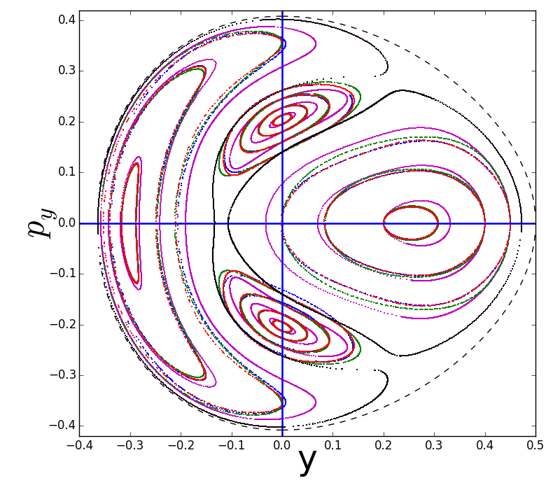
Figure 12: Poincare surface section $x=0$ for trajectory with initial condition $x_{0}=0$, and $y_{0},p_{y0}=$ {0, 0.195}, {0,0.18}, {0,0.16}, {0,0.14}, {0.2,0}, {0.4,0}, {0.45,0}. Red: forward numerical integration. Green: constant contours of $v_{1},v_{2}$ given by Eq.(4.1). Blue: constant contours of $\bar{v}_{01},\bar{v}_{02}$ given by Eq.(7.2) (see Section 7). Magenta: contours from Table IV of Gustavson (6). Notice at {0,0.14} the contour calculated from the canonical perturbation theory at 8th power order jumps across the separatrix and is marked as black contour. The dashed black line is the energy limit $\frac{1}{2}p_{x}^{2}+\frac{1}{2}y^{2}-\frac{1}{3}y^{3}=E$ for $E=0.0833$. The solution for $y_{0},p_{y0}=$ {0.2,0}, {0.4,0} and {0,0.195} are found in the same way as {0,0.18}. The solutions for {0,0.16} can also be found the sam way, but here it is found by starting the iteration with the linear combinations obtained from {0,0.18} case. The dominance of the $\omega_{2}$ line in $v_{2}^{(1)}$ is established from the start so the convergence process starts immediately. The 0.14 case follows the solution for 0.16 by first going to 0.145, then 0.143. The solution for {0.45,0} is found by starting iteration from the solution for {0.4,0}. We see that the blue curve (see Section 7) starts to show a small deviation from the numerical integration near $y_{0},p_{y0}=$ {0,-0.14} but not at {0,0.14}. This asymmetry is due to the fact the solution process is not symmetric for upper and lower half plane: we start the initial point at {0, 0.14}, not {0,-0.14} so the errors are different between upper and lower half plane.

Here we denote the $\bar{v}_{1}^{(0)},\bar{v}_{2}^{(0)}$ using a different notation $\bar{v}_{01},\bar{v}_{02}$ to indicate the distinction between the variable $\bar{v}_{1}^{(0)},\bar{v}_{2}^{(0)}$ in Eq.(7.1) and $\bar{v}_{01},\bar{v}_{02}$ in Eq.(7.2). In Eq.(7.1) we consider them as a simple expression as in Eq.(4.4) representing rigid rotations in the phase space of $\theta_{1}^{(0)},\theta_{2}^{(0)}$. Then Eq.(7.1) gives a more accurate representation of the motion, as two independent perturbed rigid rotations. In Eq.(7.1) $\bar{v}_{1}^{(0)},\bar{v}_{2}^{(0)}$ are calculated from Eq.(4.4) as function of $\theta_{1}^{(0)},\theta_{2}^{(0)}$, or $x^{(0)},p_{x}^{(0)},y^{(0)},p_{y}^{(0)}$ , while $\bar{v}_{1}^{(1)},\bar{v}_{2}^{(1)}$ are function of $x^{(1)},p_{x}^{(1)},y^{(1)},p_{y}^{(1)}$. Eq.(7.1) is used to find solution without forward integration.

As a comparison, in Eq.(7.2), $\bar{v}_{01},\bar{v}_{02}$ are more complicated function of $x,p_{x},y,p_{y}$ than $\bar{v}_{1},\bar{v}_{2}$ , they represent the much more accurate approximation to rigid rotations. In Eq.(7.2) $\bar{v}_{1},\bar{v}_{2}$ are calculated from Eq.(4.1) as function of $x^{(e)},p_{x}^{(e)},y^{(e)},p_{y}^{(e)}=x,p_{x},y,p_{y}$. Eq.(7.2) gives a KAM invariant for a known solution.

In Fig.13a we show the phase space of $\bar{v}_{02}$ as given by Eq.(7.2). Clearly this represents a rigid rotation with much less fluctuation than $\bar{v}_{2}^{(1)}$ as shown in Fig.9b. We remark here that clearly the solution $\bar{v}_{01},\bar{v}_{02}$ in Eq.(7.2) is not a Taylor expansion, its exponent is a function with both positive and negative powers of the polynomials $\bar{v}_{1},\bar{v}_{2}$, i.e., a Laurent series of $\bar{v}_{1},\bar{v}_{2}$. When we carry out Taylor expansion of $\bar{v}_{02}$ to $n_{s}=5$ order, the result has a huge fluctuation. Our numerical test shows only if we expand up to power order of 17 we are able to keep the fluctuation to 0.6% as shown in Fig.13a. From this, we expect the solution should be in the general form Eq.(7.2), where the power order $n_{s}=5$ of $\bar{v}_{1},\bar{v}_{2}$ is not required to be very high to reach high precision. It is not appropriate to use power expansion for the KAM invariant $\bar{v}_{01},\bar{v}_{02}$ to achieve high precision.

To compare the errors of several action-angle variables we derived, in Fig.13b we plot the details of the contours of the x=0 Poincare surface section for initial $y_{0},p_{y0}=0,0.18$ in Fig.12. It is very clear from this plot, $\bar{v}_{2}^{(1)}$ (green) the first order approximation is much more close to the forward integration (red) than the magenta curve derived from the canonical perturbation theory. The more accurate $\bar{v}_{02}$ (blue) given by Eq.(7.2) is even much more close to the red than the green. This demonstrates the high precision of KAM invariant Eq.(7.2).

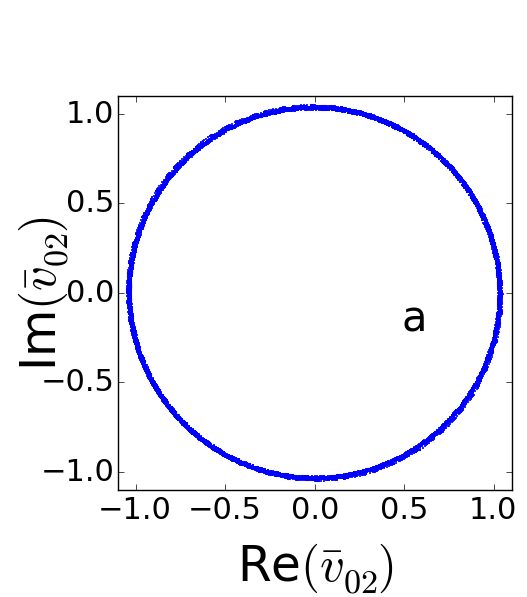
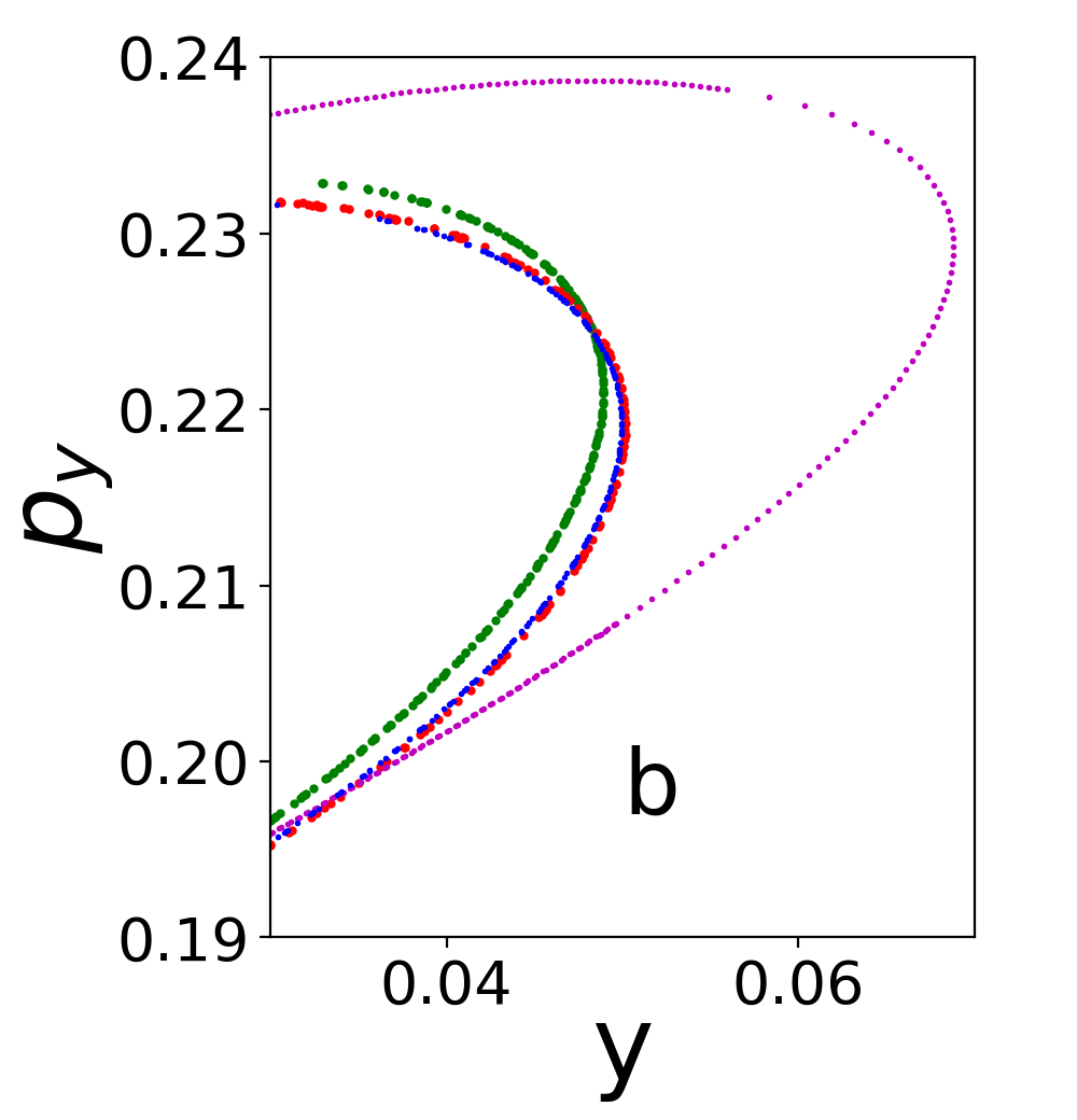
Figure 13: For the trajectory with initial condition $x_{0}=0$, and $y_{0},p_{y0}=$ {0,0.18}, power order $n_{s}=5$. a. phase space of $\bar{v}_{02}$ given by Eq.(7.2) with $x,p_{x},y,p_{y}$ in $\bar{v}_{1},\bar{v}_{2}$ calculated from forward integration, nearly a perfect circle.  b. A detailed magnified part in Fig.12 for error comparison of different KAM invariant approximations on Poincare surface section $x=0$. Red: forward numerical integration. Green: constant contours of $v_{1},v_{2}$ given by Eq.(4.1). Blue: constant contours of $\bar{v}_{02}$ given by Eq.(7.2). Magenta: contours from Table IV of Gustavson (6) based on canonical perturbation theory. Clearly $\bar{v}_{02}$ is much more precise than previous theory.

8 Conclusion

We developed a perturbation theory for nonlinear dynamics on resonances based on using the liner combinations of left eigenvectors in the degenerate Jordan chains of a square matrix as the zeroth order approximate action-angle variables to find highly accurate approximation of the KAM invariants. The solution is not in the form of a power series, but in the form of an exponential function with rational function as its exponent, more like a Laurent series rather than a Taylor series. To achieve high precision, the required power order for the action-angle variables in the exponent is much less stringent than the required power order for the power series expansion to achieve the same precision.

The solution is found by an iteration procedure. In each iteration step, we need to solve a set of linear equations to improve the accuracy. Numerical study shows, for the example of Henon-Heiles problem, the iteration converges in much of the region where the KAM invariants persist. While the result of the canonical perturbation theory in the example still gives contours in the region where the orbits fall into chaotic behavior (see Fig.10 of Gustavson (6) and the black curve in Fig.12 of Section 6.3), the iteration based on the square matrix method is no longer convergent when approaching the stability boundary. This gives a way to get information about the stability boundary, and also raised the question about the relation of the convergence region and the stability boundary. Whether there is an analytical answer on this question remains to be a very interesting and important issue.

While for the canonical perturbation theory the measure of the perturbation is given by the amplitude of the nonlinear terms, for the perturbation theory developed for square matrix the measure of the perturbation is given by the fluctuation relative to the amplitude of the action-angle variables in the initial trial iteration. Hence when approaching the stability boundary the reduction of the step size can reduce the fluctuation and may lead to convergence and improve the precision with increased power order of $n_{s}$, or increased number of left eigenvectors $n_{v}$. Hence the convergence and precision seem to be determined by the ratio of the increase of the fluctuation over the step size, instead of being determined by the amplitude of the perturbation only. In this sense the meaning of perturbation here is different from the conventional meaning, or may be even beyond perturbation, hence may have the potential to explore the area with increased amplitude or perturbation.

References

• (1) A. J. Lichtenberg and M. A. Lieberman, Regular and Chaotic Dynamics (Springer, New York, 1992).
• (2) Henk W. Broer, Bulletin (New Series) of The American Mathematical Society, Volume 41, Number 4, Pages 507-521, 2004
• (3) Jürgen Pöschel, ”A Lecture on the Classical KAM Theorem”, Proc. Symp. Pure Math. 69 (2001) 707–732
• (4) V. Arnold. “Small denominators, 1: Mappings of the circumference onto itself.” AMS Translations, 46:213–288, 1965 (Russian original published in 1961).
• (5) C. Eugene Wayne, “An Introduction to KAM Theory”, http://math. bu. edu/people/cew/preprints/introkam. pdf
• (6) F. G. Gustavson, The Astronomical Journal Volume 71, Number 8 October 1966
• (7) B. Chirikov, Physics Reports (Review Section of Physics Letters) 52, No. 5(1979)263-379. North-Holland Publishing Company
• (8) A. J. Dragt, “Lie Algebraic Methods For Charged Particle Optics”, AIP Conf. Proc. 177, 261 (1988).
• (9) M. Berz, Proceedings of the 1989 Particle Accelerator Conference, Chicago, Illinois (IEEE, New York, 1989), p. 1419.
• (10) A. Chao, “Lie Algebra Techniques for Nonlinear Dynamics”, Report No. SLAC-PUB-9574, 2002, Chap. 9.
• (11) E. Forest, M. Berz, and J. Irwin, Normal form methods for complicated periodic systems: A complete solution using differential algebra and lie operators, Part. Accel. 24, 91 (1989).
• (12) M. Brown, W. D. Neumann, “Proof of the Poincare-Birkhoff fixed-point theorem”. Michigan Math. J. Vol. 24, 1977, p. 21–31.
• (13) L. H. Yu and B. Nash, Linear Algebraic Method For Nonlinear Map Analysis, In Proceedings Of PAC09, Vancouver, BC, Canada, 2009, 3862.
• (14) L. H. Yu, Phys. Rev. Accel. Beams Volume 20, Pages 034001 (Year 2017).
• (15) Michel Henon, Carl Heiles, The Astronomical Journal Volume 69, Number 1 February 1964
• (16) R. J. Glauber, “Coherent And Incoherent States Of Radiation Field”, Phys. Rev. 131, 2766 (1963)
• (17) E. C. G. Sudarshan, “Equivalence of Semiclassical and Quantum Mechanical Descriptions of Statistical Light Beams”, Phys. Rev. Lett. 10, 277 (1963).