Fractional diffusion equation description of an open anomalous heat conduction set-up

Aritra Kundu1, Cédric Bernardin2, Keji Saito3, Anupam Kundu4, Abhishek Dhar5 1,4,5International Centre for Theoretical Sciences, Bengaluru, India
2Université Côte d’Azur, CNRS, LJADNice Cedex 02, France
3Department of Physics, Keio University, Yokohama 223-8522, Japan
$^1$aritrak@icts.res.in,$^2$Cedric.BERNARDIN@unice.fr,$^3$saitoh@rk.phys.keio.ac.jp,
$^4$anupam.kundu@icts.res.in,$^5$abhishek.dhar@icts.res.in,
Abstract

We provide a stochastic fractional diffusion equation description of energy transport through a finite one-dimensional chain of harmonic oscillators with stochastic momentum exchange and connected to Langevian type heat baths at the boundaries. By establishing an unambiguous finite domain representation of the associated fractional operator, we show that this equation can correctly reproduce equilibrium properties like Green-Kubo formula as well as non-equilibrium properties like the steady state temperature and current. In addition, this equation provides the exact time evolution of the temperature profile. Taking insights from the diffusive system and from numerical simulations, we pose a conjecture that these long-range correlations in the steady state are given by the inverse of the fractional operator. We also point out some interesting properties of the spectrum of the fractional operator. All our analytical results are supplemented with extensive numerical simulations of the microscopic system.

1 Introduction

Energy transport across an extended system is a fundamental non-equilibrium phenomena which is often described by the phenomenological Fourier law. This law leads to the heat equation for the evolution of the temperature field T(y,t)𝑇𝑦𝑡T(y,t), which in one dimension is given by

tT(y,t)=(κ/c)y2T(y,t),subscript𝑡𝑇𝑦𝑡𝜅𝑐superscriptsubscript𝑦2𝑇𝑦𝑡\partial_{t}T(y,t)=({\kappa}/c)\partial_{y}^{2}T(y,t), (1)

where c𝑐c is the specific heat capacity and κ𝜅{\kappa} the heat conductivity (assumed, for simplicity to be temperature independent). This equation plays a central role in understanding heat transport through macroscopic materials in several contexts. However, various studies have established that for a large class of one and two dimensional systems with momentum conservation, energy transport is not diffusive but super-diffusive — this is referred to as anomalous transport [1, 2, 3]. There are several signatures of anomalous transport which include the super-diffusive spreading of localized heat pulses and the form of spatio-temporal correlations in equilibrium set-up as well as diverging thermal conductivity in non-equilibrium (boundary driven) set-up . Unlike diffusive transport, currently there are no general framework to understand these features of anomalous transport completely except for a recent development based on non-linear fluctuating hydrodynamics theory [4, 5, 6, 7]. This theory, based on some phenomenological assumptions, provides a framework to understand the super-diffusive energy transport in a wide class of one-dimensional anharmonic classical Hamiltonian systems such as the Fermi-Pasta-Ulam-Tsingou (FPUT) system and hard-particle gases [4, 5, 7, 6, 8, 9].

One picture that has emerged from many studies is that, for systems with anomalous transport, the standard heat diffusion equation has to be replaced by some fractional diffusion equation [1, 10, 11, 12, 13, 14, 15]. A particular model of anomalous transport where some rigorous results have been obtained is that of the harmonic chain whose Hamiltonian dynamics is supplemented by a stochastic part that keeps the conservation laws (volume, energy, momentum) intact — we will refer this model as the harmonic chain momentum exchange (HCME) model. For the infinite HCME system, it was shown exactly that at equilibrium the energy current autocorrelation has a t1/2similar-toabsentsuperscript𝑡12\sim t^{-1/2} decay [16]. It was also shown that, in contrast to Eq. (1), in infinite volume, the evolution of a localized energy perturbation e(y,t)𝑒𝑦𝑡e(y,t), is described by a non-local fractional diffusion equation te(y,t)=κ¯(Δ)3/4e(y,t)subscript𝑡𝑒𝑦𝑡¯𝜅superscriptΔ34𝑒𝑦𝑡\partial_{t}e(y,t)=-\bar{\kappa}(-\Delta)^{3/4}e(y,t), where κ¯¯𝜅\bar{\kappa} is some constant which depends on microscopic parameters [14]. The fractional Laplacian operator (Δ)3/4superscriptΔ34(-\Delta)^{3/4} in the infinite space is defined by its Fourier spectrum: |q|3/2superscript𝑞32|q|^{3/2} which for the normal Laplacian operator Δy2Δsubscriptsuperscript2𝑦-\Delta\equiv-\partial^{2}_{y} is q2superscript𝑞2q^{2}.

While most of the studies in HCME model consider evolution in infinite systems, it is also of interest to study transport across a finite system connected to two reservoirs of different temperatures at its two ends. For diffusive systems in this set-up, the heat equation continues to describe both non-equilibrium steady state (NESS) and time-dependent properties. However, for anomalous transport, it is a priori not clear how to write a corresponding evolution equation in a finite domain. Since we expect this evolution to be governed by a fractional Laplacian which is a non-local operator, it is difficult to guess its representation in a finite system from its representation in the infinite system. Note that in the finite system one has to include the effects of the boundary conditions which are important as the operator itself is non-local. Hence, extending its definition to a finite domain is a non-trivial problem. Several studies have addressed this problem of obtaining and studying fractional diffusion description in finite domain [17, 18, 19].

In this paper we study heat transfer across the HCME model connected to two reservoirs at its two ends. It has been observed and proved that in this model, heat current scaling with system size is anomalous and the steady state temperature profile is inherently non-linear [1, 11, 20]. In the present work we provide a fractional equation description of the anomalous heat transfer both in the stationary as well as in the non-stationary state. Using this fractional description we derive new results related to evolution of temperature profile, equilibrium current fluctuations and to two point correlations in NESS. Below we summarise the main results of our work along with the plan of the paper:

  • In Sec. (2) we first review previous studies on the HCME model. These studies show that the macroscopic time evolution of two-point correlations is described by a set of coupled local linear PDEs [11, 12]. Starting from these PDEs, it can be shown that they naturally give rise to an evolution equation for the temperature profile T(y,τ)𝑇𝑦𝜏T(y,\tau)

    τT(y,τ)=κ¯𝕃T(y,τ),subscript𝜏𝑇𝑦𝜏¯𝜅𝕃𝑇𝑦𝜏\partial_{\tau}T(y,\tau)=-\bar{\kappa}~{}\mathbb{L}T(y,\tau),

    governed by a fractional Laplacian 𝕃𝕃\mathbb{L} defined in a finite domain, where τ𝜏\tau is a scaled time (see later). The operator 𝕃𝕃\mathbb{L} is defined in the domain 0y10𝑦10\leq y\leq 1 through it’s action

    𝕃ϕn(y)=λn3/4ϕn(y)𝕃subscriptitalic-ϕ𝑛𝑦superscriptsubscript𝜆𝑛34subscriptitalic-ϕ𝑛𝑦\mathbb{L}\phi_{n}(y)=\lambda_{n}^{3/4}\phi_{n}(y)

    on the complete Neumann basis y|ϕn=ϕn(y)=2cos(nπy)inner-product𝑦subscriptitalic-ϕ𝑛subscriptitalic-ϕ𝑛𝑦2𝑛𝜋𝑦\langle y|\phi_{n}\rangle=\phi_{n}(y)=\sqrt{2}\cos(n\pi y) for n1𝑛1n\geq 1 and y|ϕ0=ϕ0(y)=1inner-product𝑦subscriptitalic-ϕ0subscriptitalic-ϕ0𝑦1\langle y|\phi_{0}\rangle=\phi_{0}(y)=1 with λn=(nπ)2subscript𝜆𝑛superscript𝑛𝜋2\lambda_{n}=(n\pi)^{2}. Using this representation, we show that one can recover the exact results [11] for the steady state temperature and current profiles in the HCME.

  • Next in Sec. (3) we discuss the time evolution of the temperature profile, starting from an arbitrary initial profile, to the long-time NESS profile. In order to solve the fractional diffusion equation with Dirichlet boundary conditions for arbitrary time we are required to find the eigenvalues and eigenvectors of the fractional operator 𝕃𝕃\mathbb{L} with Dirichlet boundary conditions. We describe an efficient procedure to compute this eigensystem. We also provide a detailed discussion of some properties of the eigensystem that distinguish them from the eigensystem of the normal Laplacian operator with the same boundary conditions.

  • Inspired by the fluctuating equations for energy evolution in diffusive systems[21, 22], in Sec. (4) we extend the definition of the fractional equation to include fluctuations and noise in equilibrium such that fluctuation-dissipation relation holds locally.

  • Using the fluctuating fractional equation description, in Sec. (4.2), we first verify the validity of the equilibrium Green-Kubo relation in finite systems where we encounter some interesting mathematical identities that we establish numerically. This motivates and enables us to study the long-range correlations in NESS in Sec. (4.4), where we propose a conjecture on the relation between these correlations and the Green’s function of the operator 𝕃𝕃\mathbb{L}.

  • Finally, in Sec. (5) we conclude our paper.

2 Definition of Model and survey of earlier results

We consider the so-called harmonic chain momentum exchange model (HCME), which considers an added stochastic component in the usual Hamiltonian dynamics of a harmonic chain. The stochastic part is such that it preserves volume, momentum and energy conservation but the other conserved variables of the harmonic chain are no longer conserved. Thus the stochastic model restores ergodicity while preserving the important conservation laws. Here we are interested in the open system where the system is driven by two Langevin-type heat baths. Specifically we consider a system consisting of N𝑁N particles and attached to two heat baths. The Hamiltonian plus heat bath part of the dynamics is described by the following equations

q˙i=subscript˙𝑞𝑖absent\displaystyle\dot{q}_{i}= pi,p˙i=ω2(qi+12qi+qi1),1<i<N,formulae-sequencesubscript𝑝𝑖subscript˙𝑝𝑖superscript𝜔2subscript𝑞𝑖12subscript𝑞𝑖subscript𝑞𝑖11𝑖𝑁\displaystyle~{}p_{i}~{},~{}~{}\dot{p}_{i}=\omega^{2}(q_{i+1}-2q_{i}+q_{i-1}),~{}~{}1<i<N,
p˙1=subscript˙𝑝1absent\displaystyle\dot{p}_{1}= ω2(q22q1)λp1+2λTLηL,superscript𝜔2subscript𝑞22subscript𝑞1𝜆subscript𝑝12𝜆subscript𝑇𝐿subscript𝜂𝐿\displaystyle~{}\omega^{2}(q_{2}-2q_{1})-\lambda p_{1}+\sqrt{2\lambda T_{L}}\eta_{L}, (2)
p˙N=subscript˙𝑝𝑁absent\displaystyle\dot{p}_{N}= ω2(qN12qN)λpN+2λTRηR,superscript𝜔2subscript𝑞𝑁12subscript𝑞𝑁𝜆subscript𝑝𝑁2𝜆subscript𝑇𝑅subscript𝜂𝑅\displaystyle~{}\omega^{2}(q_{N-1}-2q_{N})-\lambda p_{N}+\sqrt{2\lambda T_{R}}\eta_{R}~{},

where {qi,pi}subscript𝑞𝑖subscript𝑝𝑖\{q_{i},p_{i}\}, i=1,2,N𝑖12𝑁i=1,2\ldots,N, are the positions and momenta of the particles, TL,TRsubscript𝑇𝐿subscript𝑇𝑅T_{L},T_{R} are the temperatures of the left and the right Langevin baths and ηL,ηRsubscript𝜂𝐿subscript𝜂𝑅\eta_{L},\eta_{R} are Gaussian white noise terms. Additionally there is a stochastic noise, such that the momenta of nearest neighbour particles are exchanged (i.e pi+1pisubscript𝑝𝑖1subscript𝑝𝑖p_{i+1}\leftrightarrow p_{i}) at a rate γ𝛾\gamma. For this model the two point correlation functions satisfy a closed set of equations.

Following [12] let us denote the possible correlation matrices by 𝐔i,j=qiqjsubscript𝐔𝑖𝑗delimited-⟨⟩subscript𝑞𝑖subscript𝑞𝑗{\bf U}_{i,j}=\langle q_{i}q_{j}\rangle,𝐕i,j=pipjsubscript𝐕𝑖𝑗delimited-⟨⟩subscript𝑝𝑖subscript𝑝𝑗{\bf V}_{i,j}=\langle p_{i}p_{j}\rangle, and 𝐙i,j=qipjsubscript𝐙𝑖𝑗delimited-⟨⟩subscript𝑞𝑖subscript𝑝𝑗{\bf Z}_{i,j}=\langle q_{i}p_{j}\rangle. One can show that the time evolution of these correlation functions is given by linear equations involving only these set of correlations and source terms arising from the boundary driving [12]. Let us also define the correlation 𝐳i,j+=(𝐙i,j𝐙i1,j+𝐙j,i𝐙j1,i)/2subscriptsuperscript𝐳𝑖𝑗subscript𝐙𝑖𝑗subscript𝐙𝑖1𝑗subscript𝐙𝑗𝑖subscript𝐙𝑗1𝑖2{\bf z}^{+}_{i,j}=\left({\bf Z}_{i,j}-{\bf Z}_{i-1,j}+{\bf Z}_{j,i}-{\bf Z}_{j-1,i}\right)/2. The most interesting physical observables involve the correlations Ti=𝐕iisubscript𝑇𝑖subscript𝐕𝑖𝑖T_{i}={\bf V}_{ii}, which can be taken as the definition of local temperature and the energy current J=ω2𝐳i,i+1++(γ/2)(𝐕i+1,i+1𝐕i,i)𝐽superscript𝜔2subscriptsuperscript𝐳𝑖𝑖1𝛾2subscript𝐕𝑖1𝑖1subscript𝐕𝑖𝑖J=\omega^{2}{\bf z}^{+}_{i,i+1}+(\gamma/2)~{}({\bf V}_{i+1,i+1}-{\bf V}_{i,i}). In the N𝑁N\to\infty limit, one observes that the fields Tisubscript𝑇𝑖T_{i} and 𝐳i,j+subscriptsuperscript𝐳𝑖𝑗{\bf z}^{+}_{i,j} have the scaling forms Ti(t)=T(i/N,t/N3/2)subscript𝑇𝑖𝑡𝑇𝑖𝑁𝑡superscript𝑁32T_{i}(t)=T(i/N,t/N^{3/2}) and 𝐳i,j+=1NC(|ij|)/N1/2,(i+j)/(2N),t/N3/2){\bf z}^{+}_{i,j}=\frac{1}{\sqrt{N}}C(|i-j|)/{N}^{1/2},(i+j)/(2N),t/N^{3/2}). In terms of the following scaling variables x=|ij|/N1/2,y=(i+j)/(2N),τ=t/N3/2formulae-sequence𝑥𝑖𝑗superscript𝑁12formulae-sequence𝑦𝑖𝑗2𝑁𝜏𝑡superscript𝑁32x=|i-j|/{N}^{1/2},y=(i+j)/(2N),\tau=t/N^{3/2}, it has been shown in [12] that the fields T(y,τ)𝑇𝑦𝜏T(y,\tau) and C(x,y,τ)𝐶𝑥𝑦𝜏C(x,y,\tau) satisfy the following coupled set of PDEs:

γ2x4C(x,y,τ)superscript𝛾2superscriptsubscript𝑥4𝐶𝑥𝑦𝜏\displaystyle\gamma^{2}\partial_{x}^{4}C(x,y,\tau) =ω2y2C(x,y,τ),absentsuperscript𝜔2superscriptsubscript𝑦2𝐶𝑥𝑦𝜏\displaystyle=\omega^{2}\partial_{y}^{2}C(x,y,\tau),
yT(y,τ)subscript𝑦𝑇𝑦𝜏\displaystyle\partial_{y}T(y,\tau) =2γxC(x,y,τ)|x0,absentevaluated-at2𝛾subscript𝑥𝐶𝑥𝑦𝜏𝑥0\displaystyle=-2\gamma\partial_{x}C(x,y,\tau)|_{x\to 0}, (3)
τT(y,τ)subscript𝜏𝑇𝑦𝜏\displaystyle\partial_{\tau}T(y,\tau) =ω2yC(x,y,τ)|x0,absentevaluated-atsuperscript𝜔2subscript𝑦𝐶𝑥𝑦𝜏𝑥0\displaystyle=\omega^{2}\partial_{y}C(x,y,\tau)|_{x\to 0},

with boundary conditions C(x,0,τ)=C(x,1,τ)=0,C(,y,τ)=0,x3C(0,y,τ)=0formulae-sequence𝐶𝑥0𝜏𝐶𝑥1𝜏0formulae-sequence𝐶𝑦𝜏0superscriptsubscript𝑥3𝐶0𝑦𝜏0C(x,0,\tau)=C(x,1,\tau)=0,C(\infty,y,\tau)=0,\partial_{x}^{3}C(0,y,\tau)=0 and T(0,τ)=TL𝑇0𝜏subscript𝑇𝐿T(0,\tau)=T_{L} and T(1,τ)=TR𝑇1𝜏subscript𝑇𝑅T(1,\tau)=T_{R} where, the domain of variables are x[0,)𝑥0x\in[0,\infty) and y[0,1]𝑦01y\in[0,1] [note that in [12] y(1,1)𝑦11y\in(-1,1)]. To study the time-evolution of the fields C(x,y,τ)𝐶𝑥𝑦𝜏C(x,y,\tau) and T(y,τ)𝑇𝑦𝜏T(y,\tau), one has to subtract the steady state solutions Css(x,y)subscript𝐶𝑠𝑠𝑥𝑦C_{ss}(x,y) and Tss(y)subscript𝑇𝑠𝑠𝑦T_{ss}(y) of the above equations (whose explicit forms are given in [11]). The boundary conditions suggest that one expand the difference fields using the complete Dirichlet basis y|αn=αn(y)=2sin(nπy)inner-product𝑦subscript𝛼𝑛subscript𝛼𝑛𝑦2𝑛𝜋𝑦\langle y|\alpha_{n}\rangle=\alpha_{n}(y)=\sqrt{2}\sin(n\pi y) for n1𝑛1n\geq 1

C(x,y,τ)Css(x,y)=n=1C^n(x,τ)αn(y),𝐶𝑥𝑦𝜏subscript𝐶𝑠𝑠𝑥𝑦superscriptsubscript𝑛1subscript^𝐶𝑛𝑥𝜏subscript𝛼𝑛𝑦\displaystyle C(x,y,\tau)-C_{ss}(x,y)=\sum_{n=1}^{\infty}\hat{C}_{n}(x,\tau)\alpha_{n}(y), (4)
T(y,τ)Tss(y)=f(y,τ)=n=1f^n(τ)αn(y).𝑇𝑦𝜏subscript𝑇𝑠𝑠𝑦𝑓𝑦𝜏superscriptsubscript𝑛1subscript^𝑓𝑛𝜏subscript𝛼𝑛𝑦\displaystyle T(y,\tau)-T_{ss}(y)=f(y,\tau)=\sum_{n=1}^{\infty}\hat{f}_{n}(\tau)\alpha_{n}(y)~{}. (5)

Following [12] one then gets (see B) the following matrix equation for the evolution of the components fnsubscript𝑓𝑛f_{n}:

f^˙n=subscript˙^𝑓𝑛absent\displaystyle\dot{\hat{f}}_{n}= κ¯k=1𝕃nkf^k,n=1,2,,,formulae-sequence¯𝜅superscriptsubscript𝑘1subscript𝕃𝑛𝑘subscript^𝑓𝑘𝑛12\displaystyle-\bar{\kappa}\sum_{k=1}^{\infty}\mathbb{L}_{nk}\hat{f}_{k},~{}~{}~{}~{}n=1,2,\ldots,\infty,~{} (6)
where,where\displaystyle~{}\text{where},~{} 𝕃nk=[𝒯Λ3/4𝒯]nk,subscript𝕃𝑛𝑘subscriptdelimited-[]𝒯superscriptΛ34superscript𝒯𝑛𝑘\displaystyle\mathbb{L}_{nk}=\left[\mathcal{T}\Lambda^{3/4}\mathcal{T^{\dagger}}\right]_{nk}, (7)

with 𝒯nl=αn|ϕl=01𝑑yαn(y)ϕl(y)subscript𝒯𝑛𝑙inner-productsubscript𝛼𝑛subscriptitalic-ϕ𝑙superscriptsubscript01differential-d𝑦subscript𝛼𝑛𝑦subscriptitalic-ϕ𝑙𝑦\mathcal{T}_{nl}=\langle\alpha_{n}|\phi_{l}\rangle=\int_{0}^{1}dy\alpha_{n}(y)\phi_{l}(y), where ϕm(y)=2cos(mπy)subscriptitalic-ϕ𝑚𝑦2𝑚𝜋𝑦\phi_{m}(y)=\sqrt{2}\cos(m\pi y) for m>0𝑚0m>0, ϕ0(y)=1subscriptitalic-ϕ0𝑦1\phi_{0}(y)=1 and Λml=λmδmlsubscriptΛ𝑚𝑙subscript𝜆𝑚subscript𝛿𝑚𝑙\Lambda_{ml}=\lambda_{m}\delta_{ml} is a diagonal matrix with λn=(nπ)2subscript𝜆𝑛superscript𝑛𝜋2\lambda_{n}=(n\pi)^{2}. The constant κ¯=ω3/2/(22γ)¯𝜅superscript𝜔3222𝛾\bar{\kappa}={\omega^{3/2}}/{(2\sqrt{2\gamma})}. Therefore, the function f(x,τ)𝑓𝑥𝜏f(x,\tau) with homogeneous boundaries f(0,τ)=f(1,τ)=0𝑓0𝜏𝑓1𝜏0f(0,\tau)=f(1,\tau)=0 satisfies,

τf(y,τ)=κ¯𝕃f(y,τ).subscript𝜏𝑓𝑦𝜏¯𝜅𝕃𝑓𝑦𝜏\displaystyle\partial_{\tau}f(y,\tau)=-\bar{\kappa}\mathbb{L}f(y,\tau). (8)

From Eq. (7), one notices that 𝕃nksubscript𝕃𝑛𝑘\mathbb{L}_{nk} can be written as

𝕃nk=αn|𝕃|αk=αn|[m=0λm3/4|ϕmϕm|]|αk,n,k=1,2,,formulae-sequencesubscript𝕃𝑛𝑘quantum-operator-productsubscript𝛼𝑛𝕃subscript𝛼𝑘brasubscript𝛼𝑛delimited-[]superscriptsubscript𝑚0superscriptsubscript𝜆𝑚34ketsubscriptitalic-ϕ𝑚brasubscriptitalic-ϕ𝑚ketsubscript𝛼𝑘for-all𝑛𝑘12\mathbb{L}_{nk}=\langle\;\alpha_{n}\;|\mathbb{L}|\;\alpha_{k}\;\rangle=\langle\;\alpha_{n}\;|\left[\sum_{m=0}^{\infty}\lambda_{m}^{3/4}|\;\phi_{m}\;\rangle\langle\;\phi_{m}\;|\right]|\;\alpha_{k}\;\rangle,~{}~{}\forall~{}~{}n,k=1,2,\ldots,\infty

which allows us to identify the action of the operator 𝕃𝕃\mathbb{L} acting on the set of basis functions ϕmsubscriptitalic-ϕ𝑚\phi_{m} (which satisfy Neumann boundary conditions):

𝕃|ϕm=λm3/4|ϕm.𝕃ketsubscriptitalic-ϕ𝑚superscriptsubscript𝜆𝑚34ketsubscriptitalic-ϕ𝑚\displaystyle\mathbb{L}|\;\phi_{m}\;\rangle=\lambda_{m}^{3/4}|\;\phi_{m}\;\rangle~{}. (9)

It is important to notice that the above representation of the operator 𝕃𝕃\mathbb{L} is not the “spectral fractional Laplacian with Dirichlet boundary conditions” which would consist to replace ϕnsubscriptitalic-ϕ𝑛\phi_{n} by αnsubscript𝛼𝑛\alpha_{n} in (9). This definition has been mentioned in [1] and a more mathematically rigorous derivation has been obtained [19]. The above results imply that the temperature field T(y,τ)𝑇𝑦𝜏T(y,\tau) evolves according to the fractional equation

τT(y,τ)=κ¯𝕃T(y,τ)=𝕃κ¯T(y,τ),subscript𝜏𝑇𝑦𝜏¯𝜅𝕃𝑇𝑦𝜏subscript𝕃¯𝜅𝑇𝑦𝜏\displaystyle\partial_{\tau}T(y,\tau)=-\bar{\kappa}\mathbb{L}T(y,\tau)=-\mathbb{L}_{\bar{\kappa}}T(y,\tau)~{}, (10)

where we have defined 𝕃κ¯=κ¯𝕃subscript𝕃¯𝜅¯𝜅𝕃\mathbb{L}_{\bar{\kappa}}=\bar{\kappa}\mathbb{L} and the steady state is required to satisfy the condition 𝕃κ¯Tss(y)=0subscript𝕃¯𝜅subscript𝑇𝑠𝑠𝑦0\mathbb{L}_{\bar{\kappa}}T_{ss}(y)=0. To describe the evolution of the temperature profile, one is specifically interested in finding the eigenvectors of the operator 𝕃𝕃\mathbb{L} which satisfy Dirichlet boundary conditions. This can be obtained by diagonalizing the infinite-dimensional matrix in Eq. (7). Let the eigenvector components of this matrix be denoted by ψn(m)subscriptsuperscript𝜓𝑚𝑛\psi^{(m)}_{n}, corresponding to eigenvalue μnsubscript𝜇𝑛\mu_{n}, so that k𝕃mkψn(k)=μnψn(m)subscript𝑘subscript𝕃𝑚𝑘subscriptsuperscript𝜓𝑘𝑛subscript𝜇𝑛subscriptsuperscript𝜓𝑚𝑛\sum_{k}\mathbb{L}_{mk}\psi^{(k)}_{n}=\mu_{n}\psi^{(m)}_{n}. Then the eigenvector in the position basis is given by ψn(y)=mψn(m)αm(y)subscript𝜓𝑛𝑦subscript𝑚superscriptsubscript𝜓𝑛𝑚subscript𝛼𝑚𝑦\psi_{n}(y)=\sum_{m}\psi_{n}^{(m)}\alpha_{m}(y). In Sec. 3 we provide an alternate and more efficient method of computing eigenvalues and eigenvectors. This method involves finding roots of a transcendental equation and avoids diagonalization of infinite dimensional matrices. We also discuss various properties of the spectrum there. We now describe several results that follow for the steady state and the time evolution towards it.

2.1 Steady state results

Let us write the steady state temperature in the form

Tss(y)=T¯+δTΘ(y),subscript𝑇𝑠𝑠𝑦¯𝑇𝛿𝑇Θ𝑦T_{ss}(y)=\overline{T}+\delta T~{}\Theta(y), (11)

where T¯=(TL+TR)/2¯𝑇subscript𝑇𝐿subscript𝑇𝑅2\overline{T}={(T_{L}+T_{R})}/{2}, δT=TLTR𝛿𝑇subscript𝑇𝐿subscript𝑇𝑅\delta T=T_{L}-T_{R} and the function θ(y)𝜃𝑦\theta(y) satisfies the boundary conditions, Θ(0)=1/2Θ012\Theta(0)=1/2, Θ(1)=1/2Θ112\Theta(1)=-1/2 . Then expanding Θ(y)=nΘ^nϕn(y)Θ𝑦subscript𝑛subscript^Θ𝑛subscriptitalic-ϕ𝑛𝑦\Theta(y)=\sum_{n}\hat{\Theta}_{n}\phi_{n}(y), the stationarity condition 𝕃κ¯Θ=0subscript𝕃¯𝜅Θ0\mathbb{L}_{\bar{\kappa}}\Theta=0 along with Eq. (9) gives

nλn3/4Θ^nϕn=0.subscript𝑛superscriptsubscript𝜆𝑛34subscript^Θ𝑛subscriptitalic-ϕ𝑛0\displaystyle\sum_{n}\lambda_{n}^{3/4}\hat{\Theta}_{n}\phi_{n}=0. (12)

Now we note the identities (see C), which have to be understood in a distributional sense:

noddϕn(y)=0,nevenϕn(y)=1/2.formulae-sequencesubscript𝑛𝑜𝑑𝑑subscriptitalic-ϕ𝑛𝑦0subscript𝑛𝑒𝑣𝑒𝑛subscriptitalic-ϕ𝑛𝑦12\displaystyle\sum_{n\;odd}\phi_{n}(y)=0,~{}\sum_{n\;even}\phi_{n}(y)=-{1}/{\sqrt{2}}. (13)

Using these and the boundary conditions Θ(0)=Θ(1)=12Θ0Θ112\Theta(0)=-\Theta(1)=\frac{1}{2} we finally get

Θ(y)Θ𝑦\displaystyle\Theta(y) =noddcλm3/4ϕm(y),absentsubscript𝑛𝑜𝑑𝑑𝑐superscriptsubscript𝜆𝑚34subscriptitalic-ϕ𝑚𝑦\displaystyle=\sum_{n\;odd}\frac{c}{\lambda_{m}^{3/4}}\phi_{m}(y),
withcwith𝑐\displaystyle{\rm with}~{}~{}c =π3/2[81]ζ(3/2),absentsuperscript𝜋32delimited-[]81𝜁32\displaystyle=\frac{\pi^{3/2}}{[\sqrt{8}-1]\zeta(3/2)}, (14)

where ζ(s)𝜁𝑠\zeta(s) is the Riemann-Zeta function. The temperature profile matches with the one presented in [1, 11, 20]:

Tss(y)=subscript𝑇𝑠𝑠𝑦absent\displaystyle T_{ss}(y)= T¯+δTπ3/2[81]ζ(3/2)noddϕn(y)λn3/4.¯𝑇𝛿𝑇superscript𝜋32delimited-[]81𝜁32subscript𝑛𝑜𝑑𝑑subscriptitalic-ϕ𝑛𝑦superscriptsubscript𝜆𝑛34\displaystyle\overline{T}+\delta T\frac{\pi^{3/2}}{[\sqrt{8}-1]\zeta(3/2)}\sum_{n\;odd}\frac{\phi_{n}(y)}{\lambda_{n}^{3/4}}. (15)

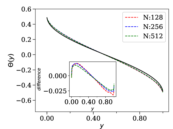
A comparison of the above equation with the microscopic simulation of the system Eq. (2) in Fig. (1) shows a very good agreement. The systematic differences are due to finite size effects, as was already noted in [11]. We next consider the steady state current. First, we observe that the fractional Laplacian 𝕃κ¯subscript𝕃¯𝜅\mathbb{L}_{\bar{\kappa}} can be expressed in the form of a divergence, namely in the form 𝕃κ¯=κ¯y𝔸subscript𝕃¯𝜅¯𝜅subscript𝑦𝔸\mathbb{L}_{\bar{\kappa}}=\bar{\kappa}\partial_{y}\mathbb{A} where the operator 𝔸𝔸\mathbb{A} is defined through the following action on Neumann basis vectors

𝔸ϕn(y)=λn1/4αn(y).𝔸subscriptitalic-ϕ𝑛𝑦superscriptsubscript𝜆𝑛14subscript𝛼𝑛𝑦\displaystyle\mathbb{A}\phi_{n}(y)=\lambda_{n}^{1/4}\alpha_{n}(y)~{}. (16)

We then see that (10) is in the form of a continuity equation τT(y,τ)=yj(y,τ)subscript𝜏𝑇𝑦𝜏subscript𝑦𝑗𝑦𝜏\partial_{\tau}T(y,\tau)=-\partial_{y}j(y,\tau) with the non-local energy current defined as j(y,τ)=κ¯𝔸T(y,τ)𝑗𝑦𝜏¯𝜅𝔸𝑇𝑦𝜏j(y,\tau)=\bar{\kappa}\mathbb{A}T(y,\tau). Using this definition of the current and the steady state temperature profile in (15) we immediately get the steady state current as

jδT=κ¯𝔸Tss(y)δT=κ¯c22,𝑗𝛿𝑇¯𝜅𝔸subscript𝑇𝑠𝑠𝑦𝛿𝑇¯𝜅𝑐22\displaystyle\frac{j}{\delta T}=\frac{\bar{\kappa}\mathbb{A}T_{ss}(y)}{\delta T}=\frac{\bar{\kappa}c}{2\sqrt{2}}~{}, (17)

where we used the identity noddαn(y)/λn1/2=1/(22)subscript𝑛oddsubscript𝛼𝑛𝑦superscriptsubscript𝜆𝑛12122\sum_{n\in{\rm odd}}\alpha_{n}(y)/\lambda_{n}^{1/2}=1/(2\sqrt{2}) (C). Note that this gives us the scaled current while the actual current is given by J=j/N𝐽𝑗𝑁J=j/\sqrt{N}, in agreement with results obtained in [11].
Refer to caption
Figure 1: Temperature profile from Eq. (15)(solid black line) compared with direct numerical simulations of microscopic system for system sizes N=128,256,512𝑁128256512N=128,256,512. In the inset the difference between Eq. (15) and numerical simulations is plotted for various system size.

3 Time evolution of temperature profile

The fractional Laplacian equation (10) allow us to study the time evolution of the temperature profile, starting from given initial and boundary conditions, and the eventual approach to the steady state at large times. Here we address the problem of describing the system’s time evolution. As before, the temperature profile at any time τ𝜏\tau in the form T(y,τ)=Tss(y)+f(y,τ)𝑇𝑦𝜏subscript𝑇𝑠𝑠𝑦𝑓𝑦𝜏T(y,\tau)=T_{ss}(y)+f(y,\tau), where again f(y,τ)𝑓𝑦𝜏f(y,\tau) satisfies Eq. (10) but with vanishing Dirichlet boundary conditions, f(0,τ)=f(1,τ)=0𝑓0𝜏𝑓1𝜏0f(0,\tau)=f(1,\tau)=0. Let {ψn}subscript𝜓𝑛\{\psi_{n}\} be the eigenvectors with corresponding eigenvalues μ1<μ2<μ3subscript𝜇1subscript𝜇2subscript𝜇3\mu_{1}<\mu_{2}<\mu_{3}\dots of 𝕃𝕃\mathbb{L} , satisfying the equation

𝕃ψn(y)=μnψn(y)𝕃subscript𝜓𝑛𝑦subscript𝜇𝑛subscript𝜓𝑛𝑦\displaystyle\mathbb{L}\psi_{n}(y)=\mu_{n}\psi_{n}(y) (18)

and boundary conditions ψn(0)=ψn(1)=0subscript𝜓𝑛0subscript𝜓𝑛10\psi_{n}(0)=\psi_{n}(1)=0. It can be shown that the operator 𝕃𝕃\mathbb{L} has a non-degenerate and positive spectrum (see below). We can then immediately write the solution for f(y,τ)𝑓𝑦𝜏f(y,\tau) as

f(y,τ)=n=1f^n(0)eκ¯μnτψn(y),𝑓𝑦𝜏subscript𝑛1subscript^𝑓𝑛0superscript𝑒¯𝜅subscript𝜇𝑛𝜏subscript𝜓𝑛𝑦\displaystyle f(y,\tau)=\sum_{n=1}\hat{f}_{n}(0)e^{-\bar{\kappa}\mu_{n}\tau}\psi_{n}(y), (19)
wheref^n(0)=01𝑑yf(y,0)ψn(y),wheresubscript^𝑓𝑛0superscriptsubscript01differential-d𝑦𝑓𝑦0subscript𝜓𝑛𝑦\displaystyle~{}{\rm where}~{}~{}\hat{f}_{n}(0)=\int_{0}^{1}dy~{}f(y,0)\psi_{n}(y),

are “fractional-Fourier coefficients” for the initial field f(y,0)𝑓𝑦0f(y,0). In the first section we outlined the procedure followed in [12] to find the Dirichlet eigenfunctions expanding the eigenfunctions ψnsubscript𝜓𝑛\psi_{n} in the orthogonal basis of {αl}l1subscriptsubscript𝛼𝑙𝑙1\{\alpha_{l}\}_{l\geq 1} as ψn(y)=l1ξnlαl(y)subscript𝜓𝑛𝑦subscript𝑙1subscript𝜉𝑛𝑙subscript𝛼𝑙𝑦\psi_{n}(y)=\sum_{l\geq 1}\xi_{nl}\alpha_{l}(y). We show here that much simplification and better accuracy is achieved if one expands ψnsubscript𝜓𝑛\psi_{n} directly in the Neumann basis {ϕm}m0subscriptsubscriptitalic-ϕ𝑚𝑚0\{\phi_{m}\}_{m\geq 0}.

ψ(y)=mχ^mϕm(y).𝜓𝑦subscript𝑚subscript^𝜒𝑚subscriptitalic-ϕ𝑚𝑦\displaystyle{\psi}(y)=\sum_{m}\hat{\chi}_{m}{\phi_{m}}(y). (20)

From Eq. (18), and using the definition of 𝕃𝕃\mathbb{L} in Eq. (9), we have

m0(μλm3/4)χ^mϕm(y)=0.subscript𝑚0𝜇superscriptsubscript𝜆𝑚34subscript^𝜒𝑚subscriptitalic-ϕ𝑚𝑦0\displaystyle\sum_{m\geq 0}(\mu-\lambda_{m}^{3/4})\hat{\chi}_{m}{\phi_{m}}(y)=0. (21)

There are two sets of solution for this equation. The first set is given by

χ^0=b2μ,χ^2k=bλ2k3/4μ,k1,χ^2k+1=0,k0,formulae-sequencesubscript^𝜒0𝑏2𝜇formulae-sequencesubscript^𝜒2𝑘𝑏superscriptsubscript𝜆2𝑘34𝜇formulae-sequence𝑘1formulae-sequencesubscript^𝜒2𝑘10𝑘0\displaystyle\hat{\chi}_{0}=-\frac{b}{\sqrt{2}\mu},~{}\hat{\chi}_{2k}=\frac{b}{\lambda_{2k}^{3/4}-\mu},~{}~{}k\geq 1,~{}~{}\hat{\chi}_{2k+1}=0,~{}~{}k\geq 0~{}, (22)

where we have made use of the identity m=1ϕ2m(x)=1/2superscriptsubscript𝑚1subscriptitalic-ϕ2𝑚𝑥12\sum_{m=1}^{\infty}\phi_{2m}(x)=-1/\sqrt{2}. The second solution set is given by

χ^2k+1=bλ2k+13/4μ,k0,χ^2k=0,k0,formulae-sequencesubscript^𝜒2𝑘1𝑏superscriptsubscript𝜆2𝑘134𝜇formulae-sequence𝑘0formulae-sequencesubscript^𝜒2𝑘0𝑘0\displaystyle\hat{\chi}_{2k+1}=\frac{b}{\lambda_{2k+1}^{3/4}-\mu},~{}~{}k\geq 0,~{}~{}~{}\hat{\chi}_{2k}=0,~{}~{}k\geq 0, (23)

where we have used the identity m=0ϕ2m+1(y)=0superscriptsubscript𝑚0subscriptitalic-ϕ2𝑚1𝑦0\sum_{m=0}^{\infty}\phi_{2m+1}(y)=0 (C). So far, b𝑏b and μ𝜇\mu are un-determined. We now use the Dirichlet boundary condition ψ(0)=χ^0+2k1χ^2k+k0χ^2k+1=0𝜓0subscript^𝜒02subscript𝑘1subscript^𝜒2𝑘subscript𝑘0subscript^𝜒2𝑘10\psi(0)=\hat{\chi}_{0}+\sqrt{2}\sum_{k\geq 1}\hat{\chi}_{2k}+\sum_{k\geq 0}\hat{\chi}_{2k+1}=0. From our first solution set Eq. (22) we then get the following equation satisfied by μ𝜇\mu

k11λ2k3/4μ=12μ.subscript𝑘11superscriptsubscript𝜆2𝑘34𝜇12𝜇\displaystyle\sum_{k\geq 1}\frac{1}{\lambda_{2k}^{3/4}-\mu}=\frac{1}{2\mu}~{}. (24)

Similarly, from the second solution set Eq. (23), we get

k01λ2k+13/4μ=0.subscript𝑘01superscriptsubscript𝜆2𝑘134𝜇0\displaystyle\sum_{k\geq 0}\frac{1}{\lambda_{2k+1}^{3/4}-\mu}=0~{}. (25)

The solution of either of the above two equations gives us the required eigenvalue, while Eqs. (22)-(23) provide us with the corresponding eigenfunction, with the constant b𝑏b fixed by normalization. We label the first set of solutions by μ2n+1,ψ2n+1subscript𝜇2𝑛1subscript𝜓2𝑛1\mu_{2n+1},\psi_{2n+1}, n0𝑛0n\geq 0 and the second set by μ2n,ψ2n+2subscript𝜇2𝑛subscript𝜓2𝑛2\mu_{2n},\psi_{2n+2}, n0𝑛0n\geq 0. From the structure of the eigenvalue equations it is clear that the roots are ordered set of numbers such that λ2n3/4<μ2n+1<λ2n+23/4superscriptsubscript𝜆2𝑛34subscript𝜇2𝑛1superscriptsubscript𝜆2𝑛234\lambda_{2n}^{3/4}<\mu_{2n+1}<\lambda_{2n+2}^{3/4} and λ2n13/4<μ2n<λ2n+13/4superscriptsubscript𝜆2𝑛134subscript𝜇2𝑛superscriptsubscript𝜆2𝑛134\lambda_{2n-1}^{3/4}<\mu_{2n}<\lambda_{2n+1}^{3/4}. Finally, introducing the notation, f|g=01𝑑xf(x)g(x)inner-product𝑓𝑔superscriptsubscript01differential-dsuperscript𝑥𝑓superscript𝑥𝑔superscript𝑥\langle f|g\rangle=\int_{0}^{1}dx^{\prime}f(x^{\prime})g(x^{\prime}), such that x|ψn=01𝑑xδ(xx)ψn(x)=ψn(x)inner-product𝑥subscript𝜓𝑛superscriptsubscript01differential-d𝑥𝛿𝑥superscript𝑥subscript𝜓𝑛superscript𝑥subscript𝜓𝑛𝑥\langle x|\psi_{n}\rangle=\int_{0}^{1}dx\delta(x-x^{\prime})\psi_{n}(x^{\prime})=\psi_{n}(x), the eigenvectors can now be written explicitly as

|ψ2n+1ketsubscript𝜓2𝑛1\displaystyle|\;\psi_{2n+1}\;\rangle =D2n+1(12μ2n+1|ϕ0+m11λ2m3/4μ2n+1|ϕ2m),absentsubscript𝐷2𝑛112subscript𝜇2𝑛1ketsubscriptitalic-ϕ0subscript𝑚11superscriptsubscript𝜆2𝑚34subscript𝜇2𝑛1ketsubscriptitalic-ϕ2𝑚\displaystyle=D_{2n+1}\left(-\frac{1}{\sqrt{2}\mu_{2n+1}}|\;\phi_{0}\;\rangle+\sum_{m\geq 1}\frac{1}{\lambda_{2m}^{3/4}-\mu_{2n+1}}|\;\phi_{2m}\;\rangle\right), (26)
|ψ2n+2ketsubscript𝜓2𝑛2\displaystyle|\;\psi_{2n+2}\;\rangle =D2n+2(m01λ2m+13/4μ2n+2|ϕ2m+1),absentsubscript𝐷2𝑛2subscript𝑚01superscriptsubscript𝜆2𝑚134subscript𝜇2𝑛2ketsubscriptitalic-ϕ2𝑚1\displaystyle=D_{2n+2}\left(\sum_{m\geq 0}\frac{1}{\lambda_{2m+1}^{3/4}-\mu_{2n+2}}|\;\phi_{2m+1}\;\rangle\right), (27)

where Dnsubscript𝐷𝑛D_{n}, found from the normalizing condition ψn|ψn=1inner-productsubscript𝜓𝑛subscript𝜓𝑛1\langle\psi_{n}|\psi_{n}\rangle=1, is explicitly given as,

D2n+1subscript𝐷2𝑛1\displaystyle D_{2n+1} =[12μ2n+12+m11(λ2m3/4μ2n+1)2]1/2,absentsuperscriptdelimited-[]12subscriptsuperscript𝜇22𝑛1subscript𝑚11superscriptsuperscriptsubscript𝜆2𝑚34subscript𝜇2𝑛1212\displaystyle=\left[\frac{1}{2\mu^{2}_{2n+1}}+\sum_{m\geq 1}\frac{1}{(\lambda_{2m}^{3/4}-\mu_{2n+1})^{2}}\right]^{-1/2},
D2n+2subscript𝐷2𝑛2\displaystyle D_{2n+2} =[m01(λ2m+13/4μ2n+2)2]1/2.absentsuperscriptdelimited-[]subscript𝑚01superscriptsuperscriptsubscript𝜆2𝑚134subscript𝜇2𝑛2212\displaystyle=\left[\sum_{m\geq 0}\frac{1}{(\lambda_{2m+1}^{3/4}-\mu_{2n+2})^{2}}\right]^{-1/2}~{}. (28)

Thus, as promised, we have managed to obtain a much efficient method for computing the Dirichlet spectrum of the fractional operator 𝕃𝕃\mathbb{L}. The roots of the eigenvalue equations (24)-(25) are solved numerically using Newton-Raphson method scanning in between these intervals. This procedure gives a fast and efficient way to compute the eigenvector while avoiding diagonalizing infinite dimensional matrices. For large k𝑘k, we have, μkλk3/4subscript𝜇𝑘superscriptsubscript𝜆𝑘34\mu_{k}\approx\lambda_{k}^{3/4}.

This procedure can be generalized to a fractional operator defined through the equation

𝕃(β)ϕn(y)=λnβϕn(y),superscript𝕃𝛽subscriptitalic-ϕ𝑛𝑦superscriptsubscript𝜆𝑛𝛽subscriptitalic-ϕ𝑛𝑦\displaystyle\mathbb{L}^{(\beta)}\phi_{n}(y)=\lambda_{n}^{\beta}\phi_{n}(y), (29)

for arbitrary β𝛽\beta. For diffusive case (β=1𝛽1\beta=1) one can obtain exact results and recover the expected result μk(β=1)=π2k2subscriptsuperscript𝜇𝛽1𝑘superscript𝜋2superscript𝑘2\mu^{(\beta=1)}_{k}=\pi^{2}k^{2} and ψk(y)=αk(y)subscript𝜓𝑘𝑦subscript𝛼𝑘𝑦\psi_{k}(y)=\alpha_{k}(y).

3.1 Properties of Dirichlet eigensystem of the fractional operator in bounded domain
Refer to caption
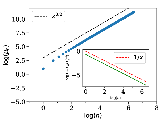
Figure 2: Eigenvalues computed from Eq. (24) and (25) plotted (blue dots) in log-log scale. Number of basis state used to approximate the function is 600600600. For large n𝑛n, μn(nπ)3/2similar-tosubscript𝜇𝑛superscript𝑛𝜋32\mu_{n}\sim(n\pi)^{3/2}, i.e. the Dirichlet and Neumann eigenvalues are same. For small n𝑛n there is a systematic difference between the two. A straight line of exponent x3/2superscript𝑥32x^{3/2} (black dot) is plotted alongside. In the inset we plot, log(1μn/λn3/4)1subscript𝜇𝑛superscriptsubscript𝜆𝑛34\log(1-\mu_{n}/\lambda_{n}^{3/4}) vs log(n)𝑛\log(n), which characterizes the difference between the Dirichlet and Neumann boundary eigenvalues. For large n𝑛n the value of this function goes to zero with slope 111, suggesting he difference between the two decreases linearly with n𝑛n. The red dashed line shows that it decays with an inverse power law of exponent 111.
Refer to caption
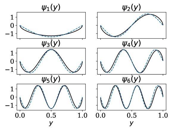
Figure 3: The first six eigenvectors of fractional operator, ψn(y)subscript𝜓𝑛𝑦\psi_{n}(y), (black) as compared to corresponding eigenfunctions of Laplacian i.e. sin\sin functions (blue dotted). The eigenstates are different from corresponding sin\sin functions near the boundaries even for large n𝑛n. These eigenfunctions are computed by summing over 600600600 basis states.

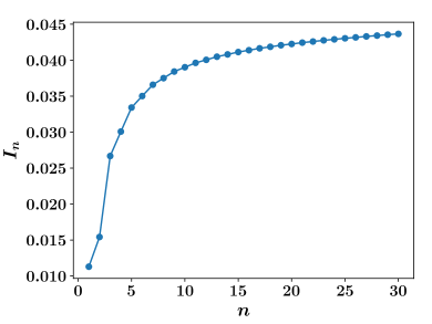
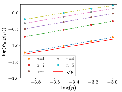
The numerical values of the computed eigenvalues are plotted in Fig. (2) in log-log scale, where we find that for large n𝑛n μn(nπ)3/2subscript𝜇𝑛superscript𝑛𝜋32\mu_{n}\approx(n\pi)^{3/2}, while for smaller values n𝑛n, there is a systematic deviation from the scaling due to the fact we are now working in a bounded domain. The first three eigenvalues (μnsubscript𝜇𝑛\mu_{n}) are approximately μ12.75,μ212.02,μ324.22formulae-sequencesubscript𝜇12.75formulae-sequencesubscript𝜇212.02subscript𝜇324.22\mu_{1}\approx 2.75,\mu_{2}\approx 12.02,\mu_{3}\approx 24.22. The first eigenvalue we have |μ1π3/2|/π3/20.5046subscript𝜇1superscript𝜋32superscript𝜋320.5046|\mu_{1}-\pi^{3/2}|/\pi^{3/2}\approx 0.5046 (see inset in Fig. (2)). This eigenvalue spectrum is expected to be identical to that in [12], upto a constant factor (see discussion in previous section). The first few numerically computed eigenvectors are shown in Fig. (3). The eigenvectors are similar to sin\sin functions but have divergent derivatives near the left and right boundaries. In order to compare it with corresponding sin\sin functions, we plot in Fig. (4) the overlap of integral between ψn(y)subscript𝜓𝑛𝑦\psi_{n}(y) and 2sin(nπy)2𝑛𝜋𝑦\sqrt{2}\sin(n\pi y) defined as In=101ψn(y)2sin(nπy)𝑑ysubscript𝐼𝑛1superscriptsubscript01subscript𝜓𝑛𝑦2𝑛𝜋𝑦differential-d𝑦I_{n}=1-\int_{0}^{1}\psi_{n}(y)\sqrt{2}\sin(n\pi y)~{}dy. This increases and saturates to a particular value, suggesting that the wave functions are quite different from sin\sin functions even for large n𝑛n. Also the eigenfunctions show a non-analytic behavior at the boundaries, for example near the left boundary one finds limy0+ψn(y)ysimilar-tosubscript𝑦superscript0subscript𝜓𝑛𝑦𝑦\lim_{y\to 0^{+}}\psi_{n}(y)\sim\sqrt{y} (see Fig. 4b), in contrast to sin\sin-functions for which limy0+sin(nπy)ysimilar-tosubscript𝑦superscript0𝑛𝜋𝑦𝑦\lim_{y\to 0^{+}}\sin(n\pi y)\sim y.

Refer to caption
Refer to caption
Figure 4: (a)(Left) To quantify the similarity between ψn(y)subscript𝜓𝑛𝑦\psi_{n}(y) and 2sin(nπy)2𝑛𝜋𝑦\sqrt{2}\sin(n\pi y), we plot the overlap integral, In=101ψn(y)2sin(nπy)𝑑ysubscript𝐼𝑛1superscriptsubscript01subscript𝜓𝑛𝑦2𝑛𝜋𝑦differential-d𝑦I_{n}=1-\int_{0}^{1}\psi_{n}(y)\sqrt{2}\sin(n\pi y)~{}dy . For large n𝑛n this seems to be saturating to a finite value, suggesting that the eigenfunctions ψnsubscript𝜓𝑛\psi_{n} are quite different from sin\sin functions. (b)(right) Scaling at boundaries of the eigenvectors in log-log scale shows that at the boundaries, the wave-function scales as y𝑦\sqrt{y}.

The eigenspectrum of fractional operator in bounded domain has been discussed earlier in the literature, using somewhat phenomenological approaches [18, 23, 24, 25]. It is not clear if those approaches can be related to that presented in this paper.
3.2 Comparison of time evolution formula with numerical simulations of the HCME model

We now compare the prediction from Eq. (19), with κ¯=1/(22)¯𝜅122\bar{\kappa}=1/(2\sqrt{2}), with results from direct microscopic simulations, described by Eq. (2) with the additional stochastic exchange dynamics. Initially the system of size N𝑁N is prepared in a step initial condition, given by

Tisubscript𝑇𝑖\displaystyle T_{i} =TL,1i<N/2,formulae-sequenceabsentsubscript𝑇𝐿1𝑖𝑁2\displaystyle=T_{L},~{}1\leq i<N/2,
=TR,N/2iN+1.formulae-sequenceabsentsubscript𝑇𝑅𝑁2𝑖𝑁1\displaystyle=T_{R},~{}N/2\leq i\leq N+1. (30)

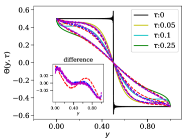
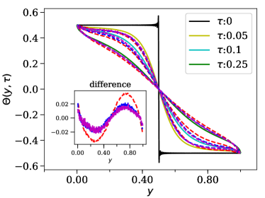
At large times it reaches a steady state described by Eq. (15). At various intermediate times, we plot the function Θ(y,τ)=T(y,τ)T¯=Tss(y)+f(y,τ)T¯Θ𝑦𝜏𝑇𝑦𝜏¯𝑇subscript𝑇𝑠𝑠𝑦𝑓𝑦𝜏¯𝑇\Theta(y,\tau)=T(y,\tau)-\overline{T}=T_{ss}(y)+f(y,\tau)-\overline{T}, such that Θ(0,τ)=1/2=Θ(1,τ)Θ0𝜏12Θ1𝜏\Theta(0,\tau)=1/2=-\Theta(1,\tau). In Fig. (5) we show the temperature profile at intermediate times from microscopic simulation with scaled space (y=i/N𝑦𝑖𝑁y=i/N) and times (τ=t/N3/2𝜏𝑡superscript𝑁32\tau=t/N^{3/2}) for various system sizes. We note that with increasing system size, the data converges to the prediction from Eq. (19). The difference between the numerical profiles and the predicted theoretical profile is shown in the inset. As we increase the system size, this difference systematically decreases. We also demonstrate that using standard Dirichlet sin\sin-functions, instead of the ψ𝜓\psi-functions, leads to significant differences, especially near the boundaries.
Refer to caption
Refer to caption
Figure 5: The time evolution of temperature starting from an initial step profile. The function Θ(y,τ)=T(y,τ)T¯=Tss(y)+f(y,τ)T¯Θ𝑦𝜏𝑇𝑦𝜏¯𝑇subscript𝑇𝑠𝑠𝑦𝑓𝑦𝜏¯𝑇\Theta(y,\tau)=T(y,\tau)-\overline{T}=T_{ss}(y)+f(y,\tau)-\overline{T} is plotted and compared with numerical simulations. In the left figure, dashed lines indicate simulation results for the time-evolution, for system sizes N=128𝑁128N=128 (red), N=256𝑁256N=256 (blue), N=512𝑁512N=512 (magenta). The solid lines at different scaled times (τ𝜏\tau) are generated from Eq. (19) by summing over 600600600 basis states. (right) The same, but now with the theoretical curves computed using the sin\sin-functions instead of the ψ𝜓\psi-functions, and eigenvalues λn3/4superscriptsubscript𝜆𝑛34\lambda_{n}^{3/4} instead of μnsubscript𝜇𝑛\mu_{n}. We notice that they do not match well with simulations, specially the deviations are prominent near the two boundary.

4 Adding noise satisfying fluctuation dissipation to describe equilibrium fluctuations in finite system

In [21], the harmonic chain with random momentum flips (HCMF model) was studied. In the HCMF, the stochastic dynamics flips the momentum of the particle and is embedded in the Hamiltonian dynamics such that the macroscopic dynamics is diffusive. It was shown that the equilibrium energy fluctuations e(x,t)=E(x,t)E(x,t)𝑒𝑥𝑡𝐸𝑥𝑡delimited-⟨⟩𝐸𝑥𝑡e(x,t)=E(x,t)-\langle E(x,t)\rangle, where E(x,t)𝐸𝑥𝑡E(x,t) is the local energy of the system at time t𝑡t, satisfies the noisy diffusion equation te(x,t)=x2e(x,t)+x(DT(x,t)η(x,t))subscript𝑡𝑒𝑥𝑡superscriptsubscript𝑥2𝑒𝑥𝑡subscript𝑥𝐷𝑇𝑥𝑡𝜂𝑥𝑡\partial_{t}e(x,t)=\partial_{x}^{2}e(x,t)+\partial_{x}(DT(x,t)\eta(x,t)), with η𝜂\eta a space-time mean zero white noise. As a note of caution, from here onwards, we use a different notation than that of the previous sections with {x,y}[0,1]𝑥𝑦01\{x,y\}\in[0,1], and t𝑡t is, in general, referred to a scaled time. The aim of this section is to establish a fractional fluctuating equation for the HCME model, which has anomalous diffusion properties. Using this equation, we establish a Green-Kubo formula relating the equilibrium current fluctuations to the non-equilibrium current. Next, we discuss the long-range correlations and conjecture a form for the long-range correlations of energy and test it using simulations.

The generalized equation, which we hypothesize in equilibrium at temperature T𝑇T is

t|etsubscript𝑡ketsubscript𝑒𝑡\displaystyle\partial_{t}|\;e_{t}\;\rangle =𝕃κ¯|et+2κ¯(BT|ηt),absentsubscript𝕃¯𝜅ketsubscript𝑒𝑡2¯𝜅𝐵𝑇ketsubscript𝜂𝑡\displaystyle=-\mathbb{L}_{\bar{\kappa}}|\;e_{t}\;\rangle+\sqrt{2\bar{\kappa}}\nabla(BT|\;\eta_{t}\;\rangle), (31)

where η(x,t)𝜂𝑥𝑡\eta(x,t) is a white Gaussian noise with η(x)=0delimited-⟨⟩𝜂𝑥0\big{\langle}\eta(x)\big{\rangle}=0, η(x,t)η(y,t)=δ(xy)δ(tt)delimited-⟨⟩𝜂𝑥𝑡𝜂𝑦superscript𝑡𝛿𝑥𝑦𝛿𝑡superscript𝑡\big{\langle}\eta(x,t)\eta(y,t^{\prime})\big{\rangle}=\delta(x-y)\delta(t-t^{\prime}) and 𝕃κ¯subscript𝕃¯𝜅\mathbb{L}_{\bar{\kappa}} is the fractional Laplacian as defined in Eq. (10). The explicit form for the operator BB𝐵superscript𝐵BB^{\dagger} is established through the requirement that energy fluctuations must respect the fluctuation dissipation (FD) in equilibrium. We define the Green function satisfying

tGt=𝕃κ¯Gt,x|G0|x=G0xx=δ(xx),formulae-sequencesubscript𝑡subscript𝐺𝑡subscript𝕃¯𝜅subscript𝐺𝑡quantum-operator-product𝑥subscript𝐺0superscript𝑥subscriptsuperscript𝐺𝑥superscript𝑥0𝛿𝑥superscript𝑥\displaystyle\partial_{t}G_{t}=-\mathbb{L}_{\bar{\kappa}}G_{t},~{}\langle x|G_{0}|x^{\prime}\rangle=G^{xx^{\prime}}_{0}=\delta(x-x^{\prime}), (32)

with Dirichlet boundary conditions in x[0,1]𝑥01x\in[0,1]. This can then be easily expressed in terms of the basis states {ψn}n1subscriptsubscript𝜓𝑛𝑛1\{\psi_{n}\}_{n\geq 1} as Gtxx=n=1ψn(x)ψn(x)eκ¯μntsubscriptsuperscript𝐺𝑥superscript𝑥𝑡subscript𝑛1subscript𝜓𝑛𝑥subscript𝜓𝑛superscript𝑥superscript𝑒¯𝜅subscript𝜇𝑛𝑡G^{xx^{\prime}}_{t}=\sum_{n=1}\psi_{n}(x)\psi_{n}(x^{\prime})e^{-\bar{\kappa}\mu_{n}t}. The long-time solution to Eq. (31) is then given by

e(x,t)=𝑒𝑥𝑡absent\displaystyle e(x,t)= 2κ¯t𝑑sx|Gts|(BTηs),2¯𝜅superscriptsubscript𝑡differential-d𝑠quantum-operator-product𝑥subscript𝐺𝑡𝑠𝐵𝑇subscript𝜂𝑠\displaystyle\sqrt{2\bar{\kappa}}\int_{-\infty}^{t}ds\langle\;x\;|\;G_{t-s}\;|\;\nabla(BT\eta_{s})\;\rangle,
=\displaystyle= 2κ¯t𝑑sx|Gts|(BTηs).2¯𝜅superscriptsubscript𝑡differential-d𝑠quantum-operator-product𝑥subscript𝐺𝑡𝑠𝐵𝑇subscript𝜂𝑠\displaystyle-\sqrt{2\bar{\kappa}}\int_{-\infty}^{t}ds\langle\;x\;|\;\nabla G_{t-s}\;|\;(BT\eta_{s})\;\rangle. (33)

The equal time correlation function in equilibrium defined as Ceq(x,y)=e(x,t)e(y,t)subscript𝐶eq𝑥𝑦delimited-⟨⟩𝑒𝑥𝑡𝑒𝑦𝑡C_{\rm eq}(x,y)=\big{\langle}e(x,t)e(y,t)\big{\rangle} then is given as

Ceq(x,y)=subscript𝐶eq𝑥𝑦absent\displaystyle C_{\rm eq}(x,y)= 2κt𝑑st𝑑sx|Gts|BTηsηsTB|Gts|y,2𝜅superscriptsubscript𝑡differential-d𝑠superscriptsubscript𝑡differential-dsuperscript𝑠delimited-⟨⟩quantum-operator-product𝑥subscript𝐺𝑡𝑠𝐵𝑇subscript𝜂𝑠quantum-operator-productsubscript𝜂superscript𝑠𝑇superscript𝐵subscript𝐺𝑡superscript𝑠𝑦\displaystyle 2\kappa\int_{-\infty}^{t}ds~{}\int_{-\infty}^{t}ds^{\prime}\big{\langle}\langle\;x\;|\;\nabla G_{t-s}\;|\;BT\eta_{s}\;\rangle\langle\;\eta_{s^{\prime}}TB^{\dagger}\;|\;\nabla G_{t-s^{\prime}}\;|\;y\;\rangle\big{\rangle},
=\displaystyle= 2κ¯T2t𝑑sx|GtsBBGts|y,2¯𝜅superscript𝑇2superscriptsubscript𝑡differential-d𝑠quantum-operator-product𝑥subscript𝐺𝑡𝑠𝐵superscript𝐵subscript𝐺𝑡𝑠𝑦\displaystyle~{}2\bar{\kappa}T^{2}\int_{-\infty}^{t}ds~{}\langle\;x\;|\;\nabla G_{t-s}BB^{\dagger}\nabla G_{t-s}\;|\;y\;\rangle, (34)
=\displaystyle= 2κ¯T2t𝑑sx|GtsBBGts|y,2¯𝜅superscript𝑇2superscriptsubscript𝑡differential-d𝑠quantum-operator-product𝑥subscript𝐺𝑡𝑠𝐵superscript𝐵subscript𝐺𝑡𝑠𝑦\displaystyle-2\bar{\kappa}T^{2}\int_{-\infty}^{t}ds\langle\;x\;|\;G_{t-s}\nabla BB^{\dagger}\nabla G_{t-s}\;|\;y\;\rangle,

where the statistical average is used and we integrate out the space time white noise to give x|BηsηsB|y=Bη(s)Bη(s)=δ(ss)BB(x,y)delimited-⟨⟩delimited-⟨⟩conditionalsuperscript𝑥𝐵subscript𝜂𝑠delimited-⟨⟩conditionalsubscript𝜂superscript𝑠superscript𝐵superscript𝑦delimited-⟨⟩𝐵𝜂𝑠𝐵𝜂superscript𝑠𝛿𝑠superscript𝑠𝐵superscript𝐵superscript𝑥superscript𝑦\big{\langle}\langle x^{\prime}|B\eta_{s}\rangle\langle\eta_{s^{\prime}}B^{\dagger}|y^{\prime}\rangle\big{\rangle}=\big{\langle}{B\eta(s)}B\eta(s^{\prime})\big{\rangle}=\delta(s-s^{\prime})BB^{\dagger}(x^{\prime},y^{\prime}) followed by an integration by parts. Here, the big angles, delimited-⟨⟩\big{\langle}\dots\big{\rangle} denote average over space-time white noise profiles whereas ..|\langle..| and |..|..\rangle denote the bra-ket notation, e.g. x|e=e(x,t)inner-product𝑥𝑒𝑒𝑥𝑡\langle x|e\rangle=e(x,t). If we identify κ¯BB=𝕃κ¯¯𝜅𝐵superscript𝐵subscript𝕃¯𝜅-\bar{\kappa}\nabla BB^{\dagger}\nabla=\mathbb{L}_{\bar{\kappa}}, and using Eq. (32) we recover FD relation in equilibrium

Ceq(x,y)=subscript𝐶eq𝑥𝑦absent\displaystyle C_{\rm eq}(x,y)= T2t𝑑s(x|Gts𝕃κ¯Gts|y+y|Gts𝕃κ¯Gts|x),superscript𝑇2superscriptsubscript𝑡differential-d𝑠quantum-operator-product𝑥subscript𝐺𝑡𝑠subscript𝕃¯𝜅subscript𝐺𝑡𝑠𝑦quantum-operator-product𝑦subscript𝐺𝑡𝑠subscript𝕃¯𝜅subscript𝐺𝑡𝑠𝑥\displaystyle~{}T^{2}\int_{-\infty}^{t}ds~{}\left(\langle\;x\;|\;G_{t-s}\mathbb{L}_{\bar{\kappa}}G_{t-s}\;|\;y\;\rangle+\langle\;y\;|\;G_{t-s}\mathbb{L}_{\bar{\kappa}}G_{t-s}\;|\;x\;\rangle\right),
=\displaystyle= T2t𝑑ssx|GtsGts|y=T2δ(xy),superscript𝑇2superscriptsubscript𝑡differential-d𝑠subscript𝑠quantum-operator-product𝑥subscript𝐺𝑡𝑠subscript𝐺𝑡𝑠𝑦superscript𝑇2𝛿𝑥𝑦\displaystyle~{}T^{2}\int_{-\infty}^{t}ds~{}\partial_{s}\langle\;x\;|\;G_{t-s}G_{t-s}\;|\;y\;\rangle=~{}T^{2}\delta(x-y), (35)

where we used the fact that changing xy𝑥𝑦x\leftrightarrow y would not change the correlation function due to time reversal symmetry of the microscopic dynamics. The operator BB𝐵superscript𝐵BB^{\dagger} can consistently be defined on a function g(x)𝑔𝑥g(x), expanded in {αn}n1subscriptsubscript𝛼𝑛𝑛1\{\alpha_{n}\}_{n\geq 1} basis, as g(x)=ng^nαn(x)𝑔𝑥subscript𝑛subscript^𝑔𝑛subscript𝛼𝑛𝑥g(x)=\sum_{n}\hat{g}_{n}\alpha_{n}(x). Again, using the definition of 𝕃κ¯=κ¯BBsubscript𝕃¯𝜅¯𝜅𝐵superscript𝐵\mathbb{L}_{\bar{\kappa}}=-\bar{\kappa}\nabla BB^{\dagger}\nabla in Eq. (9), we define the symmetric operator BB𝐵superscript𝐵BB^{\dagger} as,

01𝑑xBB(x,x)g(x)=n=11(λn)1/4g^nαn(x).superscriptsubscript01differential-dsuperscript𝑥𝐵superscript𝐵𝑥superscript𝑥𝑔superscript𝑥superscriptsubscript𝑛11superscriptsubscript𝜆𝑛14subscript^𝑔𝑛subscript𝛼𝑛𝑥\displaystyle\int_{0}^{1}dx^{\prime}BB^{\dagger}(x,x^{\prime})g(x^{\prime})=\sum_{n=1}^{\infty}\frac{1}{(\lambda_{n})^{1/4}}\hat{g}_{n}\alpha_{n}(x). (36)

Note that we do not assume anything about the form of the operator B𝐵B, which would be important if we were to study non-equilibrium phenomena where temperature is not constant in space.

The connection between the 𝕃𝕃\mathbb{L} operator with the BB𝐵superscript𝐵BB^{\dagger} allows one to identify the current (through continuity equation) as

j(x,t)=κ¯01𝑑xBB(x,x)xe(x,t).𝑗𝑥𝑡¯𝜅superscriptsubscript01differential-dsuperscript𝑥𝐵superscript𝐵𝑥superscript𝑥subscriptsuperscript𝑥𝑒superscript𝑥𝑡j(x,t)=-\bar{\kappa}\int_{0}^{1}dx^{\prime}~{}BB^{\dagger}(x,x^{\prime})\partial_{x^{\prime}}e(x^{\prime},t).

Note that the above equation is a linear response relation, but in contrast to the diffusive case, this relation is non-local. Such non-local linear response relation have recently been reported in [20], where an alternate series representation of the kernel BB(x,x)𝐵superscript𝐵𝑥superscript𝑥BB^{\dagger}(x,x^{\prime}) has been provided for HCME model with general boundary conditions. In D, we show that the spectral representation in Eq. (36) is completely consistent with the series representation in [20] for fixed boundary condition.

4.1 Spatio-temporal equilibrium energy correlations

We compute the two time spatio-temporal energy correlations in equilibrium defined as Ceq(x,t,y,t)=e(x,t)e(y,t)subscript𝐶eq𝑥𝑡𝑦superscript𝑡delimited-⟨⟩𝑒𝑥𝑡𝑒𝑦superscript𝑡C_{\rm eq}(x,t,y,t^{\prime})=\big{\langle}e(x,t)e(y,t^{\prime})\big{\rangle} and show that at large times it is given in terms of the Green functions. The two time correlations can be analogously written down as,

Ceq(x,t,y,t)=subscript𝐶eq𝑥𝑡𝑦superscript𝑡absent\displaystyle C_{\rm eq}(x,t,y,t^{\prime})= 2κ¯t𝑑st𝑑sx|Gts|BTηsηsTB|Gts|y,2¯𝜅superscriptsubscript𝑡differential-d𝑠superscriptsubscriptsuperscript𝑡differential-dsuperscript𝑠delimited-⟨⟩quantum-operator-product𝑥subscript𝐺𝑡𝑠𝐵𝑇subscript𝜂𝑠quantum-operator-productsubscript𝜂superscript𝑠𝑇superscript𝐵subscript𝐺superscript𝑡superscript𝑠𝑦\displaystyle 2\bar{\kappa}\int_{-\infty}^{t}ds~{}\int_{-\infty}^{t^{\prime}}ds^{\prime}\big{\langle}\langle\;x\;|\;\nabla G_{t-s}\;|\;BT\eta_{s}\;\rangle\langle\;\eta_{s^{\prime}}TB^{\dagger}\;|\;\nabla G_{t^{\prime}-s^{\prime}}\;|\;y\;\rangle\big{\rangle}, (37)

Taking t>t𝑡superscript𝑡t>t^{\prime}, and performing the t𝑡t integral we have,

Ceq(x,t,y,t)=subscript𝐶eq𝑥𝑡𝑦superscript𝑡absent\displaystyle C_{\rm eq}(x,t,y,t^{\prime})= 2κ¯T2t𝑑sx|GtsBBGts|yθ(tt),2¯𝜅superscript𝑇2superscriptsubscriptsuperscript𝑡differential-d𝑠quantum-operator-product𝑥subscript𝐺𝑡𝑠𝐵superscript𝐵subscript𝐺superscript𝑡𝑠𝑦𝜃𝑡superscript𝑡\displaystyle~{}-2\bar{\kappa}T^{2}\int_{-\infty}^{t^{\prime}}ds~{}\langle\;x\;|\;G_{t-s}\nabla BB^{\dagger}\nabla G_{t^{\prime}-s}\;|\;y\;\rangle\theta(t-t^{\prime}),

where θ(t)𝜃𝑡\theta(t) is the Heaviside theta function. Proceeding as before and identifying κ¯BB=𝕃κ¯¯𝜅𝐵superscript𝐵subscript𝕃¯𝜅-\bar{\kappa}\nabla BB^{\dagger}\nabla=\mathbb{L}_{\bar{\kappa}} and interchanging x,y𝑥𝑦x,y

Ceq(x,t,y,t)=subscript𝐶eq𝑥𝑡𝑦superscript𝑡absent\displaystyle C_{\rm eq}(x,t,y,t^{\prime})= T2t𝑑s(x|Gts𝕃κ¯Gts|y+y|Gts𝕃κ¯Gts|x),superscript𝑇2superscriptsubscriptsuperscript𝑡differential-d𝑠quantum-operator-product𝑥subscript𝐺𝑡𝑠subscript𝕃¯𝜅subscript𝐺superscript𝑡𝑠𝑦quantum-operator-product𝑦subscript𝐺𝑡𝑠subscript𝕃¯𝜅subscript𝐺superscript𝑡𝑠𝑥\displaystyle~{}T^{2}\int_{-\infty}^{t^{\prime}}ds\left(\langle\;x\;|\;G_{t-s}\mathbb{L}_{\bar{\kappa}}G_{t^{\prime}-s}\;|\;y\;\rangle+\langle\;y\;|\;G_{t-s}\mathbb{L}_{\bar{\kappa}}G_{t^{\prime}-s}\;|\;x\;\rangle\right),
=\displaystyle= T2t𝑑ssx|GtsGts|y=T2Gttxyθ(tt).superscript𝑇2superscriptsubscriptsuperscript𝑡differential-d𝑠subscript𝑠quantum-operator-product𝑥subscript𝐺𝑡𝑠subscript𝐺superscript𝑡𝑠𝑦superscript𝑇2subscriptsuperscript𝐺𝑥𝑦𝑡superscript𝑡𝜃𝑡superscript𝑡\displaystyle~{}T^{2}\int_{-\infty}^{t^{\prime}}ds\partial_{s}\langle\;x\;|\;G_{t-s}G_{t^{\prime}-s}\;|\;y\;\rangle=~{}T^{2}G^{xy}_{t-t^{\prime}}\theta(t-t^{\prime}). (38)

Along with a similar term for t<t𝑡superscript𝑡t<t^{\prime}, we can write the two time correlations as,

Ceq(x,t,y,t)=x|T2Gttθ(tt)+T2Gttθ(tt)|y.subscript𝐶eq𝑥𝑡𝑦superscript𝑡quantum-operator-product𝑥superscript𝑇2subscript𝐺𝑡superscript𝑡𝜃𝑡superscript𝑡superscript𝑇2subscript𝐺superscript𝑡𝑡𝜃superscript𝑡𝑡𝑦\displaystyle C_{\rm eq}(x,t,y,t^{\prime})=\langle\;x\;|T^{2}G_{t-t^{\prime}}\theta(t-t^{\prime})+T^{2}G_{t^{\prime}-t}\theta(t^{\prime}-t)|\;y\;\rangle. (39)

4.2 Current fluctuations in equilibrium

Here we define the fluctuating current in the system and then establish Green-Kubo relation for the system connecting the equilibrium current fluctuations and non-equilibrium current in the system. We expect that since the total energy in the isolated system is conserved, the energy flow across the system must be in continuity form te(x,t)+xj(x,t)=0subscript𝑡𝑒𝑥𝑡subscript𝑥𝑗𝑥𝑡0\partial_{t}e(x,t)+\partial_{x}j(x,t)=0. Along with the definition of current in Eq. (16), the fluctuating current operator is defined as,

|jt=κ¯𝔸|et2κ¯|BTηt.ketsubscript𝑗𝑡¯𝜅𝔸ketsubscript𝑒𝑡2¯𝜅ket𝐵𝑇subscript𝜂𝑡\displaystyle|\;j_{t}\;\rangle=\bar{\kappa}\mathbb{A}|\;e_{t}\;\rangle-\sqrt{2\bar{\kappa}}|\;BT\eta_{t}\;\rangle. (40)

From previous section, it follows that the definition of current operator as 𝔸=BB𝔸𝐵superscript𝐵\mathbb{A}=-BB^{\dagger}\nabla. We also note that since the current operator is odd in derivatives, the adjoint current operator has the property, 𝔸=𝔸superscript𝔸𝔸\mathbb{A}^{\dagger}=-\mathbb{A}. Now we expect that [26] the second moment of equilibrium total current fluctuations is related to the current in NESS through the Green-Kubo formula. A precise statement is:

limτq2δT=02τT2=limδT0jδT,subscript𝜏subscriptdelimited-⟨⟩superscript𝑞2𝛿𝑇02𝜏superscript𝑇2subscript𝛿𝑇0𝑗𝛿𝑇\displaystyle\lim_{\tau\to\infty}\frac{\langle q^{2}\rangle_{\delta T=0}}{2\tau T^{2}}=\lim_{\delta T\to 0}\frac{j}{\delta T}, (41)

where q(τ)=0τ𝑑t01𝑑xj(x,t)𝑞𝜏superscriptsubscript0𝜏differential-d𝑡superscriptsubscript01differential-d𝑥𝑗𝑥𝑡q(\tau)=\int_{0}^{\tau}dt\int_{0}^{1}dxj(x,t). In order to verify this relation, we first express q2delimited-⟨⟩superscript𝑞2\langle q^{2}\rangle, in terms of the integrals of the unequal time current correlations:

q2δT=0τ=subscriptdelimited-⟨⟩superscript𝑞2𝛿𝑇0𝜏absent\displaystyle\frac{\langle q^{2}\rangle_{\delta T=0}}{\tau}= 1τ0τ𝑑t0τ𝑑t01𝑑x01𝑑yj(x,t)j(y,t).1𝜏superscriptsubscript0𝜏differential-d𝑡superscriptsubscript0𝜏differential-dsuperscript𝑡superscriptsubscript01differential-d𝑥superscriptsubscript01differential-d𝑦delimited-⟨⟩𝑗𝑥𝑡𝑗𝑦superscript𝑡\displaystyle\frac{1}{\tau}\int_{0}^{\tau}dt\int_{0}^{\tau}dt^{\prime}\int_{0}^{1}dx\int_{0}^{1}dy\big{\langle}j(x,t)j(y,t^{\prime})\big{\rangle}. (42)

Using Eq. (40) the current correlations can be split into four parts:

j(x,t)j(y,t)=delimited-⟨⟩𝑗𝑥𝑡𝑗𝑦superscript𝑡absent\displaystyle\big{\langle}j(x,t)j(y,t^{\prime})\big{\rangle}= κ¯2x|𝔸|etet|𝔸|yI+2κ¯T2x|BB|yIIδ(tt)subscriptsuperscript¯𝜅2delimited-⟨⟩quantum-operator-product𝑥𝔸subscript𝑒𝑡quantum-operator-productsubscript𝑒superscript𝑡superscript𝔸𝑦Isubscript2¯𝜅superscript𝑇2quantum-operator-product𝑥𝐵superscript𝐵𝑦II𝛿𝑡superscript𝑡\displaystyle\underbrace{\bar{\kappa}^{2}\big{\langle}\langle\;x\;|\mathbb{A}|\;e_{t}\;\rangle\langle\;e_{t^{\prime}}\;|\mathbb{A}^{\dagger}|\;y\;\rangle\big{\rangle}}_{\textup{I}}+\underbrace{2\bar{\kappa}T^{2}\langle\;x\;|\;BB^{\dagger}\;|\;y\;\rangle}_{\textup{II}}\delta(t-t^{\prime}) (43)
\displaystyle- 2κ¯3/2x|𝔸|etηtTB|yIII2κ¯3/2x|BTηtet|𝔸|yIV.subscript2superscript¯𝜅32delimited-⟨⟩delimited-⟨⟩𝑥𝔸subscript𝑒𝑡delimited-⟨⟩conditionalsubscript𝜂superscript𝑡𝑇superscript𝐵𝑦IIIsubscript2superscript¯𝜅32delimited-⟨⟩delimited-⟨⟩conditional𝑥𝐵𝑇subscript𝜂𝑡delimited-⟨⟩subscript𝑒superscript𝑡superscript𝔸𝑦IV\displaystyle\underbrace{\sqrt{2}\bar{\kappa}^{3/2}\big{\langle}\langle\;x\;|\;\mathbb{A}\;|\;e_{t}\;\rangle\langle\eta_{t^{\prime}}TB^{\dagger}|y\rangle\big{\rangle}}_{\textup{III}}-\underbrace{\sqrt{2}\bar{\kappa}^{3/2}\big{\langle}\langle x|BT\eta_{t}\rangle\langle\;e_{t^{\prime}}\;|\;\mathbb{A}^{\dagger}\;|\;y\;\rangle\big{\rangle}}_{\textup{IV}}.

Part III in the above equation can be simplified to

2κ¯3/2x|𝔸|etηtTB|y=2superscript¯𝜅32delimited-⟨⟩delimited-⟨⟩𝑥𝔸subscript𝑒𝑡delimited-⟨⟩conditionalsubscript𝜂superscript𝑡𝑇superscript𝐵𝑦absent\displaystyle\sqrt{2}\bar{\kappa}^{3/2}\big{\langle}\langle\;x\;|\;\mathbb{A}\;|\;e_{t}\;\rangle\langle\eta_{t^{\prime}}TB^{\dagger}|y\rangle\big{\rangle}= 2κ¯2t𝑑sx|𝔸Gts|(BTηs)ηtTB|y,2superscript¯𝜅2superscriptsubscript𝑡differential-d𝑠delimited-⟨⟩delimited-⟨⟩𝑥𝔸subscript𝐺𝑡𝑠𝐵𝑇subscript𝜂𝑠delimited-⟨⟩conditionalsubscript𝜂superscript𝑡𝑇superscript𝐵𝑦\displaystyle~{}2\bar{\kappa}^{2}\int_{-\infty}^{t}ds\big{\langle}\langle\;x\;|\;\mathbb{A}G_{t-s}\;|\;\nabla(BT\eta_{s})\;\rangle\langle\eta_{t^{\prime}}TB^{\dagger}|y\rangle\big{\rangle},
=\displaystyle= T22κ¯2x|(𝔸Gtt)BB|yθ(tt),superscript𝑇22superscript¯𝜅2quantum-operator-product𝑥𝔸subscript𝐺𝑡superscript𝑡𝐵superscript𝐵𝑦𝜃𝑡superscript𝑡\displaystyle-T^{2}2\bar{\kappa}^{2}\langle\;x\;|\;(\mathbb{A}\nabla G_{t-t^{\prime}})BB^{\dagger}\;|\;y\;\rangle\theta(t-t^{\prime}),
=\displaystyle= T22κ¯2x|𝔸Gtt𝔸|yθ(tt).superscript𝑇22superscript¯𝜅2quantum-operator-product𝑥𝔸subscript𝐺𝑡superscript𝑡superscript𝔸𝑦𝜃𝑡superscript𝑡\displaystyle T^{2}2\bar{\kappa}^{2}\langle\;x\;|\mathbb{A}G_{t-t^{\prime}}\mathbb{A}^{\dagger}|\;y\;\rangle\theta(t-t^{\prime}). (44)

Similarly part IV is given by

2κ¯3/2x|BTηtet|𝔸|y=2superscript¯𝜅32delimited-⟨⟩delimited-⟨⟩conditional𝑥𝐵𝑇subscript𝜂𝑡delimited-⟨⟩subscript𝑒superscript𝑡superscript𝔸𝑦absent\displaystyle\sqrt{2}\bar{\kappa}^{3/2}\big{\langle}\langle x|BT\eta_{t}\rangle\langle\;e_{t^{\prime}}\;|\;\mathbb{A}^{\dagger}\;|\;y\;\rangle\big{\rangle}= 2κ¯2T2t𝑑sx|Bηtηs(B)|Gts𝔸|y,2superscript¯𝜅2superscript𝑇2superscriptsubscriptsuperscript𝑡differential-d𝑠delimited-⟨⟩delimited-⟨⟩conditional𝑥𝐵subscript𝜂𝑡delimited-⟨⟩subscript𝜂𝑠superscript𝐵subscript𝐺superscript𝑡𝑠superscript𝔸𝑦\displaystyle~{}2\bar{\kappa}^{2}T^{2}\int_{-\infty}^{t^{\prime}}ds\big{\langle}\langle x|B\eta_{t}\rangle\langle\;\eta_{s}(\nabla B)^{\dagger}\;|\;G_{t^{\prime}-s}\mathbb{A}^{\dagger}\;|\;y\;\rangle\big{\rangle},
=\displaystyle= T22κ¯2x|BBGtt𝔸|yθ(tt),superscript𝑇22superscript¯𝜅2quantum-operator-product𝑥𝐵superscript𝐵subscript𝐺superscript𝑡𝑡superscript𝔸𝑦𝜃superscript𝑡𝑡\displaystyle-T^{2}2\bar{\kappa}^{2}\langle\;x\;|\;BB^{\dagger}\nabla G_{t^{\prime}-t}\mathbb{A}^{\dagger}\;|\;y\;\rangle\theta(t^{\prime}-t),
=\displaystyle= T22κ¯2x|𝔸Gtt𝔸|yθ(tt),superscript𝑇22superscript¯𝜅2quantum-operator-product𝑥𝔸subscript𝐺superscript𝑡𝑡superscript𝔸𝑦𝜃superscript𝑡𝑡\displaystyle T^{2}2\bar{\kappa}^{2}\langle\;x\;|\;\mathbb{A}G_{t^{\prime}-t}\mathbb{A}^{\dagger}\;|\;y\;\rangle\theta(t^{\prime}-t),

while part I, on using (39), gives

κ¯2x|𝔸|etet|𝔸|y=T2κ¯2[x|𝔸Gtt𝔸θ(tt)+𝔸Gtt𝔸θ(tt)|y].superscript¯𝜅2delimited-⟨⟩quantum-operator-product𝑥𝔸subscript𝑒𝑡quantum-operator-productsubscript𝑒superscript𝑡superscript𝔸𝑦superscript𝑇2superscript¯𝜅2delimited-[]quantum-operator-product𝑥𝔸subscript𝐺𝑡superscript𝑡superscript𝔸𝜃𝑡superscript𝑡𝔸subscript𝐺superscript𝑡𝑡superscript𝔸𝜃superscript𝑡𝑡𝑦\displaystyle\bar{\kappa}^{2}\big{\langle}\langle\;x\;|\mathbb{A}|\;e_{t}\;\rangle\langle\;e_{t^{\prime}}\;|\mathbb{A}^{\dagger}|\;y\;\rangle\big{\rangle}=T^{2}\bar{\kappa}^{2}\left[\langle\;x\;|\mathbb{A}G_{t-t^{\prime}}\mathbb{A}^{\dagger}\theta(t-t^{\prime})+\mathbb{A}G_{t^{\prime}-t}\mathbb{A}^{\dagger}\theta(t^{\prime}-t)|\;y\;\rangle\right]. (45)

We see that III+IV=2IIIIIV2I\textup{III}+\textup{IV}=2\textup{I}. The first term explicitly gives,

I=Iabsent\displaystyle\textup{I}= κ¯201𝑑x01𝑑y𝔸(x,x)et(x)et(y)𝔸(y,y),superscript¯𝜅2superscriptsubscript01differential-dsuperscript𝑥superscriptsubscript01differential-dsuperscript𝑦𝔸𝑥superscript𝑥delimited-⟨⟩subscript𝑒𝑡superscript𝑥subscript𝑒superscript𝑡superscript𝑦superscript𝔸superscript𝑦𝑦\displaystyle\bar{\kappa}^{2}\int_{0}^{1}dx^{\prime}\int_{0}^{1}dy^{\prime}\mathbb{A}(x,x^{\prime})\big{\langle}e_{t}(x^{\prime})e_{t^{\prime}}(y^{\prime})\big{\rangle}\mathbb{A}^{\dagger}(y^{\prime},y),
=\displaystyle= κ¯2T201𝑑x01𝑑y𝔸(x,x)𝔸(y,y)G|tt|(x,y),superscript¯𝜅2superscript𝑇2superscriptsubscript01differential-dsuperscript𝑥superscriptsubscript01differential-dsuperscript𝑦𝔸𝑥superscript𝑥𝔸𝑦superscript𝑦subscript𝐺𝑡superscript𝑡superscript𝑥superscript𝑦\displaystyle\bar{\kappa}^{2}T^{2}\int_{0}^{1}dx^{\prime}\int_{0}^{1}dy^{\prime}\mathbb{A}(x,x^{\prime})\mathbb{A}(y,y^{\prime})G_{|t-t^{\prime}|}(x^{\prime},y^{\prime}),
=\displaystyle= κ¯2T2n,l,lχ^nlχ^nl(λlλl)1/4eκ¯μn|tt|αl(x)αl(y).superscript¯𝜅2superscript𝑇2subscript𝑛𝑙superscript𝑙subscript^𝜒𝑛𝑙subscript^𝜒𝑛superscript𝑙superscriptsubscript𝜆𝑙subscript𝜆superscript𝑙14superscript𝑒¯𝜅subscript𝜇𝑛𝑡superscript𝑡subscript𝛼𝑙𝑥subscript𝛼superscript𝑙𝑦\displaystyle\bar{\kappa}^{2}T^{2}\sum_{n,l,l^{\prime}}\hat{\chi}_{nl}\hat{\chi}_{nl^{\prime}}(\lambda_{l}\lambda_{l^{\prime}})^{1/4}e^{-\bar{\kappa}\mu_{n}|t-t^{\prime}|}\alpha_{l}(x)\alpha_{l^{\prime}}(y). (46)

Therefore, the contribution of the parts IIIIIV=IIIIIIVI\textup{I}-\textup{III}-\textup{IV}=-\textup{I} in (42) gives, after doing the space and time integrals:

0τ𝑑t0τ𝑑t01𝑑x01𝑑y(I)=16κ¯2T2nllodd1κ¯μn[τ+(eμnτ1)μn]χ^nlχ^nl(λlλl)1/4.superscriptsubscript0𝜏differential-dsuperscript𝑡superscriptsubscript0𝜏differential-d𝑡superscriptsubscript01differential-d𝑥superscriptsubscript01differential-d𝑦I16superscript¯𝜅2superscript𝑇2subscript𝑛subscript𝑙superscript𝑙𝑜𝑑𝑑1¯𝜅subscript𝜇𝑛delimited-[]𝜏superscript𝑒subscript𝜇𝑛𝜏1subscript𝜇𝑛subscript^𝜒𝑛𝑙subscript^𝜒𝑛superscript𝑙superscriptsubscript𝜆𝑙subscript𝜆superscript𝑙14\displaystyle\int_{0}^{\tau}dt^{\prime}\int_{0}^{\tau}dt\int_{0}^{1}dx\int_{0}^{1}dy~{}(-\textup{I})=-16\bar{\kappa}^{2}T^{2}\sum_{n}\sum_{ll^{\prime}\;odd}\frac{1}{\bar{\kappa}\mu_{n}}\left[\tau+\frac{(e^{-\mu_{n}\tau}-1)}{\mu_{n}}\right]\hat{\chi}_{nl}\hat{\chi}_{nl^{\prime}}(\lambda_{l}\lambda_{l^{\prime}})^{-1/4}. (47)

On using (36), the contribution of part II in (42) gives

0τ𝑑t0τ𝑑t01𝑑x01𝑑y(II)=superscriptsubscript0𝜏differential-dsuperscript𝑡superscriptsubscript0𝜏differential-d𝑡superscriptsubscript01differential-d𝑥superscriptsubscript01differential-d𝑦IIabsent\displaystyle\int_{0}^{\tau}dt^{\prime}\int_{0}^{\tau}dt\int_{0}^{1}dx\int_{0}^{1}dy(\textup{II})= 2κ¯T20τ𝑑t0τ𝑑t01𝑑x01𝑑yBB(x,y)δ(tt),2¯𝜅superscript𝑇2superscriptsubscript0𝜏differential-dsuperscript𝑡superscriptsubscript0𝜏differential-d𝑡superscriptsubscript01differential-d𝑥superscriptsubscript01differential-d𝑦𝐵superscript𝐵𝑥𝑦𝛿𝑡superscript𝑡\displaystyle 2\bar{\kappa}T^{2}\int_{0}^{\tau}dt^{\prime}\int_{0}^{\tau}dt\int_{0}^{1}dx\int_{0}^{1}dyBB^{\dagger}(x,y)\delta(t-t^{\prime}),
=\displaystyle= 2κ¯T2τ01𝑑x01𝑑ynαn(x)αn(y)λn1/4,2¯𝜅superscript𝑇2𝜏superscriptsubscript01differential-d𝑥superscriptsubscript01differential-d𝑦subscript𝑛subscript𝛼𝑛𝑥subscript𝛼𝑛𝑦superscriptsubscript𝜆𝑛14\displaystyle~{}2\bar{\kappa}T^{2}\tau\int_{0}^{1}dx\int_{0}^{1}dy\sum_{n}\frac{\alpha_{n}(x)\alpha_{n}(y)}{\lambda_{n}^{1/4}},
=\displaystyle= 16κ¯T2τnodd1λn5/4.16¯𝜅superscript𝑇2𝜏subscript𝑛𝑜𝑑𝑑1superscriptsubscript𝜆𝑛54\displaystyle 16\bar{\kappa}T^{2}\tau\sum_{n\;odd}\frac{1}{\lambda_{n}^{5/4}}. (48)

Combining the above results we finally have

limτq2δT=02τT2=κ¯(8nodd1λn5/4nllodd8μnχ^nlχ^nl(λlλl)1/4).subscript𝜏subscriptdelimited-⟨⟩superscript𝑞2𝛿𝑇02𝜏superscript𝑇2¯𝜅8subscript𝑛𝑜𝑑𝑑1superscriptsubscript𝜆𝑛54subscript𝑛subscript𝑙superscript𝑙𝑜𝑑𝑑8subscript𝜇𝑛subscript^𝜒𝑛𝑙subscript^𝜒𝑛superscript𝑙superscriptsubscript𝜆𝑙subscript𝜆superscript𝑙14\displaystyle\lim_{\tau\to\infty}\frac{\langle q^{2}\rangle_{\delta T=0}}{2\tau T^{2}}=\bar{\kappa}\left(8\sum_{n\;odd}\frac{1}{\lambda_{n}^{5/4}}-\sum_{n}\sum_{ll^{\prime}\;odd}\frac{8}{\mu_{n}}\frac{\hat{\chi}_{nl}\hat{\chi}_{nl^{\prime}}}{(\lambda_{l}\lambda_{l^{\prime}})^{1/4}}\right). (49)

The first summation yields 0.50500.50500.5050\ldots and the second yields 0.0931absent0.0931\approx 0.0931, hence we get

limτq2δT=02T2τ0.4119κ¯,subscript𝜏subscriptdelimited-⟨⟩superscript𝑞2𝛿𝑇02superscript𝑇2𝜏0.4119¯𝜅\displaystyle\lim_{\tau\to\infty}\frac{\langle q^{2}\rangle_{\delta T=0}}{2T^{2}\tau}\approx 0.4119\bar{\kappa}, (50)

which, up to numerical accuracy is consistent with the numerical value of steady state current (j/δT=0.4124κ¯𝑗𝛿𝑇0.4124¯𝜅j/\delta T=0.4124\bar{\kappa}) we found in (17), thus validating the Green-Kubo formula in (41).

Note that in order to get the expected scaling in system size N𝑁N, we need to put in the appropriate length scaling of the eigenvalues and eigenfunctions, for example λnλn/N2subscript𝜆𝑛subscript𝜆𝑛superscript𝑁2\lambda_{n}\to\lambda_{n}/N^{2} and μnμn/N3/2subscript𝜇𝑛subscript𝜇𝑛superscript𝑁32\mu_{n}\to\mu_{n}/N^{3/2}). We also need to consider the integrated current Q(τ)=0τ𝑑t0N𝑑xj(x,t)𝑄𝜏superscriptsubscript0𝜏differential-d𝑡superscriptsubscript0𝑁differential-d𝑥𝑗𝑥𝑡Q(\tau)=\int_{0}^{\tau}dt\int_{0}^{N}dxj(x,t) and then one gets limτQ2δT=02T2τ0.4119κ¯Nsubscript𝜏subscriptdelimited-⟨⟩superscript𝑄2𝛿𝑇02superscript𝑇2𝜏0.4119¯𝜅𝑁\lim_{\tau\to\infty}\frac{\langle Q^{2}\rangle_{\delta T=0}}{2T^{2}\tau}\approx\frac{0.4119\bar{\kappa}}{\sqrt{N}} and JδT=jNδT0.4124κ¯N𝐽𝛿𝑇𝑗𝑁𝛿𝑇0.4124¯𝜅𝑁\frac{J}{\delta T}=\frac{j}{\sqrt{N}\delta T}\approx\frac{0.4124\bar{\kappa}}{\sqrt{N}}.

Refer to caption
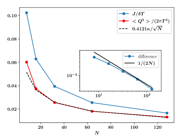
Figure 6: For the microscopic HCME model, we compute the two quantities, J/δT𝐽𝛿𝑇J/\delta T computed from non-equilibrium simulations connected to heat baths and <Q2>/(2τT2)expectationsuperscript𝑄22𝜏superscript𝑇2<Q^{2}>/(2\tau T^{2}) computed from equilibrium simulations, are plotted as a function of N𝑁N. The black dashed curve is for the theoretical current with appropriate scaling as given in Eq. (17). We find that for small N𝑁N, these two do not match, and the difference between the two decays as 1/N1𝑁1/N (inset), which is due to the contribution of current from the stochastic part. This signifies that at large N𝑁N, Green-Kubo holds while for small N𝑁N, it fails.

The above verification of the Green-Kubo identity was obtained using the fluctuating fractional diffusion equation, which is valid in the limit of large system size. A natural question is as to whether the identity is true even for a small chain with the microscopic dynamics (HCME), as would be expected from the fluctuation theorem. In Fig. (6), we present a numerical comparison of the equilibrium current fluctuations, with the non-equilibrium current, both computed from the microscopic model for finite systems. We see clear evidence that for small N𝑁N, the Green-Kubo relation is violated in the HCME model. We also find that the difference between the fluctuation and response parts decreases with system size as 1/Nsimilar-toabsent1𝑁\sim 1/N. Somewhat surprisingly, the numerically obtained fluctuations (from HCME simulations) are very close to the response computed from the fractional diffusion equation description. A possible reason for the failure of the fluctuation theorem for small systems could be that in this model, the Hamiltonian part of the current (which goes as 1/N1𝑁1/\sqrt{N}), and the stochastic part of the current (1/Nsimilar-toabsent1𝑁\sim 1/N) have different time-reversal symmetries.

4.3 General fractional power

In this section, we discuss a possible generalization of the results of the previous section for the Green-Kubo identity to the case of arbitrary fractional power β𝛽\beta of the Laplacian. There is currently no known microscopic model in which heat transfer can be described by a fractional equation with arbitrary β𝛽\beta — nevertheless it is an interesting exercise as it leads to some general mathematical identities involving Riemann-zeta functions. Using the definition of fractional Laplacian in Eq. 29, namely through the operation 𝕃(β)ϕn(x)=λnβϕn(x)superscript𝕃𝛽subscriptitalic-ϕ𝑛𝑥superscriptsubscript𝜆𝑛𝛽subscriptitalic-ϕ𝑛𝑥\mathbb{L}^{(\beta)}\phi_{n}(x)=\lambda_{n}^{\beta}\phi_{n}(x), we can proceed in a similar way as for the β=3/4𝛽34\beta=3/4 case and compute steady state properties in NESS as well as equilibrium current fluctuations.

Corresponding to Eq. (17) we then get

jδT=18(22β1)(2π)2βζ(2β),𝑗𝛿𝑇18superscript22𝛽1superscript2𝜋2𝛽𝜁2𝛽\displaystyle\frac{j}{\delta T}=\frac{1}{8\left(2^{2\beta}-1\right)(2\pi)^{-2\beta}\zeta(2\beta)}, (51)

and corresponding to Eq. (49) we get

limτq2δT=02τT2=8(122β4)π2β4ζ(42β)nevenllodd8μn(β)χ^nl(β)χ^nl(β)(λlλl)1β,subscript𝜏subscriptdelimited-⟨⟩superscript𝑞2𝛿𝑇02𝜏superscript𝑇281superscript22𝛽4superscript𝜋2𝛽4𝜁42𝛽subscript𝑛𝑒𝑣𝑒𝑛subscript𝑙superscript𝑙𝑜𝑑𝑑8superscriptsubscript𝜇𝑛𝛽superscriptsubscript^𝜒𝑛𝑙𝛽superscriptsubscript^𝜒𝑛superscript𝑙𝛽superscriptsubscript𝜆𝑙subscript𝜆superscript𝑙1𝛽\displaystyle\lim_{\tau\to\infty}\frac{\langle q^{2}\rangle_{\delta T=0}}{2\tau T^{2}}=8\left(1-2^{2\beta-4}\right)\pi^{2\beta-4}\zeta(4-2\beta)-\sum_{n\;even}\sum_{ll^{\prime}\;odd}\frac{8}{\mu_{n}^{(\beta)}}\frac{\hat{\chi}_{nl}^{(\beta)}\hat{\chi}_{nl^{\prime}}^{(\beta)}}{(\lambda_{l}\lambda_{l^{\prime}})^{1-\beta}}, (52)

where due to structure of χ^n,l(β)subscriptsuperscript^𝜒𝛽𝑛𝑙\hat{\chi}^{(\beta)}_{n,l}, only the terms with even n𝑛n survives for odd l𝑙l. This is computed as before but now with power β𝛽\beta and is explicitly given as

χ^2k+2,2m+1(β)subscriptsuperscript^𝜒𝛽2𝑘22𝑚1\displaystyle\hat{\chi}^{(\beta)}_{2k+2,2m+1} =D2k+2(β)λ2m+1βμ2k+2(β),k,m0,formulae-sequenceabsentsubscriptsuperscript𝐷𝛽2𝑘2superscriptsubscript𝜆2𝑚1𝛽subscriptsuperscript𝜇𝛽2𝑘2𝑘𝑚0\displaystyle=\frac{D^{(\beta)}_{2k+2}}{\lambda_{2m+1}^{\beta}-\mu^{(\beta)}_{2k+2}},~{}~{}~{}k,m\geq 0~{}, (53)
whereD2k+2(β)wheresubscriptsuperscript𝐷𝛽2𝑘2\displaystyle{\rm where}~{}~{}D^{(\beta)}_{2k+2} =[m01(λ2m+1βμ2k+2(β))2]1/2,absentsuperscriptdelimited-[]subscript𝑚01superscriptsuperscriptsubscript𝜆2𝑚1𝛽subscriptsuperscript𝜇𝛽2𝑘2212\displaystyle=\left[\sum_{m\geq 0}\frac{1}{(\lambda_{2m+1}^{\beta}-\mu^{(\beta)}_{2k+2})^{2}}\right]^{-1/2}, (54)

and {μ2n(β)}n1subscriptsuperscriptsubscript𝜇2𝑛𝛽𝑛1\{\mu_{2n}^{(\beta)}\}_{n\geq 1} are the ordered roots of the equation

k01λ2k+1βμ(β)=0.subscript𝑘01superscriptsubscript𝜆2𝑘1𝛽superscript𝜇𝛽0\displaystyle\sum_{k\geq 0}\frac{1}{\lambda_{2k+1}^{\beta}-\mu^{(\beta)}}=0~{}. (55)

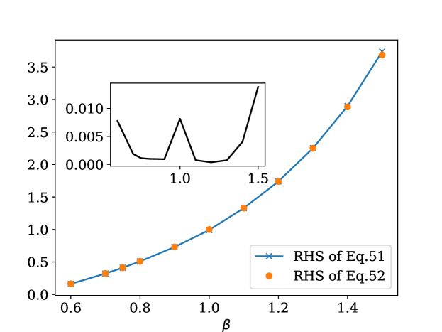
All the coefficients in the above expressions are explicit and we have evaluated numerically the right hand sides of Eqs. (5152) for values of β(0.5,1.5)𝛽0.51.5\beta\in(0.5,1.5). In Fig. (7), we plot these quantities and find that they are very close to each other, hence verifying the Green-Kubo formula Eq. (41) for general β𝛽\beta. The differences arise from numerical error due to truncation of series and also use of a finite number of basis functions. For β=1𝛽1\beta=1, this leads to diffusive results for which the double summation can be computed explicitly. Conversely, on the basis of the validity of the Green-Kubo formula we are then led to conjecture a mathematical identity between the right hand sides of Eqs. (5152). For β<1/2𝛽12\beta<1/2, one has a non-convergent series summation in Eq. (52), which leads to a breakdown of the identity in this form. This corresponds to defining zeta function for power less than 111, and possibly analytic continuation could extend the definition to other values of β𝛽\beta. We believe that the relation holds true at least in the open interval β(1/2,3/2)𝛽1232\beta\in(1/2,3/2). However, proving it remains an open problem.
Refer to caption
Figure 7: The numerically evaluated expressions in Eq. (51) and Eq. (52) are plotted as a function of general fractional power β𝛽\beta. The two quantities match numerically to a very good precision. The relative error between the two is plotted in the inset.

4.4 Long range correlations in NESS

For a noneqlibrium current carrying steady state, it is expected that fluctuations across the system will develop non-zero long-range correlations. These long-range correlations is a distinguishing feature of non-equilibrium systems with conservative dynamics [27]. In some diffusive lattice gas as well as some Hamiltonian systems, these long-range correlations have been studied [28, 29, 30, 31, 21]. The energy correlation in the velocity flip model (HCMF) in NESS is defined as CNESS(x,y)=e(x,t)e(y,t)subscript𝐶𝑁𝐸𝑆𝑆𝑥𝑦delimited-⟨⟩𝑒𝑥𝑡𝑒𝑦𝑡C_{NESS}(x,y)=\langle e(x,t)e(y,t)\rangle, where the average is taken in NESS (as t𝑡t\to\infty). It was shown that CNESS(x,y)=δT2Δ1(x,y)subscript𝐶𝑁𝐸𝑆𝑆𝑥𝑦𝛿superscript𝑇2superscriptΔ1𝑥𝑦C_{NESS}(x,y)=\delta T^{2}\Delta^{-1}(x,y), where ΔΔ\Delta is the Laplacian operator with Dirichlet boundary conditions. From the definition of fluctuating fractional equation in equilibrium, it is tempting to extend the definition of fluctuating fractional equation to non-equilibrium case, where the temperature is space-dependent:

t|etsubscript𝑡ketsubscript𝑒𝑡\displaystyle\partial_{t}|\;e_{t}\;\rangle =𝕃κ¯|et+2κ¯(BTNESS|ηt),absentsubscript𝕃¯𝜅ketsubscript𝑒𝑡2¯𝜅𝐵subscript𝑇𝑁𝐸𝑆𝑆ketsubscript𝜂𝑡\displaystyle=-\mathbb{L}_{\bar{\kappa}}|\;e_{t}\;\rangle+\sqrt{2\bar{\kappa}}\nabla(BT_{NESS}|\;\eta_{t}\;\rangle), (56)

We note that there is an ambiguity regarding the relative position of the operator B𝐵B and TNESSsubscript𝑇𝑁𝐸𝑆𝑆T_{NESS}, and also with the definition for operator B𝐵B and Bsuperscript𝐵B^{\dagger} separately. If we anyway proceed with a naive replacement of T𝑇T by TNESS(x)subscript𝑇𝑁𝐸𝑆𝑆𝑥T_{NESS}(x) in Eq. (31), to get (56), we can perform the computation of CNESS(x,y)subscript𝐶𝑁𝐸𝑆𝑆𝑥𝑦C_{NESS}(x,y) and find that this does not agree with the results from direct simulations. However, in analogy to the HCMF model, we conjecture that the NESS energy correlations CNESS(x,y)subscript𝐶𝑁𝐸𝑆𝑆𝑥𝑦C_{NESS}(x,y) are given (upto a constant factor ν𝜈\nu) by the inverse of the fractional Laplacian (in Dirichlet basis):

δT2(x,y)=δT2ν𝕃1=δT2νn1ψn(x)ψn(y)μn,𝛿superscript𝑇2𝑥𝑦𝛿superscript𝑇2𝜈superscript𝕃1𝛿superscript𝑇2𝜈subscript𝑛1subscript𝜓𝑛𝑥subscript𝜓𝑛𝑦subscript𝜇𝑛\displaystyle\delta T^{2}\mathbb{C}(x,y)=\frac{\delta T^{2}}{\nu}\mathbb{L}^{-1}=\frac{\delta T^{2}}{\nu}\sum_{n\geq 1}\frac{\psi_{n}(x)\psi_{n}(y)}{\mu_{n}}, (57)

where we have defined δT2(x,y)=CNESS(x,y)TNESS(x)2δ(xy)𝛿superscript𝑇2𝑥𝑦subscript𝐶𝑁𝐸𝑆𝑆𝑥𝑦subscript𝑇𝑁𝐸𝑆𝑆superscript𝑥2𝛿𝑥𝑦\delta T^{2}\mathbb{C}(x,y)=C_{NESS}(x,y)-T_{NESS}(x)^{2}\delta(x-y), with the local same-site correlation TNESS(x)2δ(xy)subscript𝑇𝑁𝐸𝑆𝑆superscript𝑥2𝛿𝑥𝑦T_{NESS}(x)^{2}\delta(x-y) subtracted from correlations.

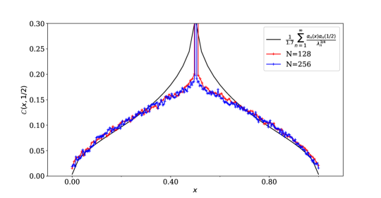
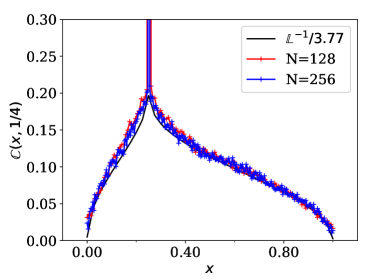
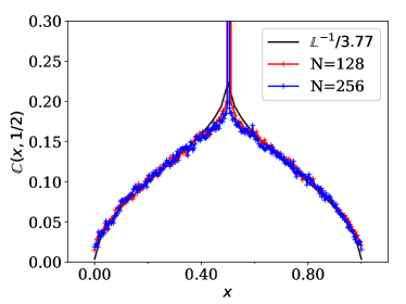
Numerical verification of Eq. (8): We simulate the microscopic system in non-equilibrium with two Langevian heat baths kept at different temperature. After the system is in the steady state, we compute (x,y)=Ne(i/N)e(j/N)𝑥𝑦𝑁delimited-⟨⟩𝑒𝑖𝑁𝑒𝑗𝑁\mathbb{C}(x,y)=N\langle e(i/N)e(j/N)\rangle where e(i/N)=E(i/N)E(i/N)𝑒𝑖𝑁𝐸𝑖𝑁delimited-⟨⟩𝐸𝑖𝑁e(i/N)=E(i/N)-\langle E(i/N)\rangle. In Fig. (8) we compare our conjectured form from Eq.  (57) with the results from microscopic simulations. We see that with the constant ν3.77𝜈3.77\nu\approx 3.77, the two numerical curves (for y=1/4𝑦14y=1/4 and y=1/2𝑦12y=1/2) match well with the inverse of fractional Laplacian. The constant ν𝜈\nu is related to the total energy fluctuations in the system at NESS as

01𝑑x01𝑑yδT2ν𝕃1(x,y)+01𝑑xTNESS2(x)=01𝑑x01𝑑yCNESS(x,y)=ΔEtot2NESS.superscriptsubscript01differential-d𝑥superscriptsubscript01differential-d𝑦𝛿superscript𝑇2𝜈superscript𝕃1𝑥𝑦superscriptsubscript01differential-d𝑥subscriptsuperscript𝑇2𝑁𝐸𝑆𝑆𝑥superscriptsubscript01differential-d𝑥superscriptsubscript01differential-d𝑦subscript𝐶𝑁𝐸𝑆𝑆𝑥𝑦subscriptdelimited-⟨⟩Δsuperscriptsubscript𝐸𝑡𝑜𝑡2𝑁𝐸𝑆𝑆\displaystyle\int_{0}^{1}dx\int_{0}^{1}dy\frac{\delta T^{2}}{\nu}\mathbb{L}^{-1}(x,y)+\int_{0}^{1}dxT^{2}_{NESS}(x)=\int_{0}^{1}dx\int_{0}^{1}dy~{}C_{NESS}(x,y)=\big{\langle}\Delta E_{tot}^{2}\big{\rangle}_{NESS}.

By evaluating the integrals on the LHS and finding the RHS from numerical simulations in the NESS, we can use the above equation to independently evaluate ν𝜈\nu. We find that the fluctuations ΔEtot2NESSsubscriptdelimited-⟨⟩Δsuperscriptsubscript𝐸𝑡𝑜𝑡2𝑁𝐸𝑆𝑆\big{\langle}\Delta E_{tot}^{2}\big{\rangle}_{NESS}, obtained from simulations in NESS, converges very slowly and with the final accessed simulation time (2×1092superscript1092\times 10^{9} time with 108superscript10810^{8} samples) we estimate 3.51ν4.23.51𝜈4.23.51\leq\nu\leq 4.2. The value ν3.77𝜈3.77\nu\approx 3.77, obtained by fitting the long range correlations data from simulation, is well within the limits of the above estimate. We have tested (see F) that the constant ν𝜈\nu does not change substantially with δT𝛿𝑇\delta T and T¯¯𝑇\bar{T}, within the numerical accuracy and finite size effects. We note in F, that if we did the same computation with sin(nπx)𝑛𝜋𝑥\sin(n\pi x) basis, then the results would differ significantly. We close this section by making a comment that proving our conjecture on the equality between the long-range correlations and the inverse fractional operator is an open question.
Refer to caption
Refer to caption
Figure 8: Non-equilibrium energy correlation function (x,y)𝑥𝑦\mathbb{C}(x,y) in steady state of Harmonic chain momentum exchange model for y=1/4𝑦14y=1/4 (left figure) and y=1/2𝑦12y=1/2 (right figure). The system size considered here are for N=128,256𝑁128256N=128,256 with TL=2,TR=1formulae-sequencesubscript𝑇𝐿2subscript𝑇𝑅1T_{L}=2,T_{R}=1 . The inverse of the fractional Laplacian (summed up to 600 basis states) and with an arbitrary constant factor (ν=3.77𝜈3.77\nu=3.77), is plotted (black solid) along with the simulation results.

5 Conclusions

We have shown that in a particular analytically tractable model of heat conduction in one dimension, the macroscopic evolution of energy in an open system is governed by the fractional diffusion equation. This gives us a definition of the fractional operator in a finite domain and also gives a meaning to the fractional operator in terms of linear PDE’s (similar to the harmonic extension of a fractional operator). We describe an efficient procedure to numerically construct the eigenspectrum of this operator. In terms of this operator, we compute the steady state and time evolution of temperature field, which we compare with microscopic simulations of the system. We defined the fluctuating fractional equation and used it to verify the Green-Kubo relation in the system. We also generalize the Green-Kubo for general fractional power which leads to some general mathematical identity involving zeta functions. This identity is verified numerically. We also conjecture that the long-range correlations are given by the inverse of a fractional operator. Proving this conjecture in Eq. (57), as well as finding the correct equation to replace Eq. (56) are open problems. The other interesting question would be to consider the use of the fractional operator in studying the dynamics of other Hamiltonian systems such as the FPUT model and also the HCME model with other boundary conditions. Another very interesting aspect is to study the usefulness of the eigensystem of the fractional operators in studying other applications where the underlying dynamics can be modelled as Levy flights or Levy walks.

6 Acknowledgments

The authors are very grateful to G. Basile, T. Komorowski and S. Olla to send them their unpublished notes [19] on which a part of this work is based. Aritra Kundu would like to thank the hospitality of Nice Sophia-Antipolis University Laboratoire Dieudonné and Institut Henri Poincaré - Centre Emile Borel during the trimester “Stochastic Dynamics Out of Equilibrium” where part of the work was done. This work benefited from the support of the project EDNHS ANR-14-CE25-0011 of the French National Research Agency (ANR), and also in part by the International Centre for Theoretical Sciences (ICTS) during a visit for participating in the program Non-equilibrium statistical physics (Code: ICTS/Prog-NESP/2015/10). Cédric Bernardin thanks the French National Research Agency (ANR) for its support through the grant ANR-15-CE40-0020-01 (LSD) and the European Research Council (ERC) under the European Union’s Horizon 2020 research and innovative programme (grant agreement No 715734). Anupam Kundu (AK) would like to acknowledge the support from DST grant under project No. ECR/2017/000634. AK, AD and CB would like to acknowledge the support from the project 5604-2 of the Indo-French Centre for the Promotion of Advanced Research (IFCPAR). KS was supported by JSPS Grants-in-Aid for Scientic Research (JP16H02211 and JP17K05587).

7 References

References

  • [1] Lepri S, 2016 Thermal Transport in Low Dimensions: From Statistical Physics to Nanoscale Heat Transfer 1st ed vol 921 (Springer International Publishing Switzerland 2016) ISBN 978-3-319-29259-5
  • [2] Lepri S, Livi R and Politi A, Thermal conduction in classical low-dimensional lattices, 2003 Physics Reports, 377(1) 1–80
  • [3] Dhar A, Heat transport in low-dimensional systems, 2008 Advances in Physics, 57(5) 457–537
  • [4] Van Beijeren H, Exact results for anomalous transport in one-dimensional hamiltonian systems, 2012 Physical Review Letters, 108(18)
  • [5] Spohn H, Nonlinear Fluctuating Hydrodynamics for Anharmonic Chains, 2014 Journal of Statistical Physics, 154(5) 1191–1227
  • [6] Mendl C B and Spohn H, Dynamic correlators of Fermi-Pasta-Ulam chains and nonlinear fluctuating hydrodynamics, 2013 Physical Review Letters, 111(23)
  • [7] Popkov V, Schadschneider A, Schmidt J and Schütz G M, Exact scaling solution of the mode coupling equations for non-linear fluctuating hydrodynamics in one dimension, 2016 Journal of Statistical Mechanics: Theory and Experiment, 2016(9)
  • [8] Narayan O and Ramaswamy S, Anomalous Heat Conduction in One-Dimensional Momentum-Conserving Systems, 2002 Physical Review Letters, 89(20)
  • [9] Das S G, Dhar A and Narayan O, Heat Conduction in the α𝛼\alpha-β𝛽\beta Fermi-Pasta-Ulam Chain, 2014 Journal of Statistical Physics, 154(1-2) 204–213
  • [10] Bernardin C and Stoltz G, Anomalous diffusion for a class of systems with two conserved quantities, 2012 Nonlinearity, 25(4) 1099–1133
  • [11] Lepri S, Mejía-Monasterio C and Politi A, A stochastic model of anomalous heat transport: Analytical solution of the steady state, 2009 Journal of Physics A: Mathematical and Theoretical, 42(2)
  • [12] Lepri S, Mejía-Monasterio C and Politi A, Nonequilibrium dynamics of a stochastic model of anomalous heat transport, 2010 Journal of Physics A: Mathematical and Theoretical, 43(6)
  • [13] Delfini L, Lepri S, Livi R, Mejía-Monasterio C and Politi A, Nonequilibrium dynamics of a stochastic model of anomalous heat transport: Numerical analysis, 2010 Journal of Physics A: Mathematical and Theoretical, 43(14)
  • [14] Jara M, Komorowski T and Olla S, Superdiffusion of Energy in a Chain of Harmonic Oscillators with Noise, 2015 Communications in Mathematical Physics, 339(2) 407–453
  • [15] Bernardin C, Gonçalves P and Jara M, 3/4-Fractional Superdiffusion in a System of Harmonic Oscillators Perturbed by a Conservative Noise, 2016 Archive for Rational Mechanics and Analysis, 220(2) 505–542
  • [16] Basile G, Bernardin C and Olla S, Momentum conserving model with anomalous thermal conductivity in low dimensional systems, 2006 Physical Review Letters, 96(20) 1–4
  • [17] Viswanathan G M, Afanasyev V, Buldyrev S V, Havlin S, Da Luz M G, Raposo E P and Stanley H E, Levy flights in random searches, 2000 Physica A: Statistical Mechanics and its Applications, 282(1) 1–12
  • [18] Zoia A, Rosso A and Kardar M, Fractional Laplacian in bounded domains, 2007 Physical Review E - Statistical, Nonlinear, and Soft Matter Physics, 76(2)
  • [19] Basile G, Komorowski T and Olla S, , 2015 Private Communication,
  • [20] Cividini J, Kundu A, Miron A and Mukamel D, Temperature profile and boundary conditions in an anomalous heat transport model, 2017 Journal of Statistical Mechanics: Theory and Experiment, 013203(1)
  • [21] Bernardin C, Kannan V, Lebowitz J L and Lukkarinen J, Harmonic Systems with Bulk Noises, 2012 Journal of Statistical Physics, 146(4) 800–831
  • [22] Spohn H, 2012 Large scale dynamics of interacting particles (Springer Science & Business Media)
  • [23] Buldyrev S V, Gitterman M, Havlin S, Kazakov A Y, Da Luz M G, Raposo E P, Stanley H E and Viswanathan G M, Properties of Lévy flights on an interval with absorbing boundaries, 2001 Physica A: Statistical Mechanics and its Applications, 302(1-4) 148–161
  • [24] Buldyrev S V, Havlin S, Kazakov A Y, da Luz M G, Raposo E P, Stanley H E and Viswanathan G M, Average time spent by Lévy flights and walks on an interval with absorbing boundaries, 2001 Physical Review E - Statistical Physics, Plasmas, Fluids, and Related Interdisciplinary Topics, 64(4) 11
  • [25] Chen W and Holm S, Fractional Laplacian time-space models for linear and nonlinear lossy media exhibiting arbitrary frequency power-law dependency, 2004 The Journal of the Acoustical Society of America, 115(4) 1424–1430
  • [26] Kundu A, Dhar A and Narayan O, The green-kubo formula for heat conduction in open systems, 2009 Journal of Statistical Mechanics: Theory and Experiment, 03(03) L03001
  • [27] Garrido P L, Lebowitz J L, Maes C and Spohn H, Long-range correlations for conservative dynamics, 1990 Physical Review A, 42(4) 1954
  • [28] Spohn H, Long range correlations for stochastic lattice gases in a non-equilibrium steady state, 1983 Journal of Physics A: General Physics, 16(18) 4275–4291
  • [29] Bodineau T, Derrida B, Lecomte V and Van Wijland F, Long range correlations and phase transitions in non-equilibrium diffusive systems, 2008 Journal of Statistical Physics, 133(6) 1013–1031
  • [30] Bertini L, De Sole A, Gabrielli D, Jona-Lasinio G and Landim C, On the long range correlations of thermodynamic systems out of equilibrium, 2007 arXiv preprint arXiv:0705.2996., 1–4
  • [31] Derrida B, Non-equilibrium steady states: fluctuations and large deviations of the density and of the current, 2007 Journal of Statistical Mechanics: Theory and Experiment, 2007(07) P07023

Appendix A Connection coefficients between sine and cosine

We can expand sin\sin in the complete basis of cos\cos as, αn(y)=l𝒯nlϕl(y)subscript𝛼𝑛𝑦subscript𝑙subscript𝒯𝑛𝑙subscriptitalic-ϕ𝑙𝑦\alpha_{n}(y)=\sum_{l}\mathcal{T}_{nl}\phi_{l}(y), with explicit coefficients 𝒯nl=01𝑑yαn(y)ϕl(y)subscript𝒯𝑛𝑙superscriptsubscript01differential-d𝑦subscript𝛼𝑛𝑦subscriptitalic-ϕ𝑙𝑦\mathcal{T}_{nl}=\int_{0}^{1}dy\alpha_{n}(y)\phi_{l}(y). The coefficients are given as,

𝒯nl=subscript𝒯𝑛𝑙absent\displaystyle\mathcal{T}_{nl}= {0if l=0, n is even,22πnif l=0, n is odd,2π[δ(n+l),oddn+l+δ(nl),oddnl],ifl>0.cases0if l=0, n is even,otherwise22𝜋𝑛if l=0, n is odd,otherwise2𝜋delimited-[]subscript𝛿𝑛𝑙odd𝑛𝑙subscript𝛿𝑛𝑙odd𝑛𝑙if𝑙0otherwise\displaystyle\begin{cases}0~{}\text{if l=0, n is even,}\\ \frac{2\sqrt{2}}{\pi n}~{}\text{if l=0, n is odd,}\\ \frac{2}{\pi}\left[\frac{\delta_{(n+l),\text{odd}}}{n+l}+\frac{\delta_{(n-l),\text{odd}}}{n-l}\right],~{}\text{if}~{}l>0.\end{cases} (58)

Appendix B Derivation of matrix equations of Fractional operator

Here we enumerate the steps involved in going from the set of PDE’s to the matrix representation of 𝕃𝕃\mathbb{L} as stated in the main text. The correlation and temperature fields are expanded as, C(x,y,τ)Css(x,y)=n=1C^n(x,τ)αn(y)𝐶𝑥𝑦𝜏subscript𝐶𝑠𝑠𝑥𝑦superscriptsubscript𝑛1subscript^𝐶𝑛𝑥𝜏subscript𝛼𝑛𝑦C(x,y,\tau)-C_{ss}(x,y)=\sum_{n=1}^{\infty}\hat{C}_{n}(x,\tau)\alpha_{n}(y) and T(y,τ)Tss(y)=f(y,τ)=n=1f^n(τ)αn(y).𝑇𝑦𝜏subscript𝑇𝑠𝑠𝑦𝑓𝑦𝜏superscriptsubscript𝑛1subscript^𝑓𝑛𝜏subscript𝛼𝑛𝑦T(y,\tau)-T_{ss}(y)=f(y,\tau)=\sum_{n=1}^{\infty}\hat{f}_{n}(\tau)\alpha_{n}(y). Following [12], the first of the equations in (3) implies x4C^n(x)=4δn4C^n(x)subscriptsuperscript4𝑥subscript^𝐶𝑛𝑥4superscriptsubscript𝛿𝑛4subscript^𝐶𝑛𝑥\partial^{4}_{x}\hat{C}_{n}(x)=-4\delta_{n}^{4}\hat{C}_{n}(x), where δn=nπω/(2γ)subscript𝛿𝑛𝑛𝜋𝜔2𝛾\delta_{n}=\sqrt{n\pi\omega/(2\gamma)}. Solving these equations with the appropriate boundary conditions one eventually gets,

C^n(x,τ)=A^n(τ)eδnx[sin(δnx)cos(δnx)].subscript^𝐶𝑛𝑥𝜏subscript^𝐴𝑛𝜏superscript𝑒subscript𝛿𝑛𝑥delimited-[]subscript𝛿𝑛𝑥subscript𝛿𝑛𝑥\displaystyle\hat{C}_{n}(x,\tau)=\hat{A}_{n}(\tau)e^{-\delta_{n}x}~{}[\sin(\delta_{n}x)-\cos(\delta_{n}x)]~{}. (59)

using the PDE’s one gets

A^n(τ)subscript^𝐴𝑛𝜏\displaystyle\hat{A}_{n}(\tau) =14γδnk=1𝒯knλkfkabsent14𝛾subscript𝛿𝑛subscript𝑘1superscriptsubscript𝒯𝑘𝑛subscript𝜆𝑘subscript𝑓𝑘\displaystyle=-\frac{1}{4\gamma\delta_{n}}\sum_{k=1}\mathcal{T}_{kn}^{\dagger}\sqrt{\lambda_{k}}f_{k}
f^˙msubscript˙^𝑓𝑚\displaystyle\dot{\hat{f}}_{m} =ω2n=1𝒯mnλnA^n(τ)absentsuperscript𝜔2subscript𝑛1subscript𝒯𝑚𝑛subscript𝜆𝑛subscript^𝐴𝑛𝜏\displaystyle=\omega^{2}\sum_{n=1}\mathcal{T}_{mn}\sqrt{\lambda_{n}}\hat{A}_{n}(\tau)
=\displaystyle= ω24γn,k=1𝒯mnλn1δn𝒯knλkfksuperscript𝜔24𝛾subscript𝑛𝑘1subscript𝒯𝑚𝑛subscript𝜆𝑛1subscript𝛿𝑛superscriptsubscript𝒯𝑘𝑛subscript𝜆𝑘subscript𝑓𝑘\displaystyle-\frac{\omega^{2}}{4\gamma}\sum_{n,k=1}\mathcal{T}_{mn}\sqrt{\lambda_{n}}\frac{1}{\delta_{n}}\mathcal{T}_{kn}^{\dagger}\sqrt{\lambda_{k}}f_{k}
=\displaystyle= ω24γn,k=1𝒯mnλnδn𝒯nkfksuperscript𝜔24𝛾subscript𝑛𝑘1subscript𝒯𝑚𝑛subscript𝜆𝑛subscript𝛿𝑛superscriptsubscript𝒯𝑛𝑘subscript𝑓𝑘\displaystyle-\frac{\omega^{2}}{4\gamma}\sum_{n,k=1}\mathcal{T}_{mn}\frac{\lambda_{n}}{\delta_{n}}\mathcal{T}_{nk}^{\dagger}f_{k}
=\displaystyle= κ¯[𝒯Λ3/4𝒯]mkfk¯𝜅subscriptdelimited-[]𝒯superscriptΛ34superscript𝒯𝑚𝑘subscript𝑓𝑘\displaystyle-\bar{\kappa}\left[\mathcal{T}\Lambda^{3/4}\mathcal{T}^{\dagger}\right]_{mk}f_{k} (60)

where we used the property of transformation element, 𝒯knλk=𝒯knλnsuperscriptsubscript𝒯𝑘𝑛subscript𝜆𝑘subscript𝒯𝑘𝑛subscript𝜆𝑛\mathcal{T}_{kn}^{\dagger}\sqrt{\lambda_{k}}=\mathcal{T}_{kn}\sqrt{\lambda_{n}}. with 𝒯nl=αn|ϕl=01𝑑yαn(y)ϕl(y)subscript𝒯𝑛𝑙inner-productsubscript𝛼𝑛subscriptitalic-ϕ𝑙superscriptsubscript01differential-d𝑦subscript𝛼𝑛𝑦subscriptitalic-ϕ𝑙𝑦\mathcal{T}_{nl}=\langle\alpha_{n}|\phi_{l}\rangle=\int_{0}^{1}dy\alpha_{n}(y)\phi_{l}(y) and the constant κ¯¯𝜅\bar{\kappa}.

Appendix C Formal identities of cos and sin series

Consider the two Fourier cosine series on [0,1]01[0,1],

q=𝑞absent\displaystyle q= 12+modd22π2m22cos(πmq),12subscript𝑚𝑜𝑑𝑑22superscript𝜋2superscript𝑚22𝜋𝑚𝑞\displaystyle~{}\frac{1}{2}+\sum_{m\;odd}\frac{-2\sqrt{2}}{\pi^{2}m^{2}}\sqrt{2}\cos(\pi mq),
q2q=superscript𝑞2𝑞absent\displaystyle q^{2}-q= 16+meven22π2m22cos(πmq),16subscript𝑚𝑒𝑣𝑒𝑛22superscript𝜋2superscript𝑚22𝜋𝑚𝑞\displaystyle-\frac{1}{6}+\sum_{m\in even}\frac{2\sqrt{2}}{\pi^{2}m^{2}}\sqrt{2}\cos(\pi mq), (61)
q2q=superscript𝑞2𝑞absent\displaystyle q^{2}-q= modd42(nπ)32sin(πmq).subscript𝑚𝑜𝑑𝑑42superscript𝑛𝜋32𝜋𝑚𝑞\displaystyle\sum_{m\in odd}-\frac{4\sqrt{2}}{(n\pi)^{3}}\sqrt{2}\sin(\pi mq).

Formally differentiating these two equations with respect to q𝑞q on both sides we get two formal identities (which needs to be interpreted as distributional sense):

moddcos(πmq)=subscript𝑚𝑜𝑑𝑑𝑐𝑜𝑠𝜋𝑚𝑞absent\displaystyle\sum_{m\;odd}cos(\pi mq)= 00\displaystyle~{}0 (62)
meven,m>12cos(πmq)=subscript𝑚𝑒𝑣𝑒𝑛𝑚12𝑐𝑜𝑠𝜋𝑚𝑞absent\displaystyle\sum_{\begin{subarray}{c}m\;even,\\ m>1\end{subarray}}\sqrt{2}cos(\pi mq)= 12,12\displaystyle-\frac{1}{\sqrt{2}}, (63)
modd2sin(mπq)λn=subscript𝑚𝑜𝑑𝑑2𝑚𝜋𝑞subscript𝜆𝑛absent\displaystyle\sum_{m\;odd}\frac{\sqrt{2}\sin(m\pi q)}{\sqrt{\lambda_{n}}}= 122.122\displaystyle\frac{1}{2\sqrt{2}}. (64)

Appendix D Alternate series representation of BB𝐵superscript𝐵BB^{\dagger} and connection with Eq. (36)

As mentioned in the main text the kernel operator BB𝐵superscript𝐵BB^{\dagger} has appeared earlier in the context of heat conduction through HCME model [20]. Using non-linear hydrodynamics theory in [20], the non-local linear response relation has been established for general boundary conditions characterized by a reflection coefficient R=(λωλ+ω)2𝑅superscript𝜆𝜔𝜆𝜔2R=\left(\frac{\lambda-\omega}{\lambda+\omega}\right)^{2} which vary from 00 to 111. For given R𝑅R, the expression for the kernel is given as [20]

BB(x,x)=12πn=[R|2n||2n+xx|R|2n+1||2n+x+x|].𝐵superscript𝐵𝑥superscript𝑥12𝜋superscriptsubscript𝑛delimited-[]superscript𝑅2𝑛2𝑛𝑥superscript𝑥superscript𝑅2𝑛12𝑛𝑥superscript𝑥\displaystyle BB^{\dagger}(x,x^{\prime})=\frac{1}{\sqrt{2\pi}}\sum_{n=-\infty}^{\infty}\left[\frac{R^{|2n|}}{\sqrt{|2n+x-x^{\prime}|}}-\frac{R^{|2n+1|}}{\sqrt{|2n+x+x^{\prime}|}}\right]. (65)

The value R=0𝑅0R=0 corresponds to the resonance condition ω=λ𝜔𝜆\omega=\lambda for free boundary condition i.e. q0=q1subscript𝑞0subscript𝑞1q_{0}=q_{1} and qN=qN+1subscript𝑞𝑁subscript𝑞𝑁1q_{N}=q_{N+1}. On the other hand, R=1𝑅1R=1 corresponds to fixed boundary condition. For R=1𝑅1R=1, one can explicitly check with the above representation that

01𝑑xBB(x,x)αm(x)=1λn1/4αm(x),superscriptsubscript01differential-dsuperscript𝑥𝐵superscript𝐵𝑥superscript𝑥subscript𝛼𝑚superscript𝑥1superscriptsubscript𝜆𝑛14subscript𝛼𝑚𝑥\displaystyle\int_{0}^{1}dx^{\prime}~{}BB^{\dagger}(x,x^{\prime})\alpha_{m}(x^{\prime})=\frac{1}{\lambda_{n}^{1/4}}\alpha_{m}(x), (66)

which is same as Eq. (36). The proof is as follows. The LHS of Eq. (66) can be written as,

L.H.S=1π01dy[1|xy|\displaystyle L.H.S=\frac{1}{\sqrt{\pi}}\int_{0}^{1}dy\Bigg{[}\frac{1}{\sqrt{|x-y|}} +n=112n+xy+12nx+ysuperscriptsubscript𝑛112𝑛𝑥𝑦12𝑛𝑥𝑦\displaystyle+\sum_{n=1}^{\infty}\frac{1}{\sqrt{2n+x-y}}+\frac{1}{\sqrt{2n-x+y}}
12n2+x+y12nxy]sin(mπy)\displaystyle-\frac{1}{\sqrt{2n-2+x+y}}-\frac{1}{\sqrt{2n-x-y}}\Bigg{]}\sin(m\pi y) (67)

Using change of variables and separating the part in absolute value we have,

L.H.S=1π[0xdz\displaystyle L.H.S=\frac{1}{\sqrt{\pi}}\Bigg{[}\int_{0}^{x}dz sin(mπ(xz))z+01x𝑑zsin(mπ(x+z))z𝑚𝜋𝑥𝑧𝑧superscriptsubscript01𝑥differential-d𝑧𝑚𝜋𝑥𝑧𝑧\displaystyle\frac{\sin(m\pi(x-z))}{\sqrt{z}}+\int_{0}^{1-x}dz\frac{\sin(m\pi(x+z))}{\sqrt{z}}
+\displaystyle+ n=1(2n1+x2n+xdzsin(mπ(2n+xz))z+2nx2n+1xdzsin(mπ(z2n+x))z\displaystyle\sum_{n=1}^{\infty}\Bigg{(}\int_{2n-1+x}^{2n+x}dz\frac{\sin(m\pi(2n+x-z))}{\sqrt{z}}+\int_{2n-x}^{2n+1-x}dz\frac{\sin(m\pi(z-2n+x))}{\sqrt{z}}
\displaystyle- 2n2+x2n1+xdzsin(mπ(z2n+2x))z2n1x2nxdzsin(mπ(2nxz))z)]\displaystyle\int^{2n-1+x}_{2n-2+x}dz\frac{\sin(m\pi(z-2n+2-x))}{\sqrt{z}}-\int^{2n-x}_{2n-1-x}dz\frac{\sin(m\pi(2n-x-z))}{\sqrt{z}}\Bigg{)}\Bigg{]}

Upon using trigonometric identities this can be reduced to,

L.H.S.=1π[(0xdz+n=1(2n2+x2n1+xdz+2n1+x2n+x))sin(mπ(xz))z\displaystyle L.H.S.=\frac{1}{\sqrt{\pi}}\Bigg{[}\Bigg{(}\int_{0}^{x}dz+\sum_{n=1}^{\infty}\Big{(}\int^{2n-1+x}_{2n-2+x}dz+\int_{2n-1+x}^{2n+x}\Big{)}\Bigg{)}\frac{\sin(m\pi(x-z))}{\sqrt{z}}
+(01xdz+n=1(2n1x2nxdz+2nx2n+1x))sin(mπ(x+z))z]\displaystyle+\Bigg{(}\int_{0}^{1-x}dz+\sum_{n=1}^{\infty}\Big{(}\int^{2n-x}_{2n-1-x}dz+\int^{2n+1-x}_{2n-x}\Big{)}\Bigg{)}\frac{\sin(m\pi(x+z))}{\sqrt{z}}\Bigg{]} (68)

which, upon simplifying further provides the R.H.S. of Eq. (66),

1π0𝑑z[sin(mπ(xz))z+sin(mπ(x+z))z]=1mπ2sin(mπx)1𝜋superscriptsubscript0differential-d𝑧delimited-[]𝑚𝜋𝑥𝑧𝑧𝑚𝜋𝑥𝑧𝑧1𝑚𝜋2𝑚𝜋𝑥\displaystyle\frac{1}{\sqrt{\pi}}\int_{0}^{\infty}dz\Bigg{[}\frac{\sin(m\pi(x-z))}{\sqrt{z}}+\frac{\sin(m\pi(x+z))}{\sqrt{z}}\Bigg{]}=\frac{1}{\sqrt{m\pi}}\sqrt{2}\sin(m\pi x) (69)

Appendix E Explicit expressions of some equations mentioned in maintext

The total fractional equation (31) can be written explicitly as,

te(x,t)subscript𝑡𝑒𝑥𝑡\displaystyle\partial_{t}e(x,t) =x𝑑x[𝔸(x,t)e(x,t)B(x,t)Tη(x,t)]absentsubscript𝑥differential-dsuperscript𝑥delimited-[]𝔸superscript𝑥𝑡𝑒superscript𝑥𝑡𝐵superscript𝑥𝑡𝑇𝜂superscript𝑥𝑡\displaystyle=\nabla_{x}\int dx^{\prime}\left[{\mathbb{A}}(x^{\prime},t)e(x^{\prime},t)-B(x^{\prime},t)T\eta(x^{\prime},t)\right] (70)

The equation for the two time equilibrium spatio-temporal correlation (Eq.  (39))can be written as,

Ceq(x,t,y,t)=subscript𝐶eq𝑥𝑡𝑦superscript𝑡absent\displaystyle C_{\rm eq}(x,t,y,t^{\prime})= 2κ¯t𝑑st𝑑s𝑑x𝑑yxGtsxx(BTη)(x,s)(BTη)(y,s)yGtsyy2¯𝜅superscriptsubscript𝑡differential-d𝑠superscriptsubscriptsuperscript𝑡differential-dsuperscript𝑠differential-dsuperscript𝑥differential-dsuperscript𝑦subscriptsuperscript𝑥superscriptsubscript𝐺𝑡𝑠𝑥superscript𝑥delimited-⟨⟩𝐵𝑇𝜂superscript𝑥𝑠𝐵𝑇𝜂superscript𝑦superscript𝑠subscriptsuperscript𝑦superscriptsubscript𝐺superscript𝑡superscript𝑠𝑦superscript𝑦\displaystyle 2\bar{\kappa}\int_{-\infty}^{t}ds~{}\int_{-\infty}^{t^{\prime}}ds^{\prime}\int dx^{\prime}\int dy^{\prime}\nabla_{x^{\prime}}G_{t-s}^{xx^{\prime}}\big{\langle}{(BT\eta)}(x^{\prime},s)(BT\eta)(y^{\prime},s^{\prime})\big{\rangle}{\nabla_{y^{\prime}}G_{t^{\prime}-s^{\prime}}^{yy^{\prime}}} (71)

The spatio-temporal current correlations in Eq.  (43) can be explicitly written as,

j(x,t)j(y,t)=𝑑x𝑑yκ¯2𝔸(x,x)𝔸(y,y)e(x,t)e(y,t)delimited-⟨⟩𝑗𝑥𝑡𝑗𝑦superscript𝑡differential-dsuperscript𝑥differential-dsuperscript𝑦superscript¯𝜅2𝔸𝑥superscript𝑥𝔸𝑦superscript𝑦delimited-⟨⟩𝑒superscript𝑥𝑡𝑒superscript𝑦superscript𝑡\displaystyle\big{\langle}j(x,t)j(y,t^{\prime})\big{\rangle}=\int dx^{\prime}\int dy^{\prime}\bar{\kappa}^{2}\mathbb{A}(x,x^{\prime})\mathbb{A}(y,y^{\prime})\big{\langle}e(x^{\prime},t)e(y^{\prime},t^{\prime})\big{\rangle} (72)
+2κ¯T2B(x,x)B(y,y)η(x,t)η(y,t)2¯𝜅superscript𝑇2𝐵𝑥superscript𝑥𝐵𝑦superscript𝑦delimited-⟨⟩𝜂superscript𝑥𝑡𝜂superscript𝑦superscript𝑡\displaystyle+2\bar{\kappa}T^{2}B(x,x^{\prime})B(y,y^{\prime})\big{\langle}\eta(x^{\prime},t)\eta(y^{\prime},t^{\prime})\big{\rangle} (73)
2κ¯3/2T𝔸(x,x)B(y,y)e(x,t)η(y,t)2superscript¯𝜅32𝑇𝔸𝑥superscript𝑥𝐵𝑦superscript𝑦delimited-⟨⟩𝑒superscript𝑥𝑡𝜂superscript𝑦superscript𝑡\displaystyle-\sqrt{2}\bar{\kappa}^{3/2}T\mathbb{A}(x,x^{\prime})B(y,y^{\prime})\big{\langle}e(x^{\prime},t)\eta(y^{\prime},t^{\prime})\big{\rangle} (74)
2κ¯3/2TB(x,x)𝔸(y,y)η(x,t)e(y,t)2superscript¯𝜅32𝑇𝐵𝑥superscript𝑥𝔸𝑦superscript𝑦delimited-⟨⟩𝜂superscript𝑥𝑡𝑒superscript𝑦superscript𝑡\displaystyle-\sqrt{2}\bar{\kappa}^{3/2}TB(x,x^{\prime})\mathbb{A}(y,y^{\prime})\big{\langle}\eta(x^{\prime},t)e(y^{\prime},t^{\prime})\big{\rangle} (75)

Since it might be a bit confusing using the symbolic vector notation for the operations in the main text, here we show explicitly the expressions for individual terms and show the 2nd and 3rd terms give a similar term to 1st. Eq.  (72) gives,

κ¯2𝑑x𝑑y𝔸(x,x)𝔸(y,y)G|tt|xysuperscript¯𝜅2differential-dsuperscript𝑥differential-dsuperscript𝑦𝔸𝑥superscript𝑥𝔸𝑦superscript𝑦subscriptsuperscript𝐺superscript𝑥superscript𝑦𝑡superscript𝑡\displaystyle\bar{\kappa}^{2}\int dx^{\prime}\int dy^{\prime}\mathbb{A}(x,x^{\prime})\mathbb{A}(y,y^{\prime})G^{x^{\prime}y^{\prime}}_{|t-t^{\prime}|} =κ¯2𝑑x𝑑yBB(x,x)xBB(y,y)yG|tt|xyabsentsuperscript¯𝜅2differential-dsuperscript𝑥differential-dsuperscript𝑦𝐵superscript𝐵𝑥superscript𝑥subscriptsuperscript𝑥𝐵superscript𝐵𝑦superscript𝑦subscriptsuperscript𝑦subscriptsuperscript𝐺superscript𝑥superscript𝑦𝑡superscript𝑡\displaystyle=\bar{\kappa}^{2}\int dx^{\prime}\int dy^{\prime}BB^{\dagger}(x,x^{\prime})\partial_{x^{\prime}}BB^{\dagger}(y,y^{\prime})\partial_{y^{\prime}}G^{x^{\prime}y^{\prime}}_{|t-t^{\prime}|}
=\displaystyle= κ¯2𝑑x𝑑y𝔸(x,x)G|tt|xy𝔸(y,y)superscript¯𝜅2differential-dsuperscript𝑥differential-dsuperscript𝑦𝔸𝑥superscript𝑥subscriptsuperscript𝐺superscript𝑥superscript𝑦𝑡superscript𝑡superscript𝔸superscript𝑦𝑦\displaystyle\bar{\kappa}^{2}\int dx^{\prime}\int dy^{\prime}\mathbb{A}(x,x^{\prime})G^{x^{\prime}y^{\prime}}_{|t-t^{\prime}|}\mathbb{A}^{\dagger}(y^{\prime},y) (76)

where we used the adjoint representation for 𝔸(y,y)=𝔸(y,y)superscript𝔸𝑦superscript𝑦𝔸superscript𝑦𝑦\mathbb{A}^{\dagger}(y,y^{\prime})=\mathbb{A}(y^{\prime},y). Eq. (74) gives,

III=IIIabsent\displaystyle\textup{III}= 𝑑x𝑑y2κ¯3/2T𝔸(x,x)B(y,y)e(x,t)η(y,t)differential-dsuperscript𝑥differential-dsuperscript𝑦2superscript¯𝜅32𝑇𝔸𝑥superscript𝑥𝐵𝑦superscript𝑦delimited-⟨⟩𝑒superscript𝑥𝑡𝜂superscript𝑦superscript𝑡\displaystyle\int dx^{\prime}\int dy^{\prime}\sqrt{2}\bar{\kappa}^{3/2}T\mathbb{A}(x,x^{\prime})B(y,y^{\prime})\big{\langle}e(x^{\prime},t)\eta(y^{\prime},t^{\prime})\big{\rangle}
=\displaystyle= 2κ¯T2𝑑x𝑑y𝑑x′′𝑑y′′t𝑑sBB(x,x)xB(y,y)Gtsxx′′x′′B(x′′,y′′)η(y′′,s)η(y,t)2¯𝜅superscript𝑇2differential-dsuperscript𝑥differential-dsuperscript𝑦differential-dsuperscript𝑥′′differential-dsuperscript𝑦′′superscriptsubscript𝑡differential-d𝑠𝐵superscript𝐵𝑥superscript𝑥subscriptsuperscript𝑥𝐵𝑦superscript𝑦subscriptsuperscript𝐺superscript𝑥superscript𝑥′′𝑡𝑠subscriptsuperscript𝑥′′𝐵superscript𝑥′′superscript𝑦′′delimited-⟨⟩𝜂superscript𝑦′′𝑠𝜂superscript𝑦superscript𝑡\displaystyle-2\bar{\kappa}T^{2}\int dx^{\prime}\int dy^{\prime}\int dx^{\prime\prime}\int dy^{\prime\prime}\int_{-\infty}^{t}dsBB^{\dagger}(x,x^{\prime})\partial_{x^{\prime}}B(y,y^{\prime})G^{x^{\prime}x^{\prime\prime}}_{t-s}\partial_{x^{\prime\prime}}B(x^{\prime\prime},y^{\prime\prime})\big{\langle}\eta(y^{\prime\prime},s)\eta(y^{\prime},t^{\prime})\big{\rangle}
=\displaystyle= 2κ¯T2𝑑x𝑑y𝑑x′′BB(x,x)xB(y,y)x′′(Gttxx′′)B(x′′,y)θ(tt)2¯𝜅superscript𝑇2differential-dsuperscript𝑥differential-dsuperscript𝑦differential-dsuperscript𝑥′′𝐵superscript𝐵𝑥superscript𝑥subscriptsuperscript𝑥𝐵𝑦superscript𝑦subscriptsuperscript𝑥′′subscriptsuperscript𝐺superscript𝑥superscript𝑥′′𝑡superscript𝑡𝐵superscript𝑥′′superscript𝑦𝜃𝑡superscript𝑡\displaystyle 2\bar{\kappa}T^{2}\int dx^{\prime}\int dy^{\prime}\int dx^{\prime\prime}BB^{\dagger}(x,x^{\prime})\partial_{x^{\prime}}B(y,y^{\prime})\partial_{x^{\prime\prime}}(G^{x^{\prime}x^{\prime\prime}}_{t-t^{\prime}})B(x^{\prime\prime},y^{\prime})\theta(t-t^{\prime})
=\displaystyle= 2κ¯T2𝑑x𝑑y𝑑x′′𝔸(x,x)Gttxx′′𝔸(x′′,y)θ(tt).2¯𝜅superscript𝑇2differential-dsuperscript𝑥differential-dsuperscript𝑦differential-dsuperscript𝑥′′𝔸𝑥superscript𝑥subscriptsuperscript𝐺superscript𝑥superscript𝑥′′𝑡superscript𝑡superscript𝔸superscript𝑥′′𝑦𝜃𝑡superscript𝑡\displaystyle 2\bar{\kappa}T^{2}\int dx^{\prime}\int dy^{\prime}\int dx^{\prime\prime}\mathbb{A}(x,x^{\prime})G^{x^{\prime}x^{\prime\prime}}_{t-t^{\prime}}\mathbb{A}^{\dagger}(x^{\prime\prime},y)\theta(t-t^{\prime}). (77)

Eq. (75) gives,

IV=IVabsent\displaystyle\textup{IV}= 𝑑x𝑑y2κ¯3/2TB(x,x)𝔸(y,y)η(x,t)e(y,t)differential-dsuperscript𝑥differential-dsuperscript𝑦2superscript¯𝜅32𝑇𝐵𝑥superscript𝑥𝔸𝑦superscript𝑦delimited-⟨⟩𝜂superscript𝑥𝑡𝑒superscript𝑦superscript𝑡\displaystyle\int dx^{\prime}\int dy^{\prime}\sqrt{2}\bar{\kappa}^{3/2}TB(x,x^{\prime})\mathbb{A}(y,y^{\prime})\big{\langle}\eta(x^{\prime},t)e(y^{\prime},t^{\prime})\big{\rangle}
=\displaystyle= 2κ¯T2𝑑x𝑑y𝑑x′′𝑑y′′t𝑑sB(x,x)𝔸(y,y)Gtsyx′′x′′B(x′′,y′′)η(x,t)η(y′′,s)2¯𝜅superscript𝑇2differential-dsuperscript𝑥differential-dsuperscript𝑦differential-dsuperscript𝑥′′differential-dsuperscript𝑦′′superscriptsubscript𝑡differential-d𝑠𝐵𝑥superscript𝑥𝔸𝑦superscript𝑦subscriptsuperscript𝐺superscript𝑦superscript𝑥′′superscript𝑡𝑠subscriptsuperscript𝑥′′𝐵superscript𝑥′′superscript𝑦′′delimited-⟨⟩𝜂superscript𝑥𝑡𝜂superscript𝑦′′𝑠\displaystyle-2\bar{\kappa}T^{2}\int dx^{\prime}\int dy^{\prime}\int dx^{\prime\prime}\int dy^{\prime\prime}\int_{-\infty}^{t}dsB(x,x^{\prime})\mathbb{A}(y,y^{\prime})G^{y^{\prime}x^{\prime\prime}}_{t^{\prime}-s}\partial_{x^{\prime\prime}}B(x^{\prime\prime},y^{\prime\prime})\big{\langle}\eta(x^{\prime},t)\eta(y^{\prime\prime},s)\big{\rangle}
=\displaystyle= 2κ¯T2𝑑x𝑑y𝑑x′′B(x,x)𝔸(y,y)x′′(Gttyx′′)B(x′′,x)θ(tt)2¯𝜅superscript𝑇2differential-dsuperscript𝑥differential-dsuperscript𝑦differential-dsuperscript𝑥′′𝐵𝑥superscript𝑥𝔸𝑦superscript𝑦subscriptsuperscript𝑥′′subscriptsuperscript𝐺superscript𝑦superscript𝑥′′superscript𝑡𝑡𝐵superscript𝑥′′superscript𝑥𝜃superscript𝑡𝑡\displaystyle 2\bar{\kappa}T^{2}\int dx^{\prime}\int dy^{\prime}\int dx^{\prime\prime}B(x,x^{\prime})\mathbb{A}(y,y^{\prime})\partial_{x^{\prime\prime}}(G^{y^{\prime}x^{\prime\prime}}_{t^{\prime}-t})B(x^{\prime\prime},x^{\prime})\theta(t^{\prime}-t)
=\displaystyle= 2κ¯T2𝑑x𝑑y𝑑x′′𝔸(y,y)Gttyx′′𝔸(x′′,x)θ(tt).2¯𝜅superscript𝑇2differential-dsuperscript𝑥differential-dsuperscript𝑦differential-dsuperscript𝑥′′𝔸𝑦superscript𝑦subscriptsuperscript𝐺superscript𝑦superscript𝑥′′superscript𝑡𝑡superscript𝔸superscript𝑥′′𝑥𝜃superscript𝑡𝑡\displaystyle 2\bar{\kappa}T^{2}\int dx^{\prime}\int dy^{\prime}\int dx^{\prime\prime}\mathbb{A}(y,y^{\prime})G^{y^{\prime}x^{\prime\prime}}_{t^{\prime}-t}\mathbb{A}^{\dagger}(x^{\prime\prime},x)\theta(t^{\prime}-t). (78)

The second term is explicit in the main-text.

Appendix F Some tests on Long-range correlations

In Fig. (9) we do microscopic simulations for different temperature differences, and absolute temperatures to show, to good accuracy, the constant ν𝜈\nu does not depend on these factors. In Fig.  (10) we test the use of α𝛼\alpha(sin) basis instead of the ψ𝜓\psi basis for theoretical prediction for the nature of long-range correlations, and show it performs badly.
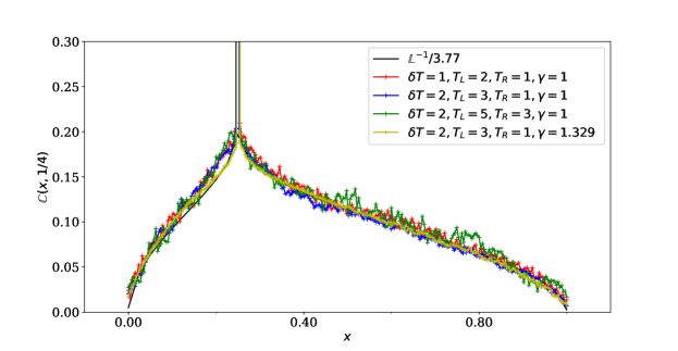
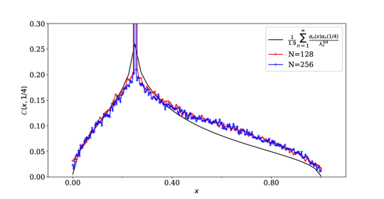
Refer to caption
Figure 9: Simulation results for N=256𝑁256N=256, with 444 different temperature and exchange rate parameters mentioned in the graph. The black curve is theoretically computed curve with ν=3.77𝜈3.77\nu=3.77, we see the results from the simulation are very close to predicted theoretical curve for the different parameters. This suggests that the parameter ν𝜈\nu is independent of absolute value of the applied boundary temperature, the temperature gradient of the system and the long range correlations do not depend on the details like the stochastic exchange rate etc. The slight differences are again, hopefully a result of finite size effect.
Refer to caption
Refer to caption
Figure 10: Here we show that instead of using ψnsubscript𝜓𝑛\psi_{n} and μnsubscript𝜇𝑛\mu_{n} if we use sin\sin and λn3/4superscriptsubscript𝜆𝑛34\lambda_{n}^{3/4} for construction of inverse of the fractional operator, there are significant difference between the simulations with the formula (x,y)=n=1αn(x)αn(y)λn3/4𝑥𝑦superscriptsubscript𝑛1subscript𝛼𝑛𝑥subscript𝛼𝑛𝑦superscriptsubscript𝜆𝑛34\mathbb{C}(x,y)=\sum_{n=1}^{\infty}\frac{\alpha_{n}(x)\alpha_{n}(y)}{\lambda_{n}^{3/4}}