Numerical solutions of Fokker-Planck equations with drift-admitting jumps

Abstract

We develop a finite difference scheme based on a grid staggered by flux points and solution points to solve Fokker-Planck equations with drift-admitting jumps. To satisfy the matching conditions at the jumps, i.e., the continuities of the propagator and the probability current, the jumps are set to be solution points and used to divide the solution domain into subdomains. While the values of the probability current at flux points are obtained within each subdomain, the values of its first derivative at solution points are evaluated by using stencils across the subdomains. Several benchmark problems are solved numerically to show the validity of the proposed scheme.

I Introduction

Piecewise-smooth stochastic systems are used as models of physical and biological systems Reimann2002 ; Gennes2005dryfriction ; SanoKanazawa2016 . The interrelation between noise and discontinuities in such systems has attracted considerable attention recently KawaradaHayakawa2004Non-Gaussian ; Hayakawa2005Langevin ; BauleCohenTouchette2010path ; MenzelGoldenfeld2011 ; BauleTouchetteCohen2011path ; BauleSollich2012 ; BauleSollich2013 ; ChenJust2013 ; ChenJust2014 ; SanoHayakawa2014 ; GeffertJust2017 . Some of them can be modeled by stochastic differential equations (SDEs) with piecewise-smooth drifts. Particularly, we consider in this paper the problems that can be modeled by the Langevin equation

$$\dot{v}(t)=\Phi(v)+\sqrt{2D}\xi(t),$$ (1)

where the overdot denotes the time derivative, the drift $\Phi(v)$ is discontinuous at some points, and $D>0$ represents the strength of the Gaussian white noise $\xi(t)$ that is characterized by the zero mean $\langle\xi(t)\rangle=0$ and the correlation $\langle\xi(t)\xi(t^{\prime})\rangle=\delta(t-t^{\prime})$. Here, the notation $\langle\cdots\rangle$ stands for the average over all possible realizations of the noise, and $\delta$ denotes the Dirac delta function. The initial condition for Eq. (1) is set to be $v(0)=v_{0}$.

The theory of piecewise-smooth SDEs is only in its infancy compared to its noiseless counterpart BernardoBudd2008 . For a few simple piecewise-smooth drifts, the propagators of Eq. (1) are known analytically. For instance, when the drift is pure dry friction Gennes2005dryfriction (also called solid friction or Coulomb friction), the propagator is available in closed analytic form CaugheyDienes1961 ; Karatzas1984 ; TouchetteStraeten2010Brownian . More generally, when the drift is piecewise constant with a discontinuity (called the Brownian motion with a two-valued drift), the propagator can be expressed in terms of convolution integrals Karatzas1984 ; SimpsonKuske2014TwoValued . Moreover, the distribution of the occupation time can also be obtained analytically Simpson2014OPT . When the drift contains both dry friction and viscous friction, the propagator can be expressed as a sum of series TouchetteStraeten2010Brownian or in connection with a Laplace transform TouchetteThomas2012Brownian . For Eq. (1) with dry friction the first two moments of the displacement and other integral functionals have also been obtained by solving backward Komogorov equations ChenJust2014II or using the method based on the Pugachev-Sveshnikov equation Berezin2018 . However, there are vast cases that cannot be solved analytically by using existing theoretical methods. In those cases, we should resort to some effective numerical methods if we want to know the dynamics of Eq. (1).

For instance, one can employ some numerical schemes to solve the SDE (1) directly. The Euler-Maruyama scheme is one of the simplest schemes that can be applied to obtain approximate results Leobacher2016 . However, there are errors arising from the approximations to discontinuities and the derivative. To address this issue, the so-called exact simulation was developed for solving Brownian motions with drift admitting a unique jump Etore2014 ; papaspiliopoulos2016 . The exact simulation involves only computer representation errors, enabling one to get exact samplings for the considered SDEs. In addition, the algorithm can be generalized to solve Brownian motions with drift admitting several jumps Dereudre2017 . Nevertheless, it requires heavy calculations to realize the exact simulation.

In this paper, we intend to solve the following Fokker-Planck equation directly, which governs the propagator of the model (1) with the Gaussian white noise:

$$\partial_{t}\,p=-\partial_{v}[\Phi(v)p]+D\partial^{2}_{v}p,$$ (2)

where $p=p(v,t|v_{0},0)$ denotes the propagator with the initial condition $p(v,0|v_{0},0)=\delta(v-v_{0})$. To solve Eq. (2) with drift-admitting jumps, we need to apply two matching conditions at each jump of the drift, i.e., the continuity of the propagator and the continuity of the probability current (or flux)

$$f(v,t|v_{0},0)=-\Phi(v)p+D\partial_{v}\,p.$$ (3)

When the drift is continuous, there are many numerical methods that can be used to solve Eq. (2); see for instance ChangCooper1970 ; LarsenLevermore1985 ; Langtangen1991 ; DrozdovMorillo1996 ; ZhangWei1997 ; Wei2000 ; LiuYu2014 ; PareschiZanella2018 . However, to the best of our knowledge, there are only few numerical results in the literature considering the cases with drift-admitting jumps. In MenzelGoldenfeld2011 , the authors transformed the Fokker-Planck equation with pure dry friction to a Schrödinger equation with a delta potential, and then investigated the displacement statistics by solving a corresponding Brinkman hierarchy numerically. By treating the discontinuous drift carefully using a finite volume method ZhangChen2018 or an immerse interface method ZhangChen2017 , second-order schemes were developed for solving Eq. (2). In this paper, we attempt to derive a finite difference scheme based on a grid staggered by flux points and solution points (see e.g. Fig. 1). It will be seen later that the aforementioned matching conditions at jumps can be easily satisfied by using this grid, resulting in a simple way to treat the cases with drift-admitting jumps.

The rest of this paper is arranged as follows. In Sec. II we take as an example the case with drift admitting two jumps to describe the procedure of the main algorithm for the spatial discretization. The corresponding staggered grid is also introduced. Then we present the finite difference scheme in Sec. III. Some benchmark problems are solved numerically in Sec. IV to show the validity of the scheme. In Sec. V, we extend the algorithm to study the displacement of the Brownian motion with pure dry friction. Finally, conclusions are drawn in Sec. VI.

II Staggered grid

We describe the algorithm by assuming that the drift in Eq. (1) admits two jumps at $v=v_{d_{1}},v_{d_{2}}$ ($v_{d_{1}}<v_{d_{2}}$), respectively. For other cases, the algorithm can be generalized straightforwardly according to the number of jumps.

For Eq. (2) defined for $v\in(-\infty,\infty)$, we first truncate the domain into a finite interval, denoted by $[v_{{}_{L}},v_{{}_{R}}]$, containing the two discontinuous points. Then by using these two points we partition the interval into three subdomains, i.e., $\Omega_{1}=[v_{{}_{L}},v_{d_{1}}]$, $\Omega_{2}=[v_{d_{1}},v_{d_{2}}]$ and $\Omega_{3}=[v_{d_{2}},v_{{}_{R}}]$. As illustrated in Fig. 1, a grid staggered by flux points and solution points is used for the partitioned subdomains. In particular, the discontinuous points $v_{d_{1}}$ and $v_{d_{2}}$ are both set to be solution points such that the continuity conditions of the propagator are satisfied automatically for the discrete method.

In each subdomain $\Omega_{i}$, the grid points are set to be uniformly distributed with the solution points defined by

$$\begin{cases}v_{1,j}=v_{{}_{L}}+(j-1/2)h_{1},&1\leqslant j\leqslant N_{1},\\ v_{2,j}=v_{d_{1}}+(j-1)h_{2},&1\leqslant j\leqslant N_{2},\\ v_{3,j}=v_{d_{2}}+(j-1)h_{3},&1\leqslant j\leqslant N_{3},\\ \end{cases}$$ (4)

where $N_{i}$ are the numbers of solution points and $h_{i}$ the spatial steps for the subdomains,

$$\begin{cases}h_{1}=(v_{d_{1}}-v_{{}_{L}})/(N_{1}-1/2),\\ h_{2}=(v_{d_{2}}-v_{d_{1}})/(N_{2}-1),\\ h_{3}=(v_{{}_{R}}-v_{d_{2}})/(N_{3}-1/2).\end{cases}$$ (5)

Especially, we have $v_{1,N_{1}}=v_{2,1}=v_{d_{1}}$ and $v_{2,N_{2}}=v_{3,1}=v_{d_{2}}$. The flux points $v_{i,j+1/2}$ are defined by

$$\begin{cases}v_{1,j+1/2}=v_{{}_{L}}+jh_{1},&0\leqslant j\leqslant N_{1}-1,\\ v_{2,j+1/2}=v_{d_{1}}+(j-1/2)h_{2},&1\leqslant j\leqslant N_{2}-1,\\ v_{3,j+1/2}=v_{d_{2}}+(j-1/2)h_{3},&1\leqslant j\leqslant N_{3}.\\ \end{cases}$$ (6)

Particularly, we have $v_{1,1/2}=v_{{}_{L}}$ and $v_{3,N_{3}+1/2}=v_{{}_{R}}$, i.e., the end points of the interval $[v_{{}_{L}},v_{{}_{R}}]$ are both flux points, which are designed to impose boundary conditions.

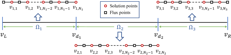
Figure 1: Illustration of the grid staggered by flux points and solution points for the case with two jumps at $v=v_{d_{1}}$ and $v=v_{d_{2}}$, respectively. The two jumps are both set to be solution points and used to divide the computational domain $[v_{{}_{L}},v_{{}_{R}}]$ into three subdomains $\Omega_{i}$ ($i=1,2,3$).

Given initial values at the solution points of the staggered grid, a finite difference scheme for Eq. (2) can be constructed by the following procedure:

1. Within each subdomain $\Omega_{i}$, obtain the solutions at the flux points by using interpolation schemes. For the purpose of stability, upwind interpolations are used here according to the sign of the drift $\Phi(v)$. If $\Phi(v)$ changes its sign within $\Omega_{i}$, we need to split the drift into an appropriate form to apply upwind interpolations. Here we split the drift into two parts: $\Phi(v)=\min\{\Phi(v),0\}+\max\{\Phi(v),0\}$, ensuring that each part does not change its sign. Then using this split form we can approximate the term $\Phi(v)p$ appearing in Eq. (2) at the flux point $v_{i,j+1/2}$ by

   $$\min \{\Phi(v_{i,j+1/2}),0\}p^{+}_{i,j+1/2}$$

   $$+\max\{\Phi(v_{i,j+1/2}),0\}p^{-}_{i,j+1/2},$$ (7)

   where $p^{+}_{i,j+1/2}$ and $p^{-}_{i,j+1/2}$ are the approximate values of $p$ at $v_{i,j+1/2}$, respectively, obtained by using interpolations with stencils as illustrated in Fig. 2;

2. Evaluate the first derivative of $p$ at flux points by using difference schemes in each subdomain $\Omega_{i}$;

3. Obtain the values of the current (3) at fluxes points by using the above two steps. Then approximate the values of the derivative of the current at solution points by using a difference scheme, which is designed for the domain $[v_{{}_{L}},v_{{}_{R}}]$ directly since the current (3) is theoretically continuous everywhere.

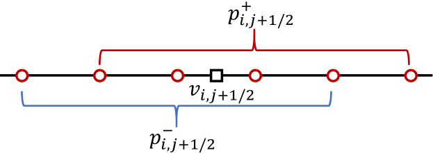
Figure 2: Illustration of the stencils used to reconstruct the values $p_{i,j+1/2}^{\pm}$ required by the approximation (7). Here only the stencils of the fifth-order interior interpolations are presented. Near the boundaries the stencils should be adjusted accordingly.

III Scheme

To discretize the right side of Eq. (2), we follow the aforementioned procedure: first calculate the values of the probability current at flux points and then derive a difference scheme to evaluate the derivative of the current. Here the spatial scheme is designed to be fifth-order for the cases with smooth drifts. Finally, a third-order Runge-Kutta scheme is employed to solve the resulting ordinary differential system.

III.1 Evaluation of the probability current

There are two terms appearing in the current (3). For the first term $\Phi(v)p$, we use interpolation schemes to reconstruct the required values in the approximation (7). For the second term $D\partial_{v}p$, we derive difference schemes to approximate it.

In the following, we will present the schemes in matrix forms, where the entries of the matrices are all easily obtained by using Lagrangian interpolations according to specified stencils. For example, if we consider the stencil $S=\{v_{1,1},v_{1,2},\dots,v_{1,5}\}$, then at any point $v$, the values of $p$ and $\partial_{v}p$ are approximated respectively by

$$p_{{}_{I}}(v)= \sum_{k=1}^{5}l_{k}(v)p_{1,k},$$ (8)

$$\frac{d}{dv}p_{{}_{I}}(v)= \sum_{k=1}^{5}\frac{d}{dv}l_{k}(v)p_{1,k},$$ (9)

where

$$l_{k}(v)=\prod_{s=1,s\neq k}^{5}\frac{v-v_{1,s}}{v_{1,k}-v_{1,s}}.$$ (10)

Since the grid points are slightly different in different subdomains (see Fig. 1), we describe the schemes separately for each subdomain $\Omega_{i}$. For convenience of notations, we will first consider the subdomain $\Omega_{2}$, and then $\Omega_{1}$ and $\Omega_{3}$.

III.1.1 Subdomain $\Omega_{2}$

To describe the scheme compactly, let us introduce the vectors $\mathbf{p}^{\pm}_{2}=[p^{\pm}_{2,3/2},p^{\pm}_{2,5/2},\dots,p^{\pm}_{2,N_{2}-1/2}]^{T}$ and the vector $\mathbf{p}_{2}=[p_{2,1},p_{2,2},\dots,p_{2,N_{2}}]^{T}$, where the “$T$” denotes the transpose operation. Then according to the grid point distribution in $\Omega_{2}$ we can compute the values at flux points by the fifth-order interpolation schemes $\mathbf{p}^{\pm}_{2}=I_{2}^{\pm}\mathbf{p}_{2}$, where $I_{2}^{\pm}$ are both $(N_{2}-1)\times N_{2}$ matrices. Here

$$I_{2}^{+}=\begin{bmatrix}\frac{35}{128}&\frac{35}{32}&-\frac{35}{64}&\frac{7}{32}&-\frac{5}{128}&&\\[3.0pt] -\frac{5}{128}&\frac{15}{32}&\frac{45}{64}&-\frac{5}{32}&\frac{3}{128}&&\\[3.0pt] &\ddots&\ddots&\ddots&\ddots&\ddots&\\[3.0pt] &&-\frac{5}{128}&\frac{15}{32}&\frac{45}{64}&-\frac{5}{32}&\frac{3}{128}\\[3.0pt] &&\frac{3}{128}&-\frac{5}{32}&\frac{45}{64}&\frac{15}{32}&-\frac{5}{128}\\[3.0pt] &&-\frac{5}{128}&\frac{7}{32}&-\frac{35}{64}&\frac{35}{32}&\frac{35}{128}\end{bmatrix},$$ (11)

and $I_{2}^{-}$ is defined by letting its entries satisfy that $[I_{2}^{-}]_{j,k}=[I_{2}^{+}]_{N_{2}-j,N_{2}+1-k}$, $1\leqslant j\leqslant N_{2}-1$, $1\leqslant k\leqslant N_{2}$.

Denote the approximation to $\partial_{v}p$ at the flux point $v_{2,j+1/2}$ as $(\partial_{v}p)_{2,j+1/2}$ and introduce the vector

$$\mathbf{p}_{2,v}=[(\partial_{v}p)_{2,3/2},(\partial_{v}p)_{2,5/2},\dots,(\partial_{v}p)_{2,N_{2}-1/2}]^{T}.$$

We can write the difference scheme as $\mathbf{p}_{2,v}=A_{2}\mathbf{p}_{2}/h_{2},$ where the $(N_{2}-1)\times N_{2}$ matrix $A_{2}$ is

$$A_{2}=\begin{bmatrix}-\frac{11}{12}&\frac{17}{24}&\frac{3}{8}&-\frac{5}{24}&\frac{1}{24}&&&\\[3.0pt] \frac{1}{24}&-\frac{9}{8}&\frac{9}{8}&-\frac{1}{24}&&&&\\[3.0pt] -\frac{3}{640}&\frac{25}{384}&-\frac{75}{64}&\frac{75}{64}&-\frac{25}{384}&\frac{3}{640}&&\\[3.0pt] &\ddots&\ddots&\ddots&\ddots&\ddots&\ddots&\\[3.0pt] &&-\frac{3}{640}&\frac{25}{384}&-\frac{75}{64}&\frac{75}{64}&-\frac{25}{384}&\frac{3}{640}\\[3.0pt] &&&&\frac{1}{24}&-\frac{9}{8}&\frac{9}{8}&-\frac{1}{24}\\[3.0pt] &&&-\frac{1}{24}&\frac{5}{24}&-\frac{3}{8}&-\frac{17}{24}&\frac{11}{12}\end{bmatrix},$$ (12)

such that the difference scheme is sixth-order at $v_{2,j+1/2}$ with $3\leqslant j\leqslant N_{2}-3$ and fourth-order at the other flux points.

III.1.2 Subdomain $\Omega_{1}$

Introduce $\mathbf{p}^{\pm}_{1}=[p^{\pm}_{1,1/2},p^{\pm}_{1,3/2},\dots,p^{\pm}_{1,N_{1}-1/2}]^{T}$ and $\mathbf{p}_{1}=[p_{1,1},p_{1,2},\dots,p_{1,N_{1}}]^{T}$. We first compute the right vector $\mathbf{p}^{+}_{1}$ by using the fifth-order interpolation scheme $\mathbf{p}^{+}_{1}=I_{1}^{+}\mathbf{p}_{1}$ with the $N_{1}\times N_{1}$ matrix $I_{1}^{+}$ written as

$$I_{1}^{+}=\begin{bmatrix}\mathbf{a}\\ (I_{2}^{+})_{(N_{1}-1)\times N_{1}}\end{bmatrix}.$$

Here

$$\mathbf{a}=\begin{bmatrix}\frac{315}{128}&-\frac{105}{32}&\frac{189}{64}&-\frac{45}{32}&\frac{35}{128}&0&\dots&0\end{bmatrix}$$ (13)

is a $1\times N_{1}$ vector and the matrix $(I_{2}^{+})_{(N_{1}-1)\times N_{1}}$ is defined in Eq. (11) by replacing $N_{2}$ with $N_{1}$ (The same notation method will be used throughout this paper). For the left values, first let $p^{-}_{1,1/2}=p^{+}_{1,1/2}$. Then we derive the interpolation scheme $\mathbf{p}^{-}_{1}=I_{1}^{-}[p^{-}_{1,1/2},\mathbf{p}_{1}^{T}]^{T}$ with the $N_{1}\times(N_{1}+1)$ matrix $I_{1}^{-}$ reading as

$$I_{1}^{-}=\begin{bmatrix}1&&&&&&&\\[3.0pt] -\frac{1}{7}&\frac{5}{8}&\frac{5}{8}&-\frac{1}{8}&\frac{1}{56}&&&\\[3.0pt] \frac{3}{35}&-\frac{1}{4}&\frac{3}{4}&\frac{9}{20}&-\frac{1}{28}&&&\\[3.0pt] &\frac{3}{128}&-\frac{5}{32}&\frac{45}{64}&\frac{15}{32}&-\frac{5}{128}&&\\[3.0pt] &&\ddots&\ddots&\ddots&\ddots&\ddots&\\[3.0pt] &&&\frac{3}{128}&-\frac{5}{32}&\frac{45}{64}&\frac{15}{32}&-\frac{5}{128}\\[3.0pt] &&&-\frac{5}{128}&\frac{7}{32}&-\frac{35}{64}&\frac{35}{32}&\frac{35}{128}\end{bmatrix}.$$ (14)

Introducing the vector

$$\mathbf{p}_{1,v}=[(\partial_{v}p)_{1,1/2},(\partial_{v}p)_{1,3/2},\dots,(\partial_{v}p)_{1,N_{1}-1/2}]^{T},$$

we can derive the difference scheme $\mathbf{p}_{1,v}=A_{1}\mathbf{p}_{1}/h_{1}$ with the $N_{1}\times N_{1}$ matrix $A_{1}$ written as

$$A_{1}=\begin{bmatrix}\mathbf{b}\\ (A_{2})_{(N_{1}-1)\times N_{1}}\end{bmatrix},$$

where

$$\mathbf{b}=\begin{bmatrix}-\frac{31}{8}&\frac{229}{24}&-\frac{75}{8}&\frac{37}{8}&-\frac{11}{12}&0&\dots&0\\ \end{bmatrix}$$ (15)

is a $1\times N_{1}$ vector and $A_{2}$ is defined in Eq. (12), such that the difference scheme is sixth-order at $v_{1,j+1/2}$ with $3\leqslant j\leqslant N_{1}-3$ and fourth-order at the other flux points.

III.1.3 Subdomain $\Omega_{3}$

The schemes for this subdomain are basically the same as those of the subdomain $\Omega_{2}$ if we swap the direction. Introduce $\mathbf{p}^{\pm}_{3}=[p^{\pm}_{3,3/2},p^{\pm}_{3,5/2},\dots,p^{\pm}_{3,N_{3}+1/2}]^{T}$ and $\mathbf{p}_{3}=[p_{3,1},p_{3,2},\dots,p_{3,N_{3}}]^{T}$. We first reconstruct the vector $\mathbf{p}^{-}_{3}$ by using the fifth-order interpolation scheme $\mathbf{p}^{-}_{3}=I_{3}^{-}\mathbf{p}_{3}$ with the entries of the $N_{3}\times N_{3}$ matrix $I_{3}^{-}$ defined by $[I_{3}^{-}]_{j,k}=[(I_{1}^{+})_{N_{3}\times N_{3}}]_{N_{3}+1-j,N_{3}+1-k}$. Then the right values are calculated by the fifth-order interpolation scheme $\mathbf{p}^{+}_{3}=I_{3}^{+}[\mathbf{p}_{3}^{T},p^{+}_{3,N_{3}-1/2}]^{T}$, where the entries of the $N_{3}\times(N_{3}+1)$ matrix $I_{3}^{+}$ are derived to be $[I_{3}^{+}]_{j,k}=[(I_{1}^{-})_{N_{3}\times(N_{3}+1)}]_{N_{3}+1-j,N_{3}+2-k}$. Note that we have assumed $p^{+}_{3,N_{3}-1/2}=p^{-}_{3,N_{3}-1/2}$ here.

Similarly, by introducing the vector

$$\mathbf{p}_{3,v}=[(\partial_{v}p)_{3,3/2},(\partial_{v}p)_{3,5/2},\dots,(\partial_{v}p)_{3,N_{3}+1/2}]^{T},$$

the derivative values at flux points are approximated by $\mathbf{p}_{3,v}=A_{3}\mathbf{p}_{3}/h_{3}$ with the entries of the $N_{3}\times N_{3}$ matrix $A_{3}$ defined by ${\color[rgb]{0,0,0}[A_{3}]_{j,k}=-[(A_{1})_{N_{3}\times N_{3}}]_{N_{3}+1-j,N_{3}+1-k}}$, such that the difference scheme is sixth-order at $v_{3,j+1/2}$ with $3\leqslant j\leqslant N_{3}-3$ and fourth-order at the other flux points.

III.1.4 Imposing boundary conditions

Using the above schemes derived for subdomains, we can obtain the values of the probability current at all flux points. However, it is noted that we have not used any boundary conditions so far. As we will see later in Sec. IV, depending on the signs of the drift at the domain boundaries we may need to set the computational domain to be large enough and impose reflecting boundary conditions Veestraeten2004 appropriately. In that cases, we just reset the current values at the boundaries to be zero.

III.2 Derivative of the current

Now we are ready to derive a difference scheme to compute the derivative of the current using the values at flux points obtained in Sec. III.1. To get a correct solution, it is no doubt that we have to consider information transmission between different subdomains $\Omega_{i}$. As mentioned before, although the derivative of the propagator is not continuous at jumps, the current is continuous everywhere. Therefore, we can derive a difference scheme for the whole domain directly to approximate the derivative of the current. However, as it allows different spatial steps in different subdomains, we have to pay attention to the solution points near the jumps.

For convenience of notations, let us introduce the flux vector $\mathbf{f}=[\mathbf{f}_{1}^{T},\mathbf{f}_{2}^{T},\mathbf{f}_{3}^{T}]^{T}$, where

$$\mathbf{f}_{1}=[f_{1,1/2},f_{1,3/2},\dots,f_{1,N_{1}-1/2}]^{T},$$ (16)

$$\mathbf{f}_{2}=[f_{2,3/2},f_{1,5/2},\dots,f_{2,N_{2}-1/2}]^{T},$$ (17)

$$\mathbf{f}_{3}=[f_{3,3/2},f_{1,5/2},\dots,f_{3,N_{3}+1/2}]^{T}.$$ (18)

The values of the derivative $\partial_{v}f$ at solution points are denoted by $\mathbf{f}_{v}=[\mathbf{f}_{1,v}^{T},\mathbf{f}_{2,v}^{T},\mathbf{f}_{3,v}^{T}]^{T}$ with

$$\mathbf{f}_{1,v}=[(\partial_{v}f)_{1,1},(\partial_{v}f)_{1,2},\dots,(\partial_{v}f)_{1,N_{1}}]^{T},$$ (19)

$$\mathbf{f}_{2,v}=[(\partial_{v}f)_{2,2},(\partial_{v}f)_{2,3},\dots,(\partial_{v}f)_{2,N_{2}}]^{T},$$ (20)

$$\mathbf{f}_{3,v}=[(\partial_{v}f)_{3,2},(\partial_{v}f)_{3,3},\dots,(\partial_{v}f)_{3,N_{3}}]^{T}.$$ (21)

Then we attempt to derive a derivative matrix $A$ such that $\mathbf{f}_{v}=A\mathbf{f}$. Here the size of $A$ is $N_{v}\times(N_{v}+1)$ with $N_{v}=N_{1}+N_{2}+N_{3}-2$.

By observing the distribution of the grid points, we design the difference scheme by using the stencils

$$[\mathbf{f}_{v}]_{j}=\begin{cases}\sum_{k=1}^{5}a_{j,k}[\mathbf{f}]_{k},&1\leqslant j\leqslant 2,\\[2.0pt] \sum_{k=1}^{6}a_{j,k}[\mathbf{f}]_{j+k-3},&3\leqslant j\leqslant N_{v}-2,\\[2.0pt] \sum_{k=1}^{5}a_{j,k}[\mathbf{f}]_{N_{v}+k-4},&N_{v}-1\leqslant j\leqslant N_{v},\\ \end{cases}$$ (22)

where $[\mathbf{f}]_{k}$ denotes the $k$-th entry of the vector $\mathbf{f}$ and the coefficients $a_{j,k}$ can be determined directly by using Lagrangian interpolations. Hence the difference matrix $A$ can be easily written down following the above stencils.

We first present the coefficients of the cases with stencils in a single subdomain. The results are as follows:

$$[a_{j,k}]_{1\leqslant k\leqslant 5} =\begin{cases}\frac{1}{h_{1}}[-\frac{11}{12},\frac{17}{24},\frac{3}{8},-\frac{5}{24},\frac{1}{24}],&j=1,\\[2.0pt] \frac{1}{h_{1}}[\frac{1}{24},-\frac{9}{8},\frac{9}{8},-\frac{1}{24},0],&j=2,\end{cases}$$ (23)

$$[a_{j,k}]_{1\leqslant k\leqslant 6} =\begin{cases}\frac{1}{h_{1}}\mathbf{c},&3\leqslant j\leqslant N_{1}-3,\\[2.0pt] \frac{1}{h_{2}}\mathbf{c},&N_{1}+3\leqslant j\leqslant N_{1}+N_{2}-4,\\[2.0pt] \frac{1}{h_{3}}\mathbf{c},&N_{1}+N_{2}+2\leqslant j\leqslant N_{v}-2,\end{cases}$$ (24)

$$[a_{j,k}]_{1\leqslant k\leqslant 5} =\begin{cases}\frac{1}{h_{3}}[0,\frac{1}{24},-\frac{9}{8},\frac{9}{8},-\frac{1}{24}],&j=N_{v}-1,\\[2.0pt] \frac{1}{h_{3}}[-\frac{1}{24},\frac{5}{24},-\frac{3}{8},-\frac{17}{24},\frac{11}{12}],&j=N_{v},\end{cases}$$ (25)

where the vector

$$\mathbf{c}=\begin{bmatrix}-\tfrac{3}{640}&\tfrac{25}{384}&-\tfrac{75}{64}&\tfrac{75}{64}&-\tfrac{25}{384}&\tfrac{3}{640}\end{bmatrix}.$$ (26)

For the other cases, we have to pay attention to the fact that the stencils (22) are across the jumps, as illustrated in Fig. 3. When $N_{1}-2\leqslant j\leqslant N_{1}+2$, by using Lagrangian interpolations we can determine the coefficients to be

$$a_{j,k}=d_{j-N_{1}+3,k}(h_{1},h_{2}),\quad 1\leqslant k\leqslant 6,$$ (27)

where $d_{s,k}(x,y)$ are functions of $x$ and $y$, as shown in Tab. 1. Similarly, when $N_{1}+N_{2}-3\leqslant j\leqslant N_{1}+N_{2}+1$, we have

$$a_{j,k}=d_{j-N_{1}-N_{2}+4,k}(h_{2},h_{3}),\quad 1\leqslant k\leqslant 6.$$ (28)

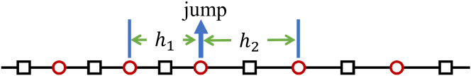
Figure 3: Illustration of the grid points near a jump. The spatial steps on the left and on the right of the jump are $h_{1}$ and $h_{2}$, respectively.

	$s=1$	$s=2$	$s=3$
$d_{s,1}(x,y)$	$-\frac{3}{64(9x+y)}$	$\frac{-8x^{2}-4xy+3y^{2}}{24x(7x+y)(7x+3y)}$	$\frac{60y^{3}-69xy^{2}}{20x(x+y)(5x+y)(5x+3y)}$
$d_{s,2}(x,y)$	$\frac{23x+2y}{336x^{2}+48xy}$	$\frac{16x^{2}+12xy-3y^{2}}{8x(5x+y)(5x+3y)}$	$\frac{5(23x-18y)y^{2}}{6x(x+y)(3x+y)(3x+5y)}$
$d_{s,3}(x,y)$	$-\frac{9(21x+4y)}{32x(5x+y)}$	$-\frac{88x^{2}+116xy+21y^{2}}{24x(x+y)(3x+y)}$	$\frac{15y^{2}(8y-23x)}{4x(x+y)(x+3y)(x+5y)}$
$d_{s,4}(x,y)$	$\frac{57x+18y}{48x^{2}+16xy}$	$\frac{32x^{2}+124xy+69y^{2}}{24x(x+y)(x+3y)}$	$\frac{15x^{2}(23y-8x)}{4y(x+y)(3x+y)(5x+y)}$
$d_{s,5}(x,y)$	$-\frac{17x+8y}{192x(x+y)}$	$-\frac{x^{3}(x+24y)}{y(x+y)(3x+y)(5x+y)(7x+y)}$	$\frac{5x^{2}(18x-23y)}{6y(x+y)(x+3y)(5x+3y)}$
$d_{s,6}(x,y)$	$\frac{18x^{4}}{(x+y)(3x+y)(5x+y)(7x+y)(9x+y)}$	$\frac{x^{3}(x+8y)}{3y(x+y)(x+3y)(5x+3y)(7x+3y)}$	$\frac{3x^{2}(23y-20x)}{20y(x+y)(x+5y)(3x+5y)}$

Table 1: Coefficients that determine the difference scheme (22) for the cases $N_{1}-2\leqslant j\leqslant N_{1}+2$ and $N_{1}+N_{2}-3\leqslant j\leqslant N_{1}+N_{2}+1$. When $s=4$ and $5$, the coefficients are determined by the relation $d_{s,j}(x,y)=-d_{6-s,7-j}(y,x)$ for $1\leqslant j\leqslant 6$.

III.3 Time-marching scheme

Approximating the right side of Eq. (2) by using the above finite difference scheme, we obtain a semi-discretized system, denoted by

$$\frac{d\mathbf{p}}{dt}=R(\mathbf{p},t),$$ (29)

where $\mathbf{p}$ stands for the vector of the unknowns at solution points, and $R(\mathbf{p},t)$ represents the right hand side term. Then many time-marching schemes can be used to solve this system. In this paper we employ a traditional third-order Runge-Kutta scheme, written as

$$\mathbf{p}^{n+1}=\mathbf{p}^{n}+\frac{1}{9}\tau(2K_{1}+3K_{2}+4K_{3}),$$ (30)

$$\begin{cases}K_{1}=R(\mathbf{p}^{n},t_{n}),\\ K_{2}=R(\mathbf{p}^{n}+\frac{1}{2}\tau K_{1},t_{n}+\frac{1}{2}\tau),\\ K_{3}=R(\mathbf{p}^{n}+\frac{3}{4}\tau K_{2},t_{n}+\frac{3}{4}\tau),\end{cases}$$ (31)

where $\mathbf{p}^{n}$ denotes the value of $\mathbf{p}$ at time $t_{n}$ and $\tau$ is the time step.

IV Numerical examples

In this section, some benchmark problems are solved numerically to show the validity of the algorithm presented above. The discrete $L^{2}$-norm error for the case with two jumps is defined by

$$L^{2}\mbox{ error}= \Bigg{[}\sum_{j=1}^{N_{1}-1}e_{1,j}^{2}h_{1}+\frac{1}{2}e_{1,N_{1}}^{2}(h_{1}+h_{2})+\sum_{j=2}^{N_{2}-1}e_{2,j}^{2}h_{2}$$

$$+\frac{1}{2}e_{2,N_{2}}^{2}(h_{2}+h_{3})+\sum_{j=2}^{N_{3}}e_{3,j}^{2}h_{3}\Bigg{]}^{1/2},$$ (32)

where $e_{i,j}=p_{i,j}-p(v_{i,j})$ are the errors between numerical results and exact solutions. In addition, the $L^{\infty}$-norm error is defined by

$$L^{\infty}\mbox{ error}=\max_{i,j}\{|e_{i,j}|\}.$$ (33)

For other cases, the errors are defined similarly. The numerical convergence rate is defined by

$$\mbox{rate}=-\ln(E_{M}/E_{N})/\ln(M/N),$$ (34)

where $E_{M}$ and $E_{N}$ are the errors corresponding to the cases with $M$ and $N$ solution points, respectively.

In numerical computations, the initial condition of Eq. (2) given by a delta function cannot be used directly. Instead, if an exact solution to Eq. (2) is available we choose the initial condition to be $p(v,\tau_{0}|v_{0},0)$ and start the computation from $t=\tau_{0}$. Here $\tau_{0}$ is a constant that can be chosen appropriately for the considered problems. Otherwise, the initial condition is set to be Gaussian,

$$p(v,\tau_{0}|v_{0},0)=\frac{1}{\sqrt{4\pi D\tau_{0}}}e^{-[v-v_{0}-\Phi(v_{0})\tau_{0}]^{2}/(4D\tau_{0})},$$ (35)

which mimics the delta function when $\tau_{0}$ is small. For convenience, $D=0.5$ and $\tau_{0}=0.01$ are chosen for all test cases in this section.

It should be noted that the proposed finite difference scheme can also be applied to solve problems with continuous drifts. In the following, we first show that the scheme is actually fifth-order for smooth cases. Then we pay attention to the cases with drift-admitting jumps, where a second-order convergence rate is observed.

IV.1 Smooth drifts

The following two examples are used to confirm that the scheme described in Sec. III is fifth-order for the cases with smooth drifts. Here $v_{d_{1}}=0$ and $v_{d_{2}}=1$ are used to divide all the computational domains (see Fig. 1) and the time step is set to be $\tau=0.01\min\{h_{1}^{2},h_{2}^{2},h_{3}^{2}\}$.

IV.1.1 Constant drift

When $\Phi(v)=\mu$ with $\mu$ being a constant, Eq. (1) corresponds to the Brownian motion with a constant drift, whose propagator is simply Gaussian,

$$p(v,t|v_{0},0)=\frac{1}{\sqrt{4\pi Dt}}e^{-(v-v_{0}-\mu t)^{2}/(4Dt)}.$$ (36)

Here $\mu=1$ and $v_{0}=0$ are chosen and the solution domain is truncated to be $[-5,10]$. While a zero current boundary condition is set for the left boundary, i.e., $f(-5,t|v_{0},0)=0$, no boundary condition is needed for the right due to the positiveness of the chosen $\mu$. The numerical results obtained in Tab. 2 show that for this smooth case the algorithm proposed in this paper achieves a fifth-order convergence rate approximately, while only approximately second-order for the Chang-Cooper scheme ChangCooper1970 (see Appendix A), which is one of the most popular schemes for solving Fokker-Planck equations. As we can see from Fig. 4, when $t=8$ the current is much large than zero at the right boundary. But the proposed scheme still produces a solution that matches with the exact solution. This means that the computational domain is not necessary to be large to avoid boundary refection here. It is no doubt that this property is very desirable in numerical simulations.

The current method
$N_{1}$	$N_{2}$	$N_{3}$	$N_{v}$	$L^{2}$ error	rate	$L^{\infty}$ error	rate
40	10	20	68	1.39E-03	–	1.94E-03
80	20	40	138	5.16E-05	4.66	5.21E-05	5.11
160	40	80	278	1.77E-06	4.82	1.46E-06	5.11
320	80	160	558	5.09E-08	5.09	4.04E-08	5.15
The Chang-Cooper scheme
–	–	–	$N_{v}$	$L^{2}$ error	rate	$L^{\infty}$ error	rate
–	–	–	68	6.73E-01	–	9.35E-01
–	–	–	138	2.50E-01	1.40	3.25E-01	1.49
–	–	–	278	3.80E-02	2.69	5.80E-02	2.46
–	–	–	558	1.02E-02	1.89	1.58E-02	1.87

Table 2: Accuracy test for Eq. (2) with $\Phi(v)=1$ at time $t=1$. The total number of solution points is $N_{v}=N_{1}+N_{2}+N_{3}-2$. The Chang-Cooper scheme for Eq. (2) with constant drift $\Phi(v)=\mu$ is presented in Appendix A. Here, the errors are computed according to Eqs. (32) and (33), and the rates are defined by Eq. (34).

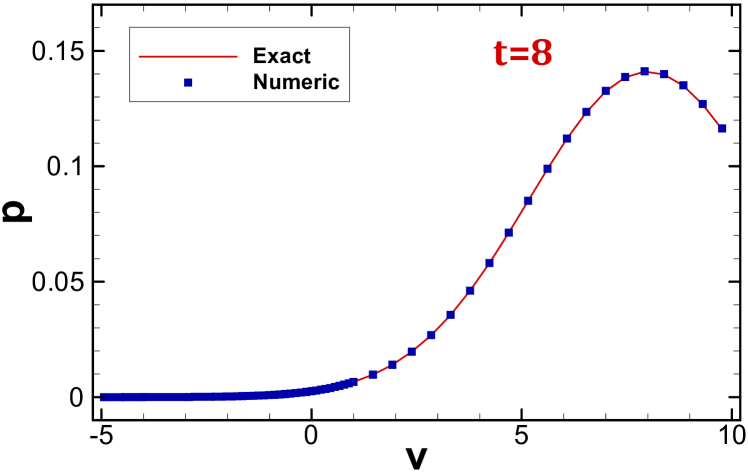
Figure 4: Numerical result of Eq. (2) with $\Phi(v)=1$ at time $t=8$. Here, $N_{1}=40$, $N_{2}=10$ and $N_{3}=20$ are used to compute the numerical result, which matches well with the exact solution (36).

IV.1.2 Ornstein-Uhlenbeck process

When $\Phi(v)=-\gamma v$ with $\gamma$ being a constant, Eq. (1) corresponds to the Ornstein-Uhlenbeck process. In this case, it is well known that Eq. (2) admits the solution

$$p(v,t|v_{0},0)=\sqrt{\frac{\gamma}{2\pi D(1-e^{-2\gamma t})}}\exp\left(-\frac{\gamma(v-e^{-\gamma t}v_{0})^{2}}{2D(1-e^{-2\gamma t})}\right).$$ (37)

For $\gamma>0$ and $t\rightarrow\infty$, the solution tends to the stationary solution

$$p_{{}_{\mathrm{OU}}}(v)=\sqrt{\frac{\gamma}{2\pi D}}e^{-\gamma v^{2}/(2D)}.$$ (38)

For $\gamma\leqslant 0$, no stationary solution exists.

Here we consider computations for the two cases $\gamma=1$ and $-1$. The computational domain $[-5,5]$ is chosen for both the cases. While zero current boundary conditions are set for the first case, no particular boundary condition is needed for the second. As we can see in Tab. 3 that the proposed scheme achieves fifth-order accuracy approximately for the two cases. Numerical results for larger time as shown in Fig. 5 confirm that the scheme is also valid for long time simulations, even for negative $\gamma$ without a large computational domain.

				$\gamma=1$
$N_{1}$	$N_{2}$	$N_{3}$	$N_{v}$	$L^{2}$ error	rate	$L^{\infty}$ error	rate
40	10	20	68	4.11E-04	–	3.93E-04	–
80	20	40	138	5.18E-05	2.93	5.63E-05	2.74
160	40	80	278	2.06E-06	4.60	2.03E-06	4.75
320	80	160	558	4.10E-08	5.62	3.86E-08	5.69
				$\gamma=-1$
$N_{1}$	$N_{2}$	$N_{3}$	$N_{v}$	$L^{2}$ error	rate	$L^{\infty}$ error	rate
40	10	20	68	3.29E-04	–	2.87E-04	–
80	20	40	138	5.59E-05	2.50	4.53E-05	2.61
160	40	80	278	2.34E-06	4.53	1.73E-06	4.67
320	80	160	558	4.75E-08	5.60	3.36E-08	5.65

Table 3: Accuracy test for Eq. (2) with $\Phi(v)=-\gamma v$ at time $t=0.5$ for two different values of $\gamma$. Here $N_{v}=N_{1}+N_{2}+N_{3}-2$. The errors are computed according to Eqs. (32) and (33), and the rates are defined by Eq. (34).

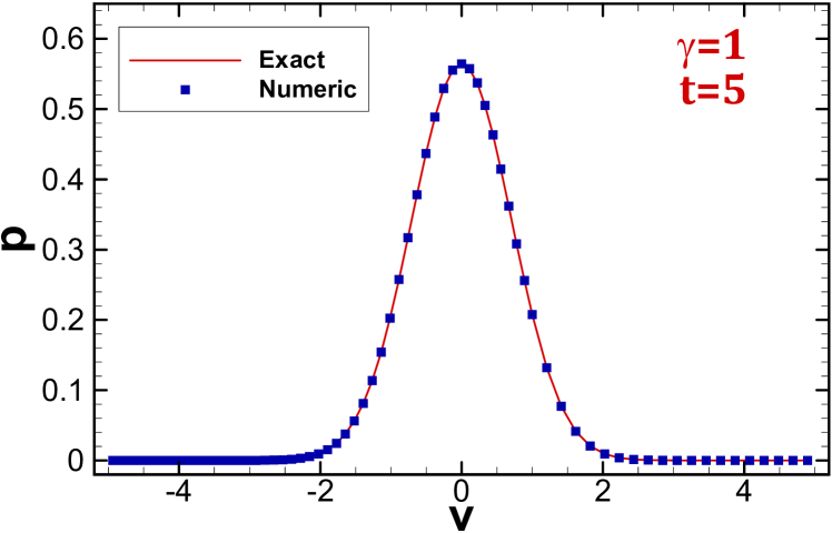
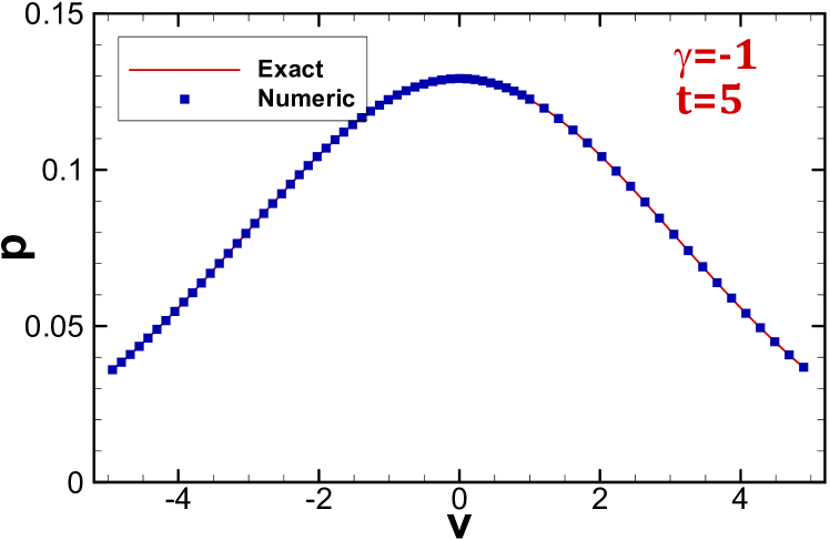
Figure 5: Numerical results of Eq. (2) with $\Phi(v)=-\gamma v$ for $\gamma=1$ and $\gamma=-1$ at different time. Here, $N_{1}=40$, $N_{2}=10$ and $N_{3}=20$ are used to compute the numerical results, which match well with the exact solution (37).

IV.2 Drifts admitting one jump

Since drifts admitting only one jump are considered, the computational domain is only divided into two subdomains by the jump here. Then we can modify the proposed finite difference scheme just by removing the subdomain $\Omega_{2}$ as shown in Fig. 1. Here the time step is chosen appropriately to be $\tau=0.01\min\{h_{1}^{2},h_{2}^{2}\}$.

IV.2.1 Pure dry friction

When $\Phi(v)=-\mu\,\text{sgn}(v)$ with $\mu$ being positive constant and “sgn” denoting the sign function, Eq. (1) corresponds to the Brownian motion with pure dry friction Gennes2005dryfriction , whose propagator is known in closed analytic form CaugheyDienes1961 ; Karatzas1984 ; TouchetteStraeten2010Brownian

$$p(v,t|v_{0},0)=\tfrac{\mu}{D}\hat{p}\left(\tfrac{\mu}{D}v,\tfrac{\mu^{2}}{D}t\big{|}\tfrac{\mu}{D}v_{0},0\right),$$ (39)

where

$$\hat{p}(x,\tau|x_{0},0)= \frac{e^{-\tau/4}}{2\sqrt{\pi\tau}}e^{-(|x|-|x_{0}|)/2}e^{-(x-x_{0})^{2}/(4\tau)}$$

$$+\frac{e^{-|x|}}{4}\left[1+\mathrm{erf}\left(\tfrac{\tau-(|x|+|x_{0}|)}{2\sqrt{\tau}}\right)\right]$$

with $\mathrm{erf}(x)=2\int_{0}^{x}\exp(-z^{2})dz/\sqrt{\pi}$ denoting the error function. The exact solution at time $t=\tau_{0}$ is set to be the initial condition with $v_{0}=2$, the computational domain is chosen to be $[-4,8]$ and zero current conditions are set at the boundaries. Figure 6 shows that the numerical results are consistent to the exact solutions. Since the solution admits a cusp at $v=0$ like peakons KalischRaynaud2006 , second-order accuracy is observed in Tab. 4, as expected. In addition, the results for a more general case with a two-valued drift are presented in Appendix B.

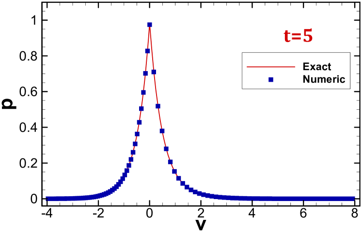
Figure 6: Propagators of Eq. (1) with the drift $\Phi(v)=-\mathrm{sgn}(v)$ at $t=1$ and $t=5$. Here $v_{0}=2$ and $N_{1}=N_{2}=50$ are chosen to compute the numerical results, which matches well with the exact solution (39).

$N_{1}$	$N_{2}$	$N_{v}$	$L^{2}$ error	rate	$L^{\infty}$ error	rate
50	50	99	4.73E-03	–	2.80E-03	–
100	100	199	1.21E-03	1.96	6.94E-04	2.00
200	200	399	3.01E-04	2.00	1.72E-04	2.00
400	400	799	7.57E-05	1.99	4.32E-05	1.99

Table 4: Accuracy test for Eq. (1) with the drift $\Phi(v)=-\mathrm{sgn}(v)$ at $t=1$. Here, $v_{0}=2$ and $N_{v}=N_{1}+N_{2}-1$. The errors are computed according to Eqs. (32) and (33), and the rates are defined by Eq. (34).

IV.2.2 Other drifts admitting one jump

Additional to the pure dry friction case, we consider here another two drifts admitting one jump, which are studied by using exact simulations of Eq. (1) in Etore2014 and papaspiliopoulos2016 , respectively.

The drift studied in Etore2014 is

$$\Phi(v)=\begin{cases}\frac{3\pi}{2}-\frac{\pi}{2}\cos\left(\frac{\pi}{5}v\right),&v<0,\\ -\frac{\pi}{2}\cos\left(\frac{\pi}{5}v\right),&v>0.\end{cases}$$ (40)

We choose the computational domain to be $[-2,3]$ and impose zero current conditions at the domain boundaries. The initial condition is set to be Eq. (35) with $v_{0}=0$. However, in Eq. (40) we did not define the value of $\Phi(0)$ since the proposed finite difference scheme does not involve the values of the drift at discontinuous points. Therefore, we have to define the value of $\Phi(0)$ involved in the initial condition (35). In this case, we define $\Phi(0)=[\Phi(0-)+\Phi(0+)]/2$. The same definition will be used throughout this paper. The profile of the numerical propagator as shown in Fig. 7(a) agrees with the result obtained in Etore2014 (see Fig. 4 therein). Moreover, the result obtained for a coarse grid matches with the fine-grid solution.

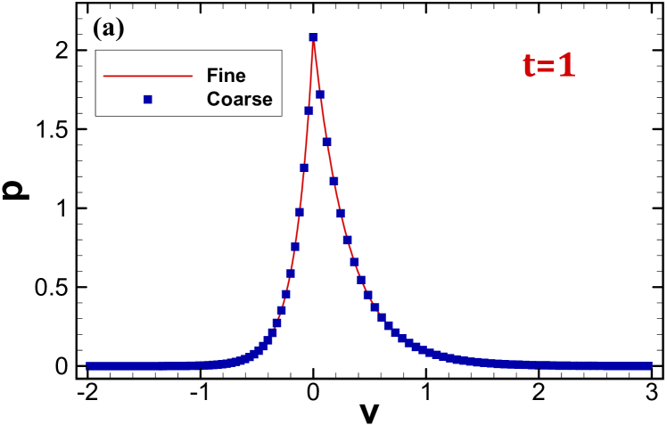
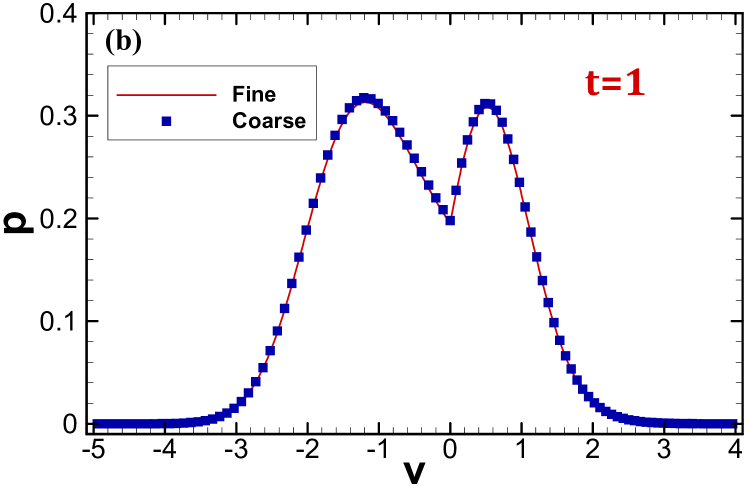
Figure 7: Propagators of Eq. (1) with the drifts (40) [(a)] and (41) [(b)] at $t=1$; $v_{0}=0$. Here the coarse-grid solutions obtained with $N_{1}=N_{2}=50$ match well with the fine-grid solutions obtained with $N_{1}=N_{2}=400$.

The drift investigated in papaspiliopoulos2016 is

$$\Phi(v)=\begin{cases}\sin\left(v-\tfrac{\pi}{4}\right),&v<0,\\ \sin\left(v-\tfrac{7\pi}{6}\right),&v>0.\end{cases}$$ (41)

The solution domain is truncated to be $[-5,4]$ and zero current conditions are imposed at the domain boundaries. As we can see from Fig. 7(b), the results agree with that obtained in papaspiliopoulos2016 (see Fig. 1 therein). Moreover, the results obtained by using a coarse grid and a fine grid match with each other.

IV.3 Drifts admitting two jumps

Here, the two examples presented in Dereudre2017 are considered. In both cases, the time step is chosen to be $\tau=0.01\min\{h_{1}^{2},h_{2}^{2},h_{3}^{2}\}$.

The first drift admitting two jumps reads as follows,

$$\Phi(v)=\begin{cases}0,&v<0,\\ 1,&0<v<1,\\ 0,&v>1,\end{cases}$$ (42)

which is piecewise-constant. In this case, the computational domain is chosen to be $[-4,6]$ and no numerical boundary condition is needed for the proposed scheme. The numerical solutions as shown in Fig. 8(a) agree with the result presented in Dereudre2017 (see Fig. 6(a) therein). In addition, the results obtained by using a coarse grid and a fine grid are consistent.

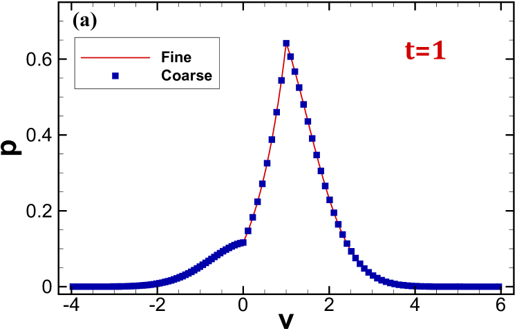
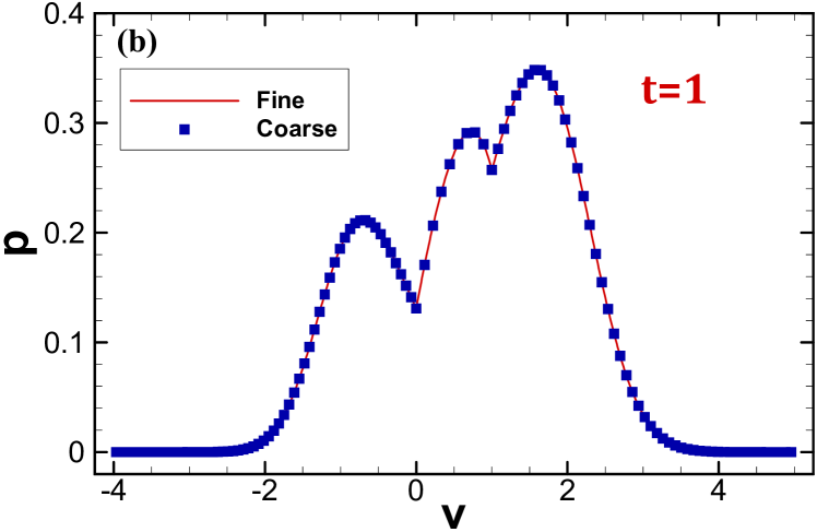
Figure 8: Propagators of Eq. (1) with the drift (42) at time $t=1$ [(a)] and the drift (43) at time $t=0.6$ [(b)]. Here, $v_{0}=0.5$ is chosen for both cases. The coarse-grid solutions are obtained with $N_{1}=60$, $N_{2}=10$ and $N_{3}=50$, and the fine-grid solutions are obtained with $N_{1}=480$, $N_{2}=80$ and $N_{3}=400$. The coarse-grid solutions match well with the fine-grid solutions.

The second drift is

$$\Phi(v)=\begin{cases}-2\cos(v),&v<0,\\ \sin(v),&0<v<1,\\ \cos(v-1)+\sin(1),&v>1.\end{cases}$$ (43)

The computational domain is chosen to be $[-4,5]$, which is large enough for us to impose zero current conditions at the domain boundaries for time $t=0.6$ with $v_{0}=0.5$. As shown in Fig. 8(b), the profile of the propagator agrees with that presented in Dereudre2017 (see Fig. 6(b) therein). Again, it is observed that the results obtained by using a coarse grid and a fine grid are consistent.

V Extension to functionals

Functionals of a stochastic process have been investigated intensively in the past and have found numerous applications in physics. Here we consider the functional

$$u(t)=\int_{0}^{t}K(v(s))ds$$ (44)

with an integrable kernel $K(v)$, where the stochastic process $v(t)$ obeys the Langevin equation (1). In particular, we have $u(0)=0$. The joint propagator of $u$ and $v$, denoted by $p=p(u,v,t|v_{0},0)$, is governed by the following Fokker-Planck equation

$$\partial_{t}\,p=-K(v)\partial_{u}\,p-\partial_{v}[\Phi(v)p]+\partial_{v}^{2}\,p$$ (45)

with the initial condition

$$p(u,v,0|v_{0},0)=\delta(u)\delta(v-v_{0}).$$ (46)

V.1 Scheme

To solve Eq. (45), we have to use the same matching conditions at the discontinuities of the drift $\Phi(v)$ (in the $v$ direction) as Eq. (2), while in the $u$ direction we just need to use the continuous condition as usual. Therefore, the scheme derived for Eq. (2) can be applied directly for the $v$ direction. In the $u$ direction, we choose the computational domain to be $[u_{{}_{L}},u_{{}_{R}}]$. Then a uniform staggered grid as shown in Fig. 9 is used. Here the flux points and solution points are

$$u_{k+1/2}=u_{{}_{L}}+kh_{u},\quad 0\leqslant k\leqslant N_{u},$$ (47)

$$u_{k}=u_{{}_{L}}+(k-1/2)h_{u},\quad 1\leqslant k\leqslant N_{u},$$ (48)

where $N_{u}$ denotes the number of solution points in the $u$ direction and the step $h_{u}=(u_{{}_{R}}-u_{{}_{L}})/N_{u}$.

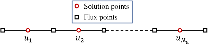
Figure 9: Illustration of the uniform grid staggered by flux points (47) and solution points (48) for the $u$ direction.

Similar to the approximation to the term $\Phi(v)p$ appearing in the current (3), we approximate the term $K(v)\partial_{u}p$ at the point $(u_{k},v_{j})$ by

$$\min\{K(v_{j}),0\}(\partial_{u}p)_{k,j}^{+}+\max\{K(v_{j}),0\}(\partial_{u}p)_{k,j}^{-},$$

where $(\partial_{u}p)_{k,j}^{+}$ and $(\partial_{u}p)_{k,j}^{-}$ are obtained by the following procedure. For a fixed $v_{j}$, we first reconstruct the values of the propagator at $u_{k+1/2}$ from the values at solution points by using fifth-order interpolations. Introducing the following two $(N_{u}+1)\times N_{u}$ interpolation matrices,

$$I_{u}^{-}=\begin{bmatrix}(\mathbf{a})_{1\times N_{u}}\\[3.0pt] (I_{3}^{-})_{N_{u}\times N_{u}}\end{bmatrix},\quad I_{u}^{+}=\begin{bmatrix}(I_{1}^{+})_{N_{u}\times N_{u}}\\[3.0pt] \widetilde{\mathbf{a}}\end{bmatrix},$$

where $\mathbf{a}$ is defined in Eq. (13) and $\widetilde{\mathbf{a}}$ is defined by letting its entries satisfy that $[\widetilde{\mathbf{a}}]_{1,j}=[\mathbf{a}_{1\times N_{u}}]_{1,N_{u}+1-j}$, we can express the reconstructions as $\mathbf{p}_{\bullet j}^{\pm}=I_{u}^{\pm}\mathbf{p}_{\bullet j},$ where the vectors $\mathbf{p}_{\bullet j}^{\pm}=[p_{1/2,j}^{\pm},p_{3/2,j}^{\pm},\dots,p_{N_{u}+1/2,j}^{\pm}]^{T}$ and $\mathbf{p}_{\bullet j}=[p_{1,j},p_{2,j},\dots,p_{N_{u},j}]^{T}$. Then we approximate the derivative $\partial_{u}p$ at solution points as $(\partial_{u}p)_{\bullet j}^{\pm}=A_{u}\mathbf{p}_{\bullet j}^{\pm}/h_{u},$ where the vectors $(\partial_{u}p)_{\bullet j}^{\pm}=[(\partial_{u}p)_{1,j}^{\pm},(\partial_{u}p)_{2,j}^{\pm},\dots,(\partial_{u}p)_{N_{u},j}^{\pm}]^{T}$ and the $N_{u}\times(N_{u}+1)$ difference matrix $A_{u}$ is defined by ${\color[rgb]{0,0,0}A_{u}=(A_{2})_{(N_{u}-1)\times N_{u}}}$ such that the difference scheme is sixth-order at $u_{k}$ with $3\leqslant k\leqslant N_{u}-2$ and fourth-order at the other solution points.

Here, the third-order Runge-Kutta scheme (30) is still used to solve the resulting ordinary differential system.

V.2 Displacement

Particularly, in this work we focus on the displacement $u(t)=\int_{0}^{t}v(s)ds$ associated with the Brownian motion with pure dry friction, i.e., $\Phi(v)=-\text{sgn}(v)$ and $K(v)=v$ are chosen for Eq. (45). Here the the computational domain in the $v$ direction is divided into two subdomains by $v=0$. We set the initial condition to be

$$p(u,v,\tau_{0}|v_{0},0)= \frac{1}{4\pi D\tau_{0}}e^{-(u-v_{0}\tau_{0})^{2}/(4D\tau_{0})}$$

$$\times e^{-(v-v_{0}-\Phi(v_{0})\tau_{0})^{2}/(4D\tau_{0})}$$ (49)

and start the computations at $t=\tau_{0}$ with $\tau_{0}$ chosen to be $0.01$. In addition, the time step is chosen to be $\tau=0.01\min\{h_{u},h_{1},h_{2}\}$.

As mentioned in the Introduction, for the Brownian motion with pure dry friction, analytic expressions of the first two moments of the displacement are available by solving a backward Komogorov equation ChenJust2014II or using the method based on the Pugachev-Sveshnikov equation Berezin2018 . For instance, when $v_{0}=0$ and $D=1$ we can inverse the expressions (70) and (73) in ChenJust2014II to obtain the first two moments as

$$M_{1}(t)= 0,$$ (50)

$$M_{2}(t)= \left[\tfrac{1}{8}t^{4}+\tfrac{5}{6}t^{3}-2t^{2}+6t-10\right]\text{erfc}\left(\tfrac{\sqrt{t}}{2}\right)$$

$$+\Big{[}64-\sqrt{\tfrac{t}{\pi}}\left(\tfrac{1}{4}t^{3}+\tfrac{7}{6}t^{2}-\tfrac{13}{3}t+10\right)\Big{]}e^{-t/4}$$

$$+10t-54,$$ (51)

where $\text{erfc}(x)$ is the complementary error function.

For different time $t$, computational domains can be chosen differently. For simplicity, the domain in the $v$ direction is fixed to be $[-6,6]$, while the domain for the $u$ direction is set to be dependent on time. To compute the results shown in Fig. 10, the computational domain $u\in[-10,10]$ is chosen for $t=0.1$ and $t=1$, $u\in[-15,15]$ for $t=2.5$, and $u\in[-30,30]$ for $t=5$. While zero current conditions are set at the domain boundaries in the $v$ direction, no particular boundary condition is needed in the $u$ direction. Numerical evolution of the joined propagator is shown in Fig. 10. In addition, the corresponding propagators of the displacement obtained by

$$p_{\text{dis}}(u_{k},t|0)= \sum_{j=1}^{N_{1}-1}p_{j,k}h_{1}+\frac{1}{2}p_{N_{1},k}(h_{1}+h_{2})$$

$$+\sum_{j=N_{1}+1}^{N_{1}+N_{2}-1}p_{j,k}h_{2}$$ (52)

are illustrated in Fig. 11. To confirm the correctness of the results, the first two moments of the displacement are computed numerically by

$$\widetilde{M}_{s}(t)=h_{u}\sum_{k=1}^{N_{u}}(u_{k})^{s}p_{\text{dis}}(u_{k},t|0),\quad s=1,2.$$ (53)

As shown in Fig. 12, the results agree with the analytical expressions (50) and (51), indicating the validity of the numerical method.

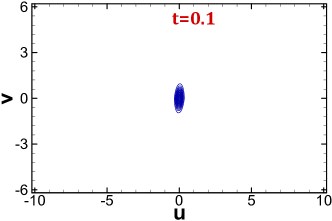
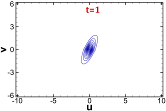
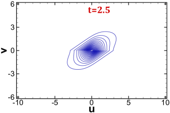
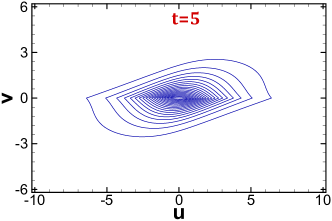
Figure 10: Contour plots of the joint propagator $p(u,v,t|v_{0},0)$ of Eq. (45) at different time with $\Phi(v)=-\text{sgn}(v)$, $K(v)=v$, $D=1$ and $v_{0}=0$. Here $N_{1}=N_{2}=100$ and $N_{u}=200$ are chosen to compute the numerical results.

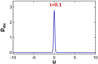
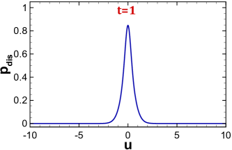
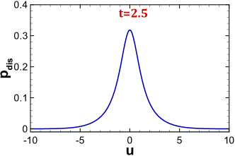
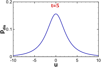
Figure 11: Propagators of the displacement (52) correspond to the numerical joint propagator $p(u,v,t|v_{0},0)$ at different time, as shown in Fig. 10.

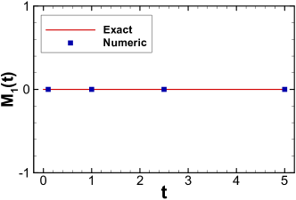
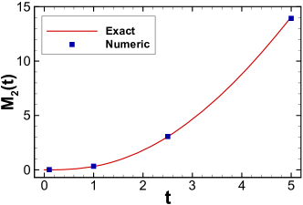
Figure 12: The first two moments of the displacement. Lines correspond to the exact solutions (50) and (51), and points to the numerical solutions obtained by using Eq. (53) for the displacement distributions as shown in Fig. 11.

VI Conclusions

We have derived in this paper a finite difference scheme to solve Fokker-Planck equations with drift-admitting jumps. The scheme is based on a grid staggered by flux points and solution points. In particular, the positions of the jumps are set to be solution points and used to split the solution domain into subdomains, such that we do not have to do much work to deal with the matching conditions of the propagator and the probability current at the jumps. Some benchmark problems have been computed numerically to show the validity of the scheme. The results showed that the scheme is fifth-order for the cases with smooth drifts and second-order for the cases with discontinuous drifts.

One of the desirable properties of the scheme is that, depending on the signs of the drift $\Phi(v)$ at the domain boundaries, we may not need to specify boundary conditions for the proposed scheme and could use a small computational domain to get a correct solution. This property is in particular useful when we extend the scheme to study functionals of a process, where no boundary condition is needed at the domain boundaries of the functionals. The displacement statistics of the Brownian motion with pure dry friction have been computed to show the effectiveness of the extended scheme.

The proposed numerical approach may be generalized to solve other problems involving discontinuous drifts, e.g., problems with both discontinuous drifts and some colored noises GeffertJust2017 , and high-dimensional problems with drift-admitting jumps DasPuri2017 .

Appendix A Chang-Cooper scheme for constant drift

Divide the computational interval $[v_{{}_{L}},v_{{}_{R}}]$ into $N$ cells with the nodes $v_{j}$ satisfying

$$v_{j}=v_{{}_{L}}+j\,h,\quad 0\leqslant j\leqslant N,$$ (54)

where the step $h=(v_{{}_{R}}-v_{{}_{L}})/N$. Then the Chang-Cooper scheme ChangCooper1970 for the Fokker-Planck equation (2) with the constant drift $\Phi(v)=\mu$ can be written as

$$\frac{1}{\tau}(p_{j}^{n+1}-p_{j}^{n})= \frac{1}{h}\frac{\mu}{1-e^{-\mu h/D}}(p_{j-1}^{n+1}-2p_{j}^{n+1}+p_{j+1}^{n+1})$$

$$-\frac{\mu}{h}(p_{j+1}^{n+1}-p_{j}^{n+1})$$ (55)

for $1\leqslant j\leqslant N-1$. Here $\tau$ is the time step. As stated in Sec. IV.1.1 for $\mu>0$, we impose zero boundary condition $p_{0}^{n+1}=0$ for all $n$. For $j=N$, we simply use an extrapolation scheme $p_{N}^{n+1}=2p_{N-1}^{n+1}-p_{N-2}^{n+1}$. Now introduce the vector $\mathbf{p}^{n}=[p_{1}^{n},p_{2}^{n},\dots,p_{N-1}^{n}]$, we can write the scheme (55) as a compact form $Z\mathbf{p}^{n+1}=\mathbf{p}^{n}$, where the matrix

$$Z=\begin{bmatrix}b&c\\ a&b&c\\ &\ddots&\ddots&\ddots\\ &&a&b&c\\ &&&a-c&b+2c\end{bmatrix}$$ (56)

with

$$a=\frac{\mu r}{\lambda-1},\;b=1-\mu r\frac{\lambda+1}{\lambda-1},\;c=\frac{\mu r\,\lambda}{\lambda-1}.$$ (57)

Here $r=\tau/h$ and $\lambda=e^{-\mu h/D}$.

Appendix B Two-valued drift

Let us consider in Eq. (1) the two-valued drift

$$\Phi(v)=\begin{cases}\mu_{{}_{L}},&v<0,\\ -\mu_{{}_{R}},&v>0,\end{cases}$$ (58)

where $\mu_{{}_{L}}$ and $\mu_{{}_{R}}$ are constants. Equation (1) with the drift (58) is called the Brownian motion with a two-valued drift, whose propagator can be expressed in terms of convolution integrals (see Eq. (5.7) in Karatzas1984 or Eq. (42) in SimpsonKuske2014TwoValued ). In the following, we consider three cases according to the signs of $\mu_{{}_{L}}$ and $\mu_{{}_{R}}$. Here the point $v=0$ is used to divide the computation domains into two subdomains and $\tau=0.01\min\{h_{1}^{2},h_{2}^{2}\}$ is chosen for the time step. In addition, we set the initial condition to be Eq. (35) with $\tau_{0}=0.01$ and start the computations from $t=\tau_{0}$.

B.1 Case 1: $\mu_{{}_{L}}>0$ and $\mu_{{}_{R}}>0$

For the case with $\mu_{{}_{L}}=\mu_{{}_{R}}>0$, this is just the Brownian motion with pure dry friction discussed in Sec. IV.2.1. Here $\mu_{{}_{L}}=1$ and $\mu_{{}_{R}}=2$ are chosen. The computational domain is set to be $[-3,3]$ and zero boundary conditions are imposed. The result shown in Fig. 13(a) demonstrates the validity of the numerical method for this case.

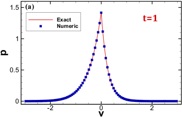
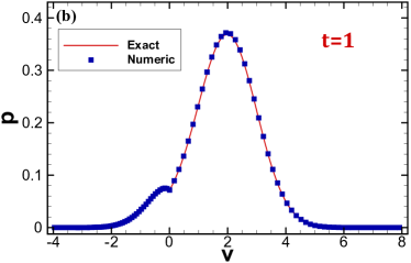
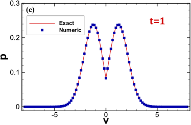
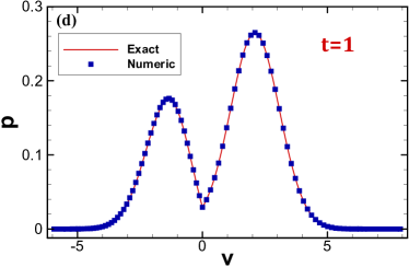
Figure 13: Propagators of the case (58) with different values of $\mu_{{}_{L}}$ and $\mu_{{}_{R}}$ at time $t=1$. Here $v_{0}=0$, $D=0.5$ and $N_{1}=N_{2}=50$ are chosen to compute the numerical solutions, which match well with the exact solutions that are obtained by evaluating the convolution integrals appearing in the analytic expression (see Eq. (5.7) in Karatzas1984 or Eq. (42) in SimpsonKuske2014TwoValued ) numerically by using the routine NIntegrate in Mathematica 8.0. (a) $\mu_{{}_{L}}=1$ and $\mu_{{}_{R}}=2$; (b) $\mu_{{}_{L}}=1$ and $\mu_{{}_{R}}=-2$; (c) $\mu_{{}_{L}}=-1$ and $\mu_{{}_{R}}=-1$; (d) $\mu_{{}_{L}}=-1$ and $\mu_{{}_{R}}=-2$.

B.2 Case 2: $\mu_{{}_{L}}>0$ and $\mu_{{}_{R}}<0$

In this case, when $\mu_{{}_{L}}=-\mu_{{}_{R}}=\mu>0$, Eq. (2) degenerates to the Brownian motion with a constant drift (see Sec. IV.1.1). For other cases with $\mu_{{}_{L}}\neq-\mu_{{}_{R}}$, it is expected that the propagator is nonsmooth at $v=0$. Here we consider the case with $\mu_{{}_{L}}=1$ and $\mu_{{}_{R}}=-2$. The computational domain is chosen to be $[-4,8]$, a zero current condition is set at the left boundary and no boundary condition is specified at the right. The numerical result as shown in Fig. 13(b) agrees with the exact solution, as expected.

B.3 Case 3: $\mu_{{}_{L}}<0$ and $\mu_{{}_{R}}<0$

In this case, no boundary condition is needed according to the signs of $\mu_{{}_{L}}$ and $\mu_{{}_{R}}$. For $v_{0}=0$ it is expected that the propagator is symmetric for $\mu_{{}_{L}}=\mu_{{}_{R}}$ and nonsymmetric for $\mu_{{}_{L}}\neq\mu_{{}_{R}}$. For $\mu_{{}_{L}}=\mu_{{}_{R}}=-1$, the computational domain $[-8,8]$ is used. The result depicted in Fig. 13(c) shows that the numerical result is consistent with the exact solution. For $\mu_{{}_{L}}=-1$ and $\mu_{{}_{R}}=-2$, the computational domain $[-6,8]$ is chosen. The result shown in Fig. 13(d) also confirms the validity of the numerical method.