State bounding for positive coupled differential - difference equations with bounded disturbances

Abstract: In this paper, the problem of finding state bounds is considered, for the first time, for a class of positive time-delay coupled differential-difference equations (CDDEs) with bounded disturbances. First, we present a novel method, which is based on nonnegative matrices and optimization techniques, for computing a like-exponential componentwise upper bound of the state vector of the CDDEs without disturbances. The main idea is to establish bounds of the state vector on finite-time intervals and then, by using the solution comparison method and the linearity of the system, extend to infinite time horizon. Next, by using state transformations, we extend the obtained results to a class of CDDEs with bounded disturbances. As a result, componentwise upper bounds, ultimate bounds and invariant set of the perturbed system are obtained. The feasibility of obtained results are illustrated through a numerical example.

1 Introduction

Coupled differential-difference equations (CDDEs) are dynamical systems, which include a differential equation coupled with a difference equation. Due to the fact that there are many systems in engineering such as electrical systems, fluid systems, neutral systems and so on, which are described by (or reformulated into) CDDEs, the stability problem for classes of CDDEs has attracted much research attention during the past decades [1, 2, 3, 4, 5, 6, 7, 8, 9, 10]. The most widely used method to this problem is based on the Lyapunov-Krasovskii functionals combining with linear matrix inequality technique (see [3, 4, 5, 7, 6] and the reference therein). Recent, by exploiting properties Metzler/Schur matrices combining with the comparison method, the authors [8], for the first time, presented another method and reported a new result on stability of a class of positive CDDEs with bounded time-varying delays. The topic on stability analysis of positive CDDEs by using the second method has gained an quickly increasing research attention in the recent years [9, 10, 11, 12, 13, 14].

Disturbances are usually unavoidable in practical engineering systems due to many reasons such as external noises, measurement errors, modeling inaccuracies, linear approximation and so on. In the presence of disturbances, in general, it is hard to achieve asymptotic stability for perturbed dynamical systems. However, under the assumption that disturbances are bounded by a known bound, the bounded-ness/the convergence within a bounded set can be guaranteed. Hence, the topic on state bounding/reachable set bounding/robust convergence for classes dynamical systems perturbed by unknown-but-bounded disturbances has been an important issue in control theory and has attracted significant research attention during the past decades [15, 16, 17, 27, 18, 28, 19, 20, 29, 21, 30, 31, 32, 22, 23, 24, 25, 26]. There are two commonly used approaches to this problem. For classes of linear systems whose matrices are constant, the most widely used approach is based on the Lyapunov method combining with linear matrix inequality technique [17, 18, 19, 20, 21, 22, 23, 24, 25, 26]. For classes of positive linear systems, the second widely used approach is based on properties of Metzler/Schur matrices combining with the solution comparison method [27, 28, 29, 30, 31, 32]. It is worthy to note that the second approach combining with the comparison method is also very useful for classes of nonlinear/time-varying systems which are bounded by positive linear systems [30, 31, 32].

By using the first approach, the authors [19] reported an result on reachable set bounding for a class of perturbed time-delay singular systems, which includes class of CDDEs as a special case. Later, some its extensions to more general classes of singular systems has also given in [23, 24]. However, so far, there has not been any result, which is obtained by using the second approach, on state bounding for positive CDDEs/singular systems with bounded disturbances. Motivated by this, in the paper, we study about the problem of finding state bounds for a class of positive CDDEs with bounded disturbances by using the second approach. We present a novel method to derive componentwise state bounds for the positive CDDEs with bounded disturbances,including three main steps: (i) finite-time convergence for linear positive systems; (ii) like-exponential componentwise upper bound for CDDEs without disturbances; and (iii) state bounding for CDDEs with bounded disturbances.

The paper is organized as follows. After the introduction, the problem statement and preliminaries are introduced in Section 2. The main results are given in Section 3. A numerical example with simulation results are given in Section 4. Finally, a conclusion is drawn in Section 5.

2 Problem statement and preliminaries

Notations: $\mathbb{R}^{n}(\mathbb{R}_{0,+}^{n},\mathbb{R}_{+}^{n})$ is the $n$-dimensional (nonnegative, positive) vector space; $e_{i}=[0_{1\times(i-1)}$ $1\ 0_{1\times(n-i)}]^{T}\in\mathbb{R}^{n}$ is the $i^{th}$-unit vector in $\mathbb{R}^{n}$; $l_{j}=[0_{1\times(j-1)}$ $1\ 0_{1\times(m-j)}]^{T}\in\mathbb{R}^{m}$ is the $j^{th}$-unit vector in $\mathbb{R}^{m}$; $\overline{1,n}=\{1,2,\cdots,n\}$; given three vectors $x=[x_{1}\ x_{2}\ \cdots\ x_{n}]^{T}\in\mathbb{R}^{n},$ $y=[y_{1}\ y_{2}\ \cdots\ y_{n}]^{T}\in\mathbb{R}^{n}$, $q=[q_{1}\ q_{2}\ \cdots\ q_{n}]^{T}\in\mathbb{R}_{0,+}^{n},$ two $n\times n$ matrices $A=[a_{ij}]$ and $B=[b_{ij}]$, the following notations will be used in our development: $x\prec y(\preceq y)$ means that $x_{i}<y_{i}(\leq y_{i}),\forall i\in\overline{1,n}$; $A\prec B(\preceq B)$ means that $a_{ij}<b_{ij}(\leq b_{ij}),\forall i,j\in\overline{1,n}$; $A$ is nonnegative if $0\preceq A$; $A$ is a Metzler matrix if $a_{ij}\geq 0,\forall i,j\in\overline{1,n},i\not=j$; $\mathcal{B}(0,q)=\{x\in\mathbb{R}^{n}_{0,+}:\ x\preceq q\}$ is an orthotope (hyperrectangle) in $\mathbb{R}^{n}_{0,+}$; $s(A)=\max\{Re(\lambda):\lambda\in\sigma(A)\}$ stands for the spectral abscissa of a matrix $A$; $\rho(A)=\max\{|\lambda|:\lambda\in\sigma(A)\}$ stands for the spectral radius of a matrix $A$. $A$ is a Schur matrix if $\rho(A)<1$; The computations, such as minimum, maximum of a set of finite vectors, limitation of a vector-valued function, etc., are understood in the component-wise sense.

Consider the linear CDDEs with bounded time-varying delays

$$\begin{split}\dot{x}(t)&=Ax(t)+By(t-h_{1}(t))+\omega(t),\ t\geq t_{0}\geq 0,\\ y(t)&=Cx(t)+Dy(t-h_{2}(t))+d(t),\end{split}$$ (1)

where $x(.)\in\mathbb{R}_{0,+}^{n}$, $y(.)\in\mathbb{R}_{0,+}^{m}$ are the state vectors. Matrices $A\in\mathbb{R}^{n\times n}$, $B\in\mathbb{R}_{0,+}^{n\times m}$, $C\in\mathbb{R}_{0,+}^{m\times n}$ and $D\in\mathbb{R}_{0,+}^{m\times m}$ are known. $D$ is assumed to be a Schur matrix. The disturbance vectors $\omega(.)\in\mathbb{R}_{0,+}^{n}$, $d(.)\in\mathbb{R}_{0,+}^{m}$ are unknown but assumed to be bounded by known bounds, i.e.,

$$0 \preceq\omega(t)\preceq\overline{\omega},\ \ \forall t\geq t_{0},$$ (2)

$$0 \preceq d(t)\preceq\overline{d},\ \ \forall t\geq t_{0},\vspace{-0.2cm}$$ (3)

where $\overline{\omega},\overline{d}$ are two known vectors. The unknown time-varying delays, $h_{1}(.)\in\mathbb{R}_{0,+}$, $h_{2}(.)\in\mathbb{R}_{0,+}$ are continuous, not necessary to be differential and are also assumed to be bounded, i.e.,

$$\max_{t\geq t_{0}}\max\{h_{1}(t),h_{2}(t)\}\leq h_{M},$$ (4)

where $h_{M}$ is a known constant. The initial condition of system (1) is given by $x(t_{0})=\psi(t_{0})$, $y(s)=\phi(s),\ s\in[t_{0}-\tau_{M},t_{0})$. The initial values $\psi(t_{0})$ and $\phi(.)$ are unknown but assumed to be bounded by known bounds, i.e.,

$$0 \preceq\psi(t_{0})\preceq\overline{\psi},$$ (5)

$$0 \preceq\phi(s)\preceq\overline{\phi},\ \forall s\in[t_{0}-h_{M},t_{0}),$$ (6)

where $\overline{\psi},\overline{\phi}$ are known nonnegative constant vectors. Let us denote by $x(t,t_{0},\psi,\phi,\omega)$ and $y(t,t_{0},\psi,\phi,d)$ the state vectors with the initial values ($\psi,\phi$) and disturbances $(\omega(t),d(t))$ of system (1).

The objective of this paper is to find as small as possible componentwise upper bounds of the state vectors of system (1). Concisely, we construct two decreasing vector-valued functions which are componentwise upper bounds of the two state vectors $x(t,t_{0},\psi,\phi,\omega)$ and $y(t,t_{0},\psi,\phi,d)$.

First, we recall the definition of positive system.

Definition 1:

([33]) System (1) is said to be positive if for any non-negative initial values, $\psi(t_{0})\succeq 0$, $\phi(s)\succeq 0,s\in[t_{0}-h_{M},t_{0})$, the state trajectories of system (1) satisfy that $x(t,t_{0},\psi,\phi,\omega)\succeq 0$ and $y(t,t_{0},\psi,\phi,d)\succeq 0$, for all $t\geq t_{0}$.

The following lemmas are needed for our development.

Lemma 1:

([34]). (i) Let $M\in\mathbb{R}^{n\times n}$ be a nonnegative matrix. Then, the following statements are equivalent: $(i_{1})$ $M$ is Schur stable; $(i_{2})$ $(M-I)q\prec 0$ for some $q\in\mathbb{R}_{+}^{n}$; $(i_{3})$ $(I-M)^{-1}\succeq 0$.
(ii) Let $M\in\mathbb{R}^{n\times n}$ be a Metzler matrix. Then, the following statements are equivalent: $(ii_{1})$ $M$ is Hurwitz stable; $(ii_{2})$ $Mq\prec 0$ for some $q\in\mathbb{R}_{+}^{n}$; $(ii_{3})$ $M^{-1}\preceq 0$.

Lemma 2:

([8, 10]) Assume that $A$ is a Metzler matrix, $B$, $C$, $D$ are nonnegative, $D$ is a Schur matrix. Then,

(i) System (1) is positive.

(ii) For $\psi_{1}(t_{0})\preceq\psi_{2}(t_{0})$ and $\phi_{1}(s)\preceq\phi_{2}(s),s\in[t_{0}-\tau_{M},t_{0})$, we have

$$x(t,t_{0},\psi_{1},\phi_{1},\omega) \preceq x(t,t_{0},\psi_{2},\phi_{2},\omega),\ \forall t\geq t_{0},$$ (7)

$$y(t,t_{0},\psi_{1},\phi_{1},d) \preceq y(t,t_{0},\psi_{2},\phi_{2},d),\ \forall t\geq t_{0}.$$ (8)

Lemma 3:

([35]) Assume that $A$ is a Metzler matrix, $B$, $C$, $D$ are nonnegative, Then, the following statements are equivalent
(i)  $\rho(D)<1$ and $s(A+B(I-D)^{-1}C)<0$;
(ii) there exist $p\in\mathbb{R}_{+}^{n}$, $q\in\mathbb{R}_{+}^{m}$ such that

$$Ap+Bq\prec 0,$$ (9)

$$Cp+(D-I)q\prec 0;$$ (10)

(iii) $s(A)<0$ and $\rho(C(-A)^{-1}B+D)<1$.

Remark 1:

Two matrix inequalities (9), (10) can be reformulated into the compact form
$\left[\begin{matrix}A&B\\ C&D-I\end{matrix}\right]\left[\begin{matrix}p\\ q\end{matrix}\right]\prec 0$. By (ii) of Lemma 1, we have $\left[\begin{matrix}A&B\\ C&D-I\end{matrix}\right]^{-1}\preceq 0$. Since matrix $\left[\begin{matrix}A&B\\ C&D-I\end{matrix}\right]^{-1}$ is non-singular and all its row vectors are non-zero. Hence, the vector $[p^{T}\ \ q^{T}]^{T}$ can be computed by the following equation

$$\left[\begin{matrix}p\\ q\end{matrix}\right]=-\left[\begin{matrix}A&B\\ C&D-I\end{matrix}\right]^{-1}\xi,$$ (11)

where $\xi\in\mathbb{R}^{n+m}_{+}$.

Remark 2:

The authors [8, 35] used inequalities (9), (10) in order to derive asymptotic stability conditions for CDDEs (1). By using the completeness of the Euclidean space $\mathbb{R}^{n}$, the authors [10] proposed tighter inequalities, (15), (16) and (17), and used these inequalities to analyze stability of CDDEs with unbounded time-delays. In the paper, we also use these tighter inequalities to derive our main results (componentwise upper bounds of system (1)). Hence, in the following, we re-state these inequalities and recall its proof. Assume that condition (i) of Lemma 3 holds. Then, by (iii) of Lemma 3, we have $s(A)<0$ which implies that $A^{-1}\preceq 0$ due to (ii) of Lemma 1. Left multiplying $A^{-1}$ on inequality (9), we obtain

$$-A^{-1}Bq\prec p.$$ (12)

Since $D$ is a Schur matrix and nonnegative, by (i) of Lemma 1, matrix $(I-D)^{-1}$ is nonnegative. Left multiplying $(I-D)^{-1}$ on inequality (10), we obtain

$$(I-D)^{-1}Cp\prec q.$$ (13)

Matrix inequality (10) is also rewritten as

$$Cp+Dq\prec q.$$ (14)

Since (12), (13) and (14) are strict inequalities, by using the completeness of the Euclidean space $\mathbb{R}^{n}$, there is a positive scalar $\mu\in(0,1)$ such that

$$-A^{-1}Bq \preceq(1-\mu)p\prec p,$$ (15)

$$(I-D)^{-1}Cp \preceq(1-\mu)q\prec q,$$ (16)

$$Cp+Dq \preceq(1-\mu)q\prec q.$$ (17)

These tighter inequalities (15), (16) and (17) will be key estimates for deriving main results in next section.

3 Main results

3.1 Finite-time convergence of linear positive systems

In this subsection, we present a method to find the smallest possible time which guarantees the finite-time convergence (i.e., all the state vectors starting from a given bounded set converges within another given bounded set after a finite time) of linear positive systems. The result is needed in establishing a componentwise upper bound of CDDEs with/without bounded disturbances in the Sections 3.2 and 3.3. Consider the following linear positive system

$$\begin{split}&\dot{u}(t)=Au(t),\ t\geq t_{0}\geq 0,\\ &u(t_{0})=\theta,\end{split}$$ (18)

where $u(t)\in\mathbb{R}^{n}_{0,+}$ is the state vector; $A\in\mathbb{R}^{n\times n}$ is a Metzler matrix; the initial value $\theta$ is unknown but assumed to be bounded by a known bound $\overline{\theta}$, i.e., $0\preceq\theta\preceq\overline{\theta}$. Let us denote by $u(t,t_{0},\theta)$ the solution of system (18).

The object of this subsection is, for a given nonnegative vector $\delta=[\delta_{1}\ \cdots\ \delta_{n}]^{T}\in\mathbb{R}^{n}_{0,+}$, to find as small as possible time $T\geq 0$ such that $u(t,t_{0},\theta)\preceq\delta,\ \forall t\geq t_{0}+T.$

A.1. Exponential componentwise estimate of linear positive system

Lemma 4:

Assume that $A$ is a Hurwitz stable. Then, there are a positive scalar $\alpha>0$ and a vector-value function $\beta(\overline{\theta})$ such that the following exponential componentwise estimate holds:

$$u(t,t_{0},\theta)\preceq\beta(\overline{\theta})e^{-\alpha(t-t_{0})},\ \forall t\geq t_{0}.$$ (19)

Proof:.

Since $A$ is Hurwitz stable, there exists a positive scalar $\alpha>0$ such that $A+\alpha I$ is Hurwitz stable. Note that $s(A^{T}+\alpha I)=s(A+\alpha I)$. Therefore, matrix $A^{T}+\alpha I$ is also Hurwitz stable. By (ii) of Lemma 1, there is a vector $v\succ 0$ such that

$$v^{T}(A+\alpha I)\prec 0.$$ (20)

Let us consider the following Lyapunov functional

$$V(t)=v^{T}e^{\alpha t}u(t).$$ (21)

By a simple computation, the derivative of $V$ along the solution $u(t,t_{0},\theta)$ is given as below

$$\dot{V}(t)=v^{T}(A+\alpha I)e^{\alpha t}u(t,t_{0},\theta)\leq 0,\ \forall t\geq t_{0},$$ (22)

which follows that $V(t)\leq V(t_{0}),\ \forall t\geq t_{0}$. Combining with $v\succ 0$, $u(t,t_{0},\theta)$ $\succeq 0,\ \forall t\geq t_{0}$ and $u(t_{0},t_{0},\theta)=\theta\preceq\overline{\theta}$, we have, for each $i\in\overline{1,n}$, that

$$v_{i}u_{i}(t,t_{0},\theta)e^{\alpha t} \leq v^{T}u(t,t_{0},\theta)e^{\alpha t}$$

$$\leq v^{T}u(t_{0},t_{0},\theta)e^{\alpha t_{0}}$$

$$\leq v^{T}e^{\alpha t_{0}}\overline{\theta},\ \ \forall t\geq t_{0},$$ (23)

which follows that

$$u_{i}(t,t_{0},\theta)\leq\frac{v^{T}\overline{\theta}}{v_{i}}e^{-\alpha(t-t_{0})},\ \forall t\geq t_{0}.$$ (24)

Set $\beta_{i}(v,\overline{\theta})=\frac{v^{T}\overline{\theta}}{v_{i}}$ and $\beta(v,\overline{\theta})=[\beta_{1}(v,\overline{\theta}),\cdots,\beta_{n}(v,\overline{\theta})]^{T}$. Then, from (24), we obtain a exponential componentwise estimate (19). The proof of Lemma 4 is completed. ∎

Remark 3:

For a fixed decay rate $\alpha$ satisfying $s(A^{T}+\alpha I)<0$. Let us denote by $\Omega$ the set of all vectors $v\succ 0$ such that inequality (20) holds, i.e.,

$$\Omega=\{v\in\mathbb{R}_{+}^{n}:(A^{T}+\alpha I)v\prec 0\}.$$ (25)

Then, by taking the minimum of the vector-value function $\beta(v,\overline{\theta})$ subject to $v\in\Omega$, i.e.,

$$\min_{v\in\Omega}\beta(v,\overline{\theta})=[\min_{v\in\Omega}\beta_{1}(v,\overline{\theta}),\cdots,\min_{v\in\Omega}\beta_{n}(v,\overline{\theta})]^{T},$$ (26)

we obtain the smallest exponential componentwise estimate with the fixed decay rate $\alpha$ of system (18) as below

$$u(t,t_{0},\theta)\preceq\Big{(}\min_{v\in\Omega}\beta(v,\overline{\theta})\Big{)}e^{-\alpha(t-t_{0})},\ \forall t\geq t_{0}.$$ (27)

Next, we present a method to find $\min_{v\in\Omega}\beta_{i}(v,\overline{\theta})$, $i\in\overline{1,n}$. For simplicity, we consider the case where $i=1$.

A.2. Minimization of partial factor $\beta_{1}(v,\overline{\theta})$

Let us denote

$$\Lambda=\{-(A^{T}+\alpha I)^{-1}r:r\in\ \mathbb{R}_{+}^{n}\}.$$ (28)

Then, from Lemma 1, we can verify that

$$\Omega=\Lambda,$$ (29)

which means that every vector $v\in\Omega$ has the following form

$$v=-(A^{T}+\alpha I)^{-1}r,$$ (30)

where $r\in\ \mathbb{R}_{+}^{n}$. By substituting (30) into formula $\beta_{1}(v,\overline{\theta})=\frac{v^{T}\overline{\theta}}{v_{1}}$ with some algebraic manipulations, $\beta_{1}(v,\overline{\theta}))$ is simplified into the following rational function of a vector variable $r$, which is denoted by $\Gamma_{1}(r)$,

$$\beta_{1}(v,\overline{\theta})=\frac{a_{1}r_{1}+a_{2}r_{2}+\cdots+a_{n}r_{n}}{b_{1}r_{1}+b_{2}r_{2}+\cdots+b_{n}r_{n}}\triangleq\Gamma_{1}(r).$$ (31)

Hence, the problem of finding $\min_{v\in\Omega}\beta_{1}(v,\overline{\theta})$ is equivalent to the problem of finding $\min_{r\in\ \mathbb{R}_{+}^{n}}\Gamma_{1}(r)$. Because $\mathbb{R}^{n}_{+}$ is an open set in $\mathbb{R}^{n}$, the minimum of function $\Gamma_{1}(r)$ subject to $r\in\mathbb{R}^{n}_{+}$ may not exist. Therefore, instead of finding the minimum, we find the infimum of function $\Gamma_{1}(r)$ subject to $r\in\mathbb{R}^{n}_{+}$.

Note that, by Lemma 1, matrix $-(A^{T}+\alpha I)^{-1}$ is non-negative and nonsingular. This follows that all row vectors of matrix $-(A^{T}+\alpha I)^{-1}$ are non-negative and non-zero. Combining with the non-negativeness of vector $\overline{\theta}$, we can verify that vector $a=[a_{1}\ a_{2}\ \cdots\ a_{n}]^{T}$ is non-negative and that vector $b=[b_{1}\ b_{2}\ \cdots\ b_{n}]^{T}$ is non-negative and non-zero. Set $J=\{j\in\overline{1,n}:b_{j}>0\}$, then by (Lemma 4 in Nam IEEE AC, 2016), we have

$$\inf_{r\in\mathbb{R}_{+}^{n}}\Gamma_{1}(r)=\min_{j\in J}\frac{a_{j}}{b_{j}}\triangleq\gamma_{1}.$$ (32)

Thus, the smallest exponential estimate with a fixed decay rate $\alpha$ of the $1^{th}$ partial state vector can be given as below:

$$u_{1}(t,t_{0},\theta)\leq\gamma_{1}e^{-\alpha(t-t_{0})},\ \forall t\geq t_{0},$$ (33)

where $\gamma_{1}$ is computed by formula (32).

A.3. Finite-time convergence

For a given scalar $\delta_{1}>0$, set

$$t^{1}_{\alpha}=\begin{cases}0&if\ \ \gamma_{1}\leq\delta_{1},\\ -\frac{1}{\alpha}\ln\frac{\delta_{1}}{\gamma_{1}}\ \ &if\ \ \gamma_{1}>\delta_{1}.\end{cases}$$ (34)

From formula (33) with a simple computation, we can verify that

$$u_{1}(t,t_{0},\theta)\leq\delta_{1},\ \forall t\geq t_{0}+t^{1}_{\alpha}.$$ (35)

Note that $s(A^{T}+\alpha I)$ is an increasing function with respect to variable $\alpha$. By using the one-dimensional search method, we find the suppremum $\alpha_{max}$ of scalars $\alpha>0$ such that $s(A^{T}+\alpha I)<0$. Hence, by increasing $\alpha$ gradually from $0$ to $\alpha_{max}$ with a chosen small step, for example 0.001, and comparing the times $t_{\alpha}^{1}$ computed by (34), we find

$$T^{1}=\min_{\alpha\in(0,\alpha_{max}]}t_{\alpha}^{1}.$$ (36)

Then, $T^{1}$ is the smallest time which guarantees that

$$u_{1}(t,t_{0},\theta)\leq\delta_{1},\ \forall t\geq t_{0}+T^{1}.$$ (37)

Similarly, for given scalars $\delta_{i}>0,i=2,\cdots,n$, we also compute the smallest times $T^{i},\ i=2,\cdots,n$ such that $u_{i}(t,t_{0},\theta)\leq\delta_{i},\ \forall t\geq t_{0}+T^{i}.$ Set

$$T=\max\{T^{1},T^{2},\cdots,T^{n}\}.$$ (38)

Then, $T$ is the smallest time, which guarantees that the state vector $u(t,t_{0},\theta)$ converges componentwisely within the ball $\mathbb{B}(0,\delta)$ after the finite-time $T$, i.e.,

$$u(t,t_{0},\theta)\preceq\delta,\ \forall t\geq t_{0}+T.$$ (39)

We have now summarized the above presented statements into the following theorem.

Theorem 1:

Assume that $A$ is a Metzler matrix and Hurwitz stable. Given two vectors $\overline{\theta}\in\mathbb{R}^{n}_{0,+}$, $\delta\in\mathbb{R}^{n}_{0,+}$. Then, all trajectories of system (18) converge componentwisely within the ball $\mathbb{B}(0,\delta)$ after the finite-time, $T$, computed by formula (38).

3.2 Componentwise bounds for positive CDDEs without disturbances

In this subsection, we present a new result on componentwise bound of system (1) for the case no disturbance, i.e., $\omega(t)\equiv d(t)\equiv 0$. For simplicity, we consider system (1) with $t_{0}=0$.

Theorem 2:

Assume that $A$ is a Metzler matrix, $B$, $C$, $D$ are nonnegative, $D$ is a Schur matrix and $s(A+B(I-D)^{-1}C)<0$. Then, there exist two positive vectors $p\in\mathbb{R}^{n}_{+}$, $q\in\mathbb{R}^{m}_{+}$, a scalar $\mu\in(0,1)$, a time $T^{*}\geq h_{M}$, such that, for $k=0,1,2,\cdots,$ the following estimates hold:

$$\begin{split}x(t,0,\psi,\phi,0)&\preceq(1-\mu)^{k}p,\ \ \forall t\in[kT^{*},(k+1)T^{*}),\\ y(t,0,\psi,\phi,0)&\preceq(1-\mu)^{k+1}q,\ \ \forall t\in[kT^{*},(k+1)T^{*}).\end{split}$$ (40)

Proof:.

Step 1: By Lemma 3, Remark 1, there exist two vectors $\widetilde{p}\in\mathbb{R}^{n}_{+}$, $\widetilde{q}\in\mathbb{R}^{m}_{+}$ such that three inequalities (12), (13), (14) hold. For given two vectors $\overline{\psi}\in\mathbb{R}^{n}_{+}$, $\overline{\phi}\in\mathbb{R}^{m}_{+}$, set $\varrho=\max\{\frac{\overline{\psi}_{1}}{\widetilde{p}_{1}},\cdots,\frac{\overline{\psi}_{n}}{\widetilde{p}_{n}},\frac{\overline{\phi}_{1}}{\widetilde{q}_{1}},\cdots,\frac{\overline{\phi}_{m}}{\widetilde{q}_{m}}\}$, and choose $p=\varrho\widetilde{p}$, $q=\varrho\widetilde{q}$. Then, $p\succeq\overline{\psi}$, $q\succeq\overline{\phi}$ and (12), (13), (14) hold. By using one-dimensional search, we find a scalar $\mu\in(0,1)$ such that inequalities (15), (16), (17) hold. By (ii) of Lemma 2, we have

$$\begin{split}x(t,0,\psi,\phi,0)&\preceq x(t,0,p,q,0),\ \forall t\geq 0,\\ y(t,0,\psi,\phi,0)&\preceq y(t,0,p,q,0),\ \forall t\geq 0.\end{split}$$ (41)

Step 2: Next, we prove that there exist a time $T>0$ such that such that

$$\begin{split}x(t,0,p,q,0)&\preceq(1-\mu)p,\ \forall t\geq T,\\ y(t,0,p,q,0)&\preceq(1-\mu)^{2}q,\ \forall t\geq T,\end{split}$$ (42)

where $p,q$ $\mu$ are computed in Step 1. Indeed, let us consider the linear positive system

$$\dot{u}(t) =Au(t),\ \forall t\geq 0,$$ (43)

and by using Step 1 of the proof of Theorem 1 in [10] and (15), (16), (17), we obtain

$$x(t,0,p,q,0)\preceq p,\ \forall t\geq 0,$$ (44)

$$y(t,0,p,q,0)\preceq(1-\mu)q,\ \forall t\geq 0,$$ (45)

and the following solution comparison

$$x(t,0,p,q,0)\preceq-A^{-1}Bq+u(t,0,p+A^{-1}Bq),\forall t\geq 0,$$ (46)

By using Theorem 1 for system (43) with $\overline{\theta}=p+A^{-1}Bq$ and $\delta=(1-\mu)p+A^{-1}Bq$, we find the smallest time $T$ such that

$$u(t,0,p+A^{-1}Bq) \preceq(1-\mu)p+A^{-1}Bq,\forall t\geq T,$$ (47)

which follows that

$$x(t,0,p,q,0)\preceq(1-\mu)p,\forall t\geq T.$$ (48)

Set $T^{*}=\max\{T,h_{M}\}$. Then, from (45) and (48), we have

$$\begin{split}&x(t,0,p,q,0)\preceq(1-\mu)p,\ \ \forall t\geq T^{*}\\ &y(t,0,p,q,0)\preceq(1-\mu)q,\ \ \forall t\geq T^{*}-h_{M}.\end{split}$$ (49)

On the other hand, from (1), we have

$$y(t)=\begin{cases}Cx(t)+Dy(t-h_{2}(t))&\ \text{if}\ \ h_{2}(t)>0\\ (I-D)^{-1}Cx(t)&\ \text{if}\ \ h_{2}(t)=0.\end{cases}$$ (50)

Combining (16), (17), (49) and (50), we obtain

$$y(t,0,p,q,0)\preceq(1-\mu)^{2}q,\ \ \forall t\geq T^{*}.$$ (51)

From (44) and (45), we obtain inequality (40) for the case where $k=0$. From (49) and (51), we obtain inequality (40) for the case where $k=1$.

Step 3: In this step, we prove that inequality (40) hold for the case where $k=2$. In deed, let us consider the following system with the initial time $t_{0}=T^{*}$,

$$\begin{split}\dot{x}^{1}(t)&=Ax^{1}(t)+By^{1}(t-h_{1}(t)),\ t\geq T^{*}\geq 0,\\ y^{1}(t)&=Cx^{1}(t)+Dy^{1}(t-h_{2}(t)).\end{split}$$ (52)

Similar to Step 2, we also prove that

$$\begin{split}x^{1}(t,T^{*},p,q,0)&\preceq(1-\mu)p,\ \forall t\in[2T^{*},3T^{*}),\\ y^{1}(t,T^{*},p,q,0)&\preceq(1-\mu)^{2}q,\ \forall t\in[2T^{*},3T^{*}).\end{split}$$ (53)

By using the linearity of system (52), from (53), we also obtain, for any positive scalar $\lambda$, that

$$\begin{split}x^{1}(t,T^{*},\lambda p,\lambda q,0)&\preceq(1-\mu)\lambda p,\ \ \forall t\in[2T^{*},3T^{*}),\\ y^{1}(t,T^{*},\lambda p,\lambda q,0)&\preceq(1-\mu)^{2}\lambda q,\ \ \forall t\in[2T^{*},3T^{*}).\end{split}$$ (54)

Choosing $\lambda=1-\mu$ and from (54), we have

$$\begin{split}x^{1}(t,T^{*},(1-\mu)p,(1-\mu)q,0)&\preceq(1-\mu)^{2}p,\ \ \forall t\in[2T^{*},3T^{*}),\\ y^{1}(t,T^{*},(1-\mu)p,(1-\mu)q,0)&\preceq(1-\mu)^{3}q,\ \ \forall t\in[2T^{*},3T^{*}).\end{split}$$ (55)

On the other hand, inequality (49) implies that, we have

$$\begin{split}&x(T^{*},0,p,q,0)\preceq(1-\mu)p,\\ &y(t,0,p,q,0)\preceq(1-\mu)q,\ \ \forall t\in[T^{*}-h_{M},T^{*}).\end{split}$$ (56)

Combining with part (ii) of Lemma 2, we have

$$\begin{split}x(t,0,p,q,0)&\preceq x^{1}(t,T^{*},(1-\mu)p,(1-\mu)q,0),\ \forall t\geq T^{*},\\ y(t,0,p,q,0)&\preceq y^{1}(t,T^{*},(1-\mu)p,(1-\mu)q,0),\ \forall t\geq T^{*}.\end{split}$$ (57)

From (55) and (57), we obtain

$$\begin{split}x(t,0,p,q,0)&\preceq(1-\mu)^{2}p,\ \ \forall t\in[2T^{*},3T^{*}),\\ y(t,0,p,q,0)&\preceq(1-\mu)^{3}q,\ \ \forall t\in[2T^{*},3T^{*}).\end{split}$$ (58)

This means that we have inequality (40) for the case where $k=2$. By doing similarly as above, we also obtain inequality (40) for the cases where $k=3,4,\cdots.$ The proof of Theorem 2 is completed. ∎

3.3 Componentwise bounds for positive CDDEs perturbed by bounded disturbances

This subsection is to extend the above obtained result to class of CDDEs perturbed by bounded-nonzero-disturbances. For simplicity, we consider also system (1) with $t_{0}=0$.

Theorem 3:

Assume that conditions given in Theorem 2 hold. Set

$$\left[\begin{matrix}\eta\\ \varsigma\end{matrix}\right]=-\left[\begin{matrix}A&B\\ C&D-I\end{matrix}\right]^{-1}\left[\begin{matrix}\overline{\omega}\\ \overline{d}\end{matrix}\right].$$ (59)

(i) There exist two positive vectors $p\in\mathbb{R}^{n}_{+}$, $q\in\mathbb{R}^{m}_{+}$, a scalar $\mu\in(0,1)$, a time $T^{*}\geq h_{M}$, such that, for $k=0,1,2,\cdots,$ the following exponential componentwise estimates hold:

$$\begin{split}x(t,0,\psi,\phi,\omega)&\preceq\eta+(1-\mu)^{k}p,\ \ \forall t\in[kT^{*},(k+1)T^{*}),\\ y(t,0,\psi,\phi,d)&\preceq\varsigma+(1-\mu)^{k+1}q,\ \ \forall t\in[kT^{*},(k+1)T^{*}).\end{split}$$ (60)

(ii) The vector $\left[\begin{matrix}\eta\\ \varsigma\end{matrix}\right]$ is the smallest componentwise ultimate bound of system (1).

(iii) The ball $\mathbb{B}\left(0,\left[\begin{matrix}\eta\\ \varsigma\end{matrix}\right]\right)$ is the smallest invariant set, which is different from $\{0\}$, of system (1).

Proof:.

(i)  Let us consider the following system:

$$\begin{split}\dot{\overline{x}}(t)&=A\overline{x}(t)+B\overline{y}(t-h_{1}(t))+\overline{\omega},\ t\geq 0,\\ \overline{y}(t)&=C\overline{x}(t)+D\overline{y}(t-h_{2}(t))+\overline{d}.\end{split}$$ (61)

Set $\left[\begin{matrix}\widehat{\psi}\\ \widehat{\phi}\end{matrix}\right]=\max\left\{\left[\begin{matrix}\overline{\psi}\\ \overline{\phi}\end{matrix}\right],\left[\begin{matrix}\eta\\ \varsigma\end{matrix}\right]\right\}.$ By both (i) and (ii) of Lemma 2, we have

$$\begin{split}x(t,0,\psi,\phi,\omega)&\preceq\overline{x}(t,0,\widehat{\psi},\widehat{\phi},\overline{\omega}),\ \ t\geq 0,\\ y(t,0,\psi,\phi,d)&\preceq\overline{y}(t,0,\widehat{\psi},\widehat{\phi},\overline{d}),\ \ t\geq 0.\end{split}$$ (62)

Taking the following state transformation

$$\begin{split}\check{x}(t)&=\overline{x}(t)-\eta,\\ \check{y}(t)&=\overline{y}(t)-\varsigma,\end{split}$$ (63)

then, we have

$$\begin{split}\dot{\check{x}}(t)&=A\check{x}(t)+B\check{y}(t-h_{1}(t)),\ t\geq 0,\\ \check{y}(t)&=C\check{x}(t)+D\check{y}(t-h_{2}(t)),\end{split}$$ (64)

and

$$\begin{split}\check{x}(t,0,\widehat{\psi}-\eta,\widehat{\phi}-\varsigma,0)&=\overline{x}(t,0,\widehat{\psi},\widehat{\phi},\overline{\omega})-\eta,\\ \check{y}(t,0,\widehat{\psi}-\eta,\widehat{\phi}-\varsigma,0)&=\overline{y}(t,0,\widehat{\psi},\widehat{\phi},\overline{d})-\varsigma,\end{split}$$ (65)

Now, we apply Theorem 2 for system (64) with the initial values $(\widehat{\psi}-\eta,\widehat{\phi}-\varsigma)$, there exist two positive vectors $p,q$, a scalar $\mu\in(0,1)$ and the time $T^{*}\geq h_{M}$ such that, for $k=0,1,2,\cdots,$

$$\begin{split}\check{x}(t,0,\widehat{\psi}-\eta,\widehat{\phi}-\varsigma,0)&\preceq(1-\mu)^{k}p,\ \ \forall t\in[kT^{*},(k+1)T^{*}),\\ \check{y}(t,0,\widehat{\psi}-\eta,\widehat{\phi}-\varsigma,0)&\preceq(1-\mu)^{k+1}q,\ \ \forall t\in[kT^{*},(k+1)T^{*}).\end{split}$$ (66)

From (62), (65) and (66), we obtain inequalities (60).

(ii) From (60), by letting $t$ tend to infinity, we obtain,

$$\begin{split}\lim\sup_{t\rightarrow\infty}x(t,0,\psi,\phi,\omega)&\preceq\eta,\\ \lim\sup_{t\rightarrow\infty}y(t,0,\psi,\phi,d)&\preceq\varsigma.\end{split}$$ (67)

This follows that the vector $\left[\begin{matrix}\eta\\ \varsigma\end{matrix}\right]$ is a componentwise ultimate bound of system (1). In order to prove that the vector $\left[\begin{matrix}\eta\\ \varsigma\end{matrix}\right]$ is the smallest componentwise ultimate bound, we consider the case where $\omega(t)\equiv\overline{\omega}$ and $d(t)\equiv\overline{d}$ and take the following state transformation:

$$\begin{split}\widetilde{x}(t)&=\eta-x(t),\\ \widetilde{y}(t)&=\varsigma-y(t),\end{split}$$ (68)

then, from (1), we obtain

$$\begin{split}\dot{\widetilde{x}}(t)&=A\widetilde{x}(t)+B\widetilde{y}(t-h_{1}(t)),\ t\geq 0,\\ \widetilde{y}(t)&=C\widetilde{x}(t)+D\widetilde{y}(t-h_{2}(t)),\end{split}$$ (69)

and

$$\begin{split}\widetilde{x}(t,0,\eta,\varsigma,0)&=\eta-x(t,0,0,0,\overline{\omega}),\\ \widetilde{y}(t,0,\eta,\varsigma,0)&=\varsigma-y(t,0,0,0,\overline{d}).\end{split}$$ (70)

Now, we apply Theorem 2 for system (69) with the initial values $(\eta,\varsigma)$, there exist two positive vectors $p,q$, a scalar $\mu\in(0,1)$ and the time $T^{*}\geq h_{M}$ such that, for $k=0,1,2,\cdots,$

$$\begin{split}\widetilde{x}(t,0,\eta,\varsigma,0)&\preceq(1-\mu)^{k}p,\ \ \forall t\in[kT^{*},(k+1)T^{*}),\\ \widetilde{y}(t,0,\eta,\varsigma,0)&\preceq(1-\mu)^{k+1}q,\ \ \forall t\in[kT^{*},(k+1)T^{*}).\end{split}$$ (71)

From (70), (71), we have

$$\begin{split}\eta-(1-\mu)^{k}p&\preceq x(t,0,0,0,\overline{\omega}),\ \ \forall t\in[kT^{*},(k+1)T^{*}),\\ \varsigma-(1-\mu)^{k+1}q&\preceq y(t,0,0,0,\overline{d}),\ \ \forall t\in[kT^{*},(k+1)T^{*}).\end{split}$$ (72)

Letting $t$ tend to infinity, we obtain

$$\begin{split}\eta&\preceq\lim\inf_{t\rightarrow\infty}x(t,0,0,0,\overline{\omega}),\\ \varsigma&\preceq\lim\inf_{t\rightarrow\infty}y(t,0,0,0,\overline{d}).\end{split}$$ (73)

This implies that the vector $\left[\begin{matrix}\eta\\ \varsigma\end{matrix}\right]$ is the smallest componentwise ultimate bound.

(iii) For the case where $\left[\begin{matrix}\overline{\psi}\\ \overline{\phi}\end{matrix}\right]=\left[\begin{matrix}\eta\\ \varsigma\end{matrix}\right]$, then $\left[\begin{matrix}\widehat{\psi}\\ \widehat{\phi}\end{matrix}\right]=\left[\begin{matrix}\eta\\ \varsigma\end{matrix}\right]$. Substituting this equality into (65), we obtain

$$\begin{split}\overline{x}(t,0,\widehat{\psi},\widehat{\phi},\overline{\omega})\equiv\eta,\\ \overline{y}(t,0,\widehat{\psi},\widehat{\phi},\overline{d})\equiv\varsigma.\end{split}$$ (74)

Combining with (62), we obtain

$$\begin{split}x(t,0,\psi,\phi,\omega)&\preceq\eta,\ \ t\geq 0,\\ y(t,0,\psi,\phi,d)&\preceq\varsigma,\ \ t\geq 0,\end{split}$$ (75)

From (73) and (75), we conclude that the ball $\mathbb{B}\left(0,\left[\begin{matrix}\eta\\ \varsigma\end{matrix}\right]\right)$ is the smallest invariant set, which is different from $\{0\}$, of system (1). The proof of Theorem 3 is completed. ∎

From the above, an algorithm to compute the smallest possible componentwise state bound for system (1) is given as below

Algorithm 1 Computing componentwise state bound

Step 1: input $A$, $B$, $C$, $D$, $n$, $m$, $\overline{\omega}$, $\overline{d}$, $h_{M}$, $\overline{\psi}$, $\overline{\phi}$,

Step 2: compute $\left[\begin{matrix}\eta\\ \varsigma\end{matrix}\right]=-\left[\begin{matrix}A&B\\ C&D-I\end{matrix}\right]^{-1}\left[\begin{matrix}\overline{\omega}\\ \overline{d}\end{matrix}\right].$

if $\left[\begin{matrix}\overline{\psi}\\ \overline{\phi}\end{matrix}\right]\preceq\left[\begin{matrix}\eta\\ \varsigma\end{matrix}\right]$, the componentwise bound is $\left[\begin{matrix}\eta\\ \varsigma\end{matrix}\right]$

else, proceed to Step 3

end

Step 3: (Finding vectors $p,q$ and $\mu$)

$\left[\begin{matrix}\widehat{\psi}\\ \widehat{\phi}\end{matrix}\right]=\max\left\{\left[\begin{matrix}\overline{\psi}\\ \overline{\phi}\end{matrix}\right],\left[\begin{matrix}\eta\\ \varsigma\end{matrix}\right]\right\}$, replace $\left[\begin{matrix}\overline{\psi}\\ \overline{\phi}\end{matrix}\right]=\left[\begin{matrix}\widehat{\psi}-\eta\\ \widehat{\phi}-\varsigma\end{matrix}\right]$,

set $\xi=[1\cdots 1]^{T}$, compute $\left[\begin{matrix}\widetilde{p}\\ \widetilde{q}\end{matrix}\right]=\left[\begin{matrix}A&B\\ C&D-I\end{matrix}\right]^{-1}\xi$,

$\varrho=\max\{\frac{\overline{\psi}_{1}}{\widetilde{p}_{1}},\cdots,\frac{\overline{\psi}_{n}}{\widetilde{p}_{n}},\frac{\overline{\phi}_{1}}{\widetilde{q}_{1}},\cdots,\frac{\overline{\phi}_{m}}{\widetilde{q}_{m}}\}$,

$p=\varrho\widetilde{p}$, $q=\varrho\widetilde{q}$.

Step 4: (Finding $\mu$)

Compute $M_{1}=-A^{-1}Bq$, $M_{2}=(I-D)^{1}Cp$

$M_{3}=Cp+Dq$ and obtain

$\mu=1-\max\left\{\frac{e_{i}^{T}M_{1}}{e_{i}^{T}p},\frac{l_{j}^{T}M_{2}}{l_{j}^{T}q},\frac{l_{j}^{T}M_{3}}{l_{j}^{T}q}\right\}_{i=\overline{1,n},j=\overline{1,m}}$

Step 5: (Finding $\alpha_{max}$)

$step_{1}=0.001$, $\alpha=0$

while $\mu(A+\alpha I)<0$

$\alpha=\alpha+step_{1}$

end

$\alpha_{max}=\alpha-step_{1}$.

Step 6: (Finding $T^{i},i=1,\cdots,n$ and $T^{*}$)

Set $\overline{\theta}=p+A^{1}Bq$, $\delta=(1-\mu)p+A^{1}Bq$,

for $i=1:1:n$

for $\alpha=0:step_{1}:\overline{\alpha}$

compute $\gamma_{i}$ ( by (32))

obtain $t^{i}_{\alpha}$ (by (34))

end

$T^{i}=\min_{\alpha\in[0,\alpha_{max}]}t^{i}_{\alpha}$

end

Obtain $T=\max\{T^{1},\cdots,T^{n}\}$, $T^{*}=\max\{T,h_{M}\}$

and the componentwise state bound by (60).

4 Numerical example

Example 1:

Consider CDDEs (1), whose matrices are chosen as same as ones given in Shen & Zheng (2015)

$$A=\left[\begin{matrix}-2.5\ &\ 0.3&\ 0\\ 0.5&-2&\ 0.1\\ 0.4&0.6&\ -3\end{matrix}\right],\ \ B=\left[\begin{matrix}0.2&\ 0.1\\ 0.5&\ 0.3\\ 0&\ 0.4\end{matrix}\right],$$

$$C=\left[\begin{matrix}0.3\ &\ 0.4&\ 0.1\\ 0.2\ &\ 0.2&\ 0\end{matrix}\right],\ \ D=\left[\begin{matrix}0.6\ \ &0.3\\ 0.1\ \ &0.2\end{matrix}\right].$$

Two disturbance vectors $\omega(t)$, $d(t)$ are bounded by $\overline{\omega}^{T}=[0.5\ \ 0.3\ \ 0.1]^{T}$ and $\overline{d}=[0.3\ \ 0.1]^{T}$. The time-varying delays $h_{1}(t)$, $h_{2}(t)$ are bounded by $h_{M}=2$, The initial values $\psi(0)$ and $\phi(.)$ are bounded by $\overline{\psi}^{T}=[2\ \ \ 5\ \ \ 3]^{T}$ and $\overline{\phi}^{T}=[15\ \ \ 5]^{T}$.

By using (59), we compute $\eta^{T}=[0.7249\ \ 1.4756\ \ 0.5780]^{T}$, $\varsigma^{T}=[3.7739\ \ 1.1469]^{T}$. By choosing $\xi^{T}=[1\ \cdots\ 1]^{T}$ and using Step 1 of the proof of Theorem 3, we find $p^{T}=[2.3951\ \ \ 5.5118\ \ \ 2.4220]^{T}$, $q^{T}=[14.1659\ \ \ 4.9990]^{T}$ and $\mu=0.0707$. By using Step 2 of the proof of Theorem 3 and Theorem 1, we find $T=1.2056$. Hence, $T^{*}=\max\{T,h_{M}\}=2$. As a result, we obtain componentwise state bounds of system (1) as below:

$$\left[\begin{matrix}x_{1}(t)\\ x_{2}(t)\\ x_{3}(t)\end{matrix}\right] \preceq\left[\begin{matrix}0.7249\\ 1.4756\\ 0.5780\end{matrix}\right]+0.9293^{k}\left[\begin{matrix}2.3951\\ 5.5118\\ 2.4220\end{matrix}\right],\ \forall t\in$$ (76)

$$\in[k2,(k+1)2),\ k=0,1,\cdots,$$

and

$$\left[\begin{matrix}y_{1}(t)\\ y_{2}(t)\end{matrix}\right] \preceq\left[\begin{matrix}3.7739\\ 1.1469\end{matrix}\right]+0.9293^{k+1}\left[\begin{matrix}14.1659\\ 4.9990\end{matrix}\right],\forall t\in$$ (77)

$$\in[k2,(k+1)2),\ k=0,1,\cdots.$$

For a visual simulation, we choose disturbances vectors as

$$\omega(t)=a\left[\begin{matrix}0.5|sin(0.2t)|\\ 0.3|sin(0.1t)|\\ 0.1|sin(0.3t)|\end{matrix}\right],\ d(t)=b\left[\begin{matrix}0.3|cos(0.1t)|\\ 0.1|cos(0.2t)|\end{matrix}\right],$$

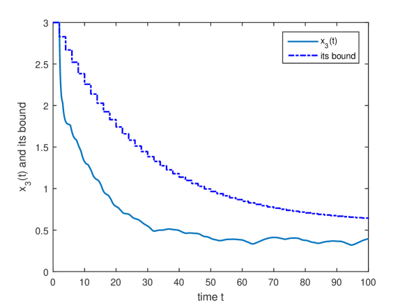
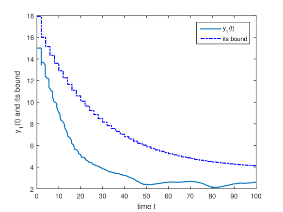
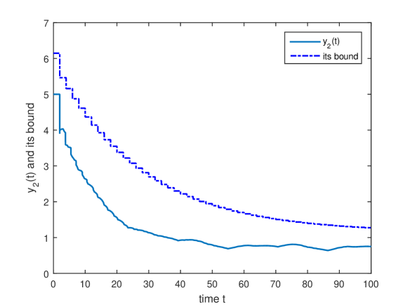
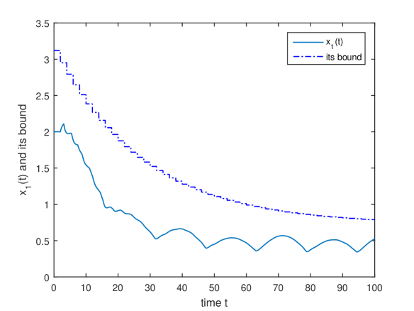
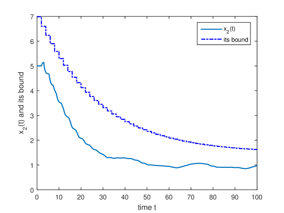
where $a\in\{0,\ 0.5,\ 1\}$; $b\in\{0,\ 1\}$, two time-varying delays as $h_{1}(t)=1+|\sin(t)|$, $h_{2}(t)=1+|\cos(t)|$, and initial values $\psi=\overline{\psi}$, $\phi=\overline{\phi}$. The following figures shows that the trajectories of the partial state vectors of system (1) are bounded by upper bounds computed by Theorem 3.

Figure 1: Trajectories of $x_{1}(t)$ and its bound.

Figure 2: Trajectories of $x_{2}(t)$ and its bound.

Figure 3: Trajectories of $x_{3}(t)$ and its bound.

Figure 4: Trajectories of $y_{1}(t)$ and its bound.

Figure 5: Trajectories of $y_{2}(t)$ and its bound.

5 Conclusion

This paper has studied the problem of finding state bounds for a class of positive CDDEs perturbed by unknown-but-bounded disturbances. A novel method to derive componentwise state bounds on infinite time horizon, the smallest ultimate bound and the smallest invariant set for the system has been presented. A numerical example is considered to illustrate the obtained result.

6 Acknowledgments

This work was supported by the Vietnam Institute for Advantaged Study Mathematics and the National Foundation for Science and Technology Development, Vietnam under the grant 101.01-2017.300.

References

• 1. Niculescu, S.-I.: ’Delay effects on stability: A robust control approach’ Lecture notes in control and information science, vol 269, (Springer: London, 2001)
• 2. Răsvan, V.: ’Functional differential equations of lossless propagation and almost linear behavior’, IFAC Proc. Vol., 2006, 39, (10), pp. 138-150
• 3. Pepe, P., Jiang, Z.P., Fridman, E.: ’A new Lyapunov-Krasovskii methodology for coupled delay differential and difference equations’, Int. J. Control, 2008, 81, (1), pp. 107-115
• 4. Gu, K., Liu, J.: ’Lyapunov-Krasovskii functional for uniform stability of coupled differential-functional equations’, Automatica, 2009, 45, (3), pp. 798-804
• 5. Gu, K.: ’Stability problem of systems with multiple delay channels’, Automatica, 2010, 46, (4), pp. 743-751
• 6. Li, H., Gu, K.: (2010). ‘Discretized Lyapunov-Krasovskii functional for coupled differential-difference equations with multiple delay channels’, Automatica, 2010, 46, (5), pp. 902-909
• 7. Gu, K., Zhang, Y., Xu, S.: ’Small gain problem in coupled differential-difference equations, time-varying delays, and direct Lyapunov method’, Int. J. Robust Nonlin. Control, 2011, 21, (4), pp. 429-451
• 8. Shen, J., Zheng, W.X.: ’Positivity and stability of coupled differential-difference equations with time-varying delays’, Automatica, 2015, 57, pp. 123-127
• 9. Ngoc, P.H.A.: ’Exponential stability of coupled linear delay time-varying differential difference equations’, IEEE Trans. Autom. Control, 2018, 63, (3), pp. 643-648
• 10. Pathirana, P.N., Nam, P.T., Trinh, H.: ’Stability of positive coupled differential-difference equations with unbounded time-varying delays’, Automatica, 2018, 92, pp. 259-263
• 11. Cui, Y., Shen, J., Feng, Z., Chen, Y: ’Stability analysis for positive singular systems with time-varying delays’, IEEE Trans. Automat. Control, 2018, 64, (5), pp. 1487-1494
• 12. Cui, Y., Shen, J., Chen, Y: ’Stability analysis for positive singular systems with distributed delays’, Automatica, 2018, 94, pp. 170-177
• 13. Sau, N. H., Niamsup, P., Phat, V. N.: ’Positivity and stability analysis for linear implicit difference delay equations’, Linear Algebra Appl., 2016, 510, pp. 25-41
• 14. Sau, N. H., Phat, V. N., Niamsup, P.: ’On finite-time stability of linear positive differential-algebraic delay equations’, IEEE Trans. Circuits Syst II Express Briefs, 2018,(Early Access)
• 15. Boyd, S., Ghaoui, L.El., Feron, E., Balakrishnan, V.: ’Linear matrix inequalities in system and control theory’ (Stud. Appl. Numer. Math. 15, SIAM, Philadelphia, 1994)
• 16. Khalil, H.: Nonlinear systems (New Jersey: Prentice-Hall, 3nd edn. 2002)
• 17. Fridman, E., Shaked, U.: ’On reachable sets for linear systems with delay and bounded peak inputs’, Automatica, 39 (2003), pp. 2005-2010
• 18. Kwon, O.M., Lee, S.M., Park, J.H.: ‘On the reachable set bounding of uncertain dynamic systems with time-varying delays and disturbances’, Inf. Sci., 2011, 181, (17), pp. 3735-3748
• 19. Feng, Z., Lam, J.: ’On reachable set estimation of singular systems’, Automatica, 2015, 52, pp. 146-153
• 20. Lam, J., Zhang, B., Chen, Y., Xu, S.: ’Reachable set estimation for discrete-time linear systems with time delays’, Int. J. Robust Nonlin. Control, 2015, 25, (2), pp. 269-281
• 21. Nam, P.T., Pathirana, P.N., Trinh, H.: ’Convergence within a polyhedron: controller design for time-delay systems with bounded disturbances’, IET Control Theory Appl., 2015, 6, (9), pp. 905-914
• 22. Thuan, M.V., Trinh, H., Huong D.C.: ’Reachable sets bounding for switched systems with time-varying delay and bounded disturbances’ Int. J. Systems Sci., 2017, 48, (03), pp. 494-504
• 23. Li, J., Feng, Z., Zhang, C.: ’Reachable set estimation for discrete-time singular systems’, Asian J. Control, 2017, 19, (5), pp. 1862-1870
• 24. Liu, G., Xu, S., Wei, Y., Qi, Z., Zhang, Z.: ’New insight into reachable set estimation for uncertain singular time-delay systems’ Appl. Math. Comput., 2018, 320, pp. 769-780
• 25. Trinh, H., Nam, P.T., Pathirana,P.N., Le, H.P.: ’On backwards and forwards reachable sets bounding for perturbed time-delay systems’, Appl. Math. Computat., 2015, 269, pp. 664-673
• 26. Trinh, H., Hien, L.V.: ’On reachable set estimation of two-dimensional systems described by the Roesser model with time-varying delays’ Int. J. Robust Nonlin. Control, 2018, 28, (1), pp. 227-246
• 27. Kofman E., Haimovich H., Seron M.M.: ’A systematic method to obtain ultimate bounds for perturbed systems’, Int. J. Control, 2007, 80, (2), pp. 167-178.
• 28. Haimovich, H., Seron, M.M.: ’Bounds and invariant sets for a class of switching systems with delayed-state-dependent perturbations’, Automatica, 2013, 49, (3), pp. 748-754
• 29. Du, B., Lam, J., Shu, Z., Chen, Y.: ’On reachable sets for positive linear systems under constrained exogenous inputs’ Automatica, 2016, 74, pp. 230-237
• 30. Nam, P.T., Pathirana, P.N., Trinh, H.: ’Reachable set bounding for nonlinear perturbed time-delay systems: The smallest bound’, Appl. Math. Lett., 2015, 43, (9), pp. 68-71
• 31. Nam, P.T., Pathirana, P.N., Trinh, H.: ’Partial state bounding with a pre-specified time of non-linear discrete systems with time-varying delays’, IET Control Theory Appl., 2016, 10 (13), pp. 1496 1502
• 32. Nam, P. T., Trinh, H., Pathirana P. N.: ’Componentwise ultimate bounds for positive discrete time-delay systems perturbed by interval disturbances’, Automatica, 2016, 72, pp. 153-157
• 33. Kaczorek, T.: ’Positive 1D and 2D systems’ (Springer-Verlag, London, 2002)
• 34. Berman, A., Plemmons, R.J.: ’Nonnegative matrices in the mathematical science’ (Academic Press, New York, 1979)
• 35. Ngoc, P.H.A., Trinh, H.: ’Novel criteria for exponential stability of linear neutral time-varying differential systems’, IEEE Trans. Autom. Control, 2016, 61, (6), pp. 1590-1594