Large Deviations of Convex Hulls of the “True” Self-Avoiding Random Walk

Abstract

We study the distribution of the area and perimeter of the convex hull of the “true” self-avoiding random walk in a plane. Using a Markov chain Monte Carlo sampling method, we obtain the distributions also in their far tails, down to probabilities like $10^{-800}$. This enables us to test previous conjectures regarding the scaling of the distribution and the large-deviation rate function $\Phi$. In previous studies e.g., for standard random walks, the whole distribution was governed by the Flory exponent $\nu$. We confirm this in the present study by considering expected logarithmic corrections. On the other hand, the behavior of the rate function deviates from the expected form. For this exception we give a qualitative reasoning.

1 Introduction

The random walk is a very simple model for diffusive processes with Brownian motion [1] as the prime example. Though its applications range from financial models [2] over online search engines [3] to the very sampling algorithm used in this study [4]. Its simplest variation lives on a lattice and takes steps on random adjacent sites at each timestep, which is exceptionally well researched [5]. With the further constraint that no site may be visited twice, such that the walk is self-avoiding, it becomes a simple model for polymers [6]. Interestingly, depending on the exact protocol how the self-avoidance is achieved, they can also be used to study the perimeter of, e.g., critical percolation clusters [7] or spanning trees [8, 9]

The distance of a random walk from its starting point is the most prominent and simple measurable quantity. Nevertheless, here we go beyond this by considering the convex hull of all $T$ sites visited by the random walk, i.e., the smallest convex polygon containing all these sites. It can be seen as a measure of the general shape of the random walk, without exposing all details of the walk. Thus, the area $A$ or perimeter $L$ of the convex hull can then be used to characterize the random walk in a very simple way. This method is also used, for example, to describe the home ranges of animals [10, 11, 12], spread of animal epidemics [13] or classification of different phases using the trajectory of intermittent stochastic processes [14]. For standard random walks its mean perimeter [15] and mean area [16] in the large $T$ limit are known exactly since a long time. More recently different approaches generalized these results to multiple random walks [17, 18] and arbitrary dimensions [19]. Even more recently the mean perimeter and area for finite (but large) walk lengths $T$ were computed explicitly [20] if the random walk is discrete-time with jumps from an arbitrary distribution. If the distribution of the jump length is Gaussian, even an exact combinatorial formula for the mean volume in arbitrary dimensions is known [21]. For higher moments however, there is only one analytic result for the special case of Brownian bridges [22], i.e., closed walks with Gaussian jumps. When asking for more, i.e., for the full distributions, no exact analytical results are available. This motivated the numerical study of the full distributions—or at least large parts of the support—using large-deviation sampling techniques to sample even far into the tails of standard random walks [23] and multiple random walks [24], also in higher dimensions [25]. These numerical studies are rather expensive, since they usually require Markov chain Monte Carlo simulations, allowing one to measure the distribution in regions where the probabilities are as small as $10^{-100}$.

Since self-avoiding walks are considerably more difficult to treat analytically than standard random walks, there are no analytical results about the properties of their convex hulls yet. Therefore, the authors of this contribution very recently published a numerical study of the full distribution of perimeter and area of three different types of self-avoiding random walks [26], notably the classical self-avoiding walk (SAW) and the smart kinetic self-avoiding walk (SKSAW). While the SAW is combinatorial in nature and describes the set of all self-avoiding configurations with equal probability, the SKSAW is a growth process, which assigns more weight to some configurations. In [26] we also give an estimate for the functional form of the rate function $\Phi$ describing the far right tail behavior of the distribution, i.e., $P(S)\approx\operatorname{e}^{-T\Phi(S)}$. It was found to depend only on the dimension $d$ and the scaling exponent $\nu$. For two-dimensional random walks these scaling exponents are often known exactly through Schramm-Loewner evolution [27, 28, 29, 30].

In this study we test this prediction for the “true” self-avoiding walk (TSAW), which has a free parameter $\beta$ governing how strictly self-avoiding the walk is. Introduced in [31] the TSAW was a counter model to the SAW, especially it should demonstrate that the behavior of the combinatorial SAW is very different from more natural growing random walks which avoid themselves. Indeed, in two dimensions, where the end-to-end distance $r$ of a $T$ step SAW scales as $r\propto T^{\nu}$ with $\nu=3/4$, the TSAW will scale as

$$r\propto T^{\nu}\left(\ln T\right)^{\alpha}$$ (1)

with $\nu=1/2$ [32] and a correction $\alpha$, which is not known rigorously, but estimated as $\alpha=1/4$ [33]. Here we show, for large-enough values of $\beta$, that in contrast to previous work [26] the rate function $\Phi$ is not simply determined by the value of $\nu$, since the growth process of the TSAW in the large-area region of the tail is indistinguishable from the SKSAW growth process, although they have different values of the scaling exponent $\nu$ determined by the behavior of the high-probability part of their distributions.

2 Models and Methods

This section will introduce the TSAW model and the sampling method in enough detail to reproduce the results of this study. For more fundamental methods, like the construction of the convex hull, we will sketch the main ideas.

2.1 Large Deviation Sampling Scheme

To obtain good statistic in the far tail, it is not sufficient to perform naive simple sampling, since configurations of probability $P$ would need about $1/P$ samples to occur at all. It is therefore not feasible to explore the distributions down to the tails of $P<10^{-100}$ with simple sampling. Instead we use an importance sampling scheme to generate more samples in the low probability tails. Thus, we generate Markov chains consisting of sequences of TSAWs and use the well known Metropolis algorithm [34] with a Boltzmann sampling weight. For this purpose, we identify the quantity $S$ we are interested in—here the area $A$ but it could be any measurable quantity in principle—with the energy occurring in the Boltzmann factor and introduce an artificial “temperature” $\Theta$. Since the TSAW is a growth process, it is not trivial to come up with a local change move within the Markov chain, i.e., it is difficult to change a configuration by a small amount while preserving the correct statistics. Therefore our Markov chain is not directly a chain of configurations of TSAW but rather a chain of random number vectors $\bm{\xi}_{i}$. Each vector $\bm{\xi}_{i}$ determines a configuration of a TSAW by performing the growth process and using for each of the $T$ decisions a random number from $\bm{\xi}_{i}$. This approach is sketched in Fig. 1 and extremely general since it can be applied to any model [35]. A change move is a simple change of one entry of $\bm{\xi}_{i}$.

Figure 1: Sketch of the Markov chain of random number vectors $\bm{\xi}_{i}$. The change move is performed on the $\bm{\xi}_{i}$ and a new TSAW is generated from scratch, its energy difference to the previous configuration is used to accept or reject the change.

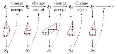
Following the Metropolis algorithm, we propose a new $\bm{\xi}^{\prime}$ by replacing a random entry with a new random number $\xi\in U[0,1)$, generate a new TSAW configuration from scratch using the random numbers $\bm{\xi}^{\prime}$ and calculating its energy $S^{\prime}$, i.e., its area. The proposed configuration is then accepted, i.e., $\bm{\xi}_{i+1}=\bm{\xi}^{\prime}$, or rejected, i.e., $\bm{\xi}_{i+1}=\bm{\xi}_{i}$, depending on the temperature and energy difference with respect to the previous configuration with probability $p_{\mathrm{acc}}=\operatorname{e}^{-\Delta S/\Theta}$, where $\Delta S=S^{\prime}-S_{i}$ is the energy difference caused by the change. Replacing a random entry by a new entry is clearly ergodic, since any possible $\bm{\xi}_{i}$ can be generated this way. Since we use the classical Metropolis acceptance probability, detailed balance is also given. This Markov process will therefore yield configurations $\bm{\xi}$ according to their equilibrium distribution $Q_{\Theta}(\bm{\xi})=\frac{1}{Z(\Theta)}Q(\bm{\xi})\operatorname{e}^{-S(\bm{\xi})/\Theta},$ where $Q(\bm{\xi})$ is the natural, unbiased distribution of configurations and $Z(\Theta)$ the corresponding partition function. For small temperatures this will lead to small energies, i.e., smaller than typical perimeters or areas. For large temperatures typical configurations will be generated and for negative temperatures larger than usual energies dominate. Since this Metropolis algorithm will generate instances following a Boltzmann distribution we can easily undo this bias, i.e., we can derive the actual distribution $P(S)$ from the biased, temperature dependent distributions $P_{\Theta}(S)$ as

$$P_{\Theta}(S) =\sum_{\{\bm{\xi}|S(\bm{\xi})=S\}}Q_{\Theta}(\bm{\xi})$$ (2)

$$=\sum_{\{\bm{\xi}|S(\bm{\xi})=S\}}\frac{\exp(-S/\Theta)}{Z(\Theta)}Q(\bm{\xi})$$ (3)

$$=\frac{\exp(-S/\Theta)}{Z(\Theta)}P(S).$$ (4)

The unknown $Z(\Theta)$ can be numerically determined by enforcing the continuity of the distribution. Therefore we need to simulate the system at many different temperatures $\Theta$, such that all histograms $P_{\Theta}(S)$ overlap with adjacent temperatures. $Z(\Theta)$ can now be calculated in overlapping regions, which should coincide for continuity, i.e.,

$$\operatorname{e}^{S/\Theta_{i}}Z(\Theta_{i})P_{\Theta_{i}}(S) =\operatorname{e}^{S/\Theta_{i+1}}Z(\Theta_{i+1})P_{\Theta_{i+1}}(S)$$ (5)

$$\Rightarrow\quad\frac{Z(\Theta_{i})}{Z(\Theta_{i+1})} =\exp\left({S/\Theta_{i+1}-S/\Theta_{i}}\right)\frac{P_{\Theta_{i+1}}(S)}{P_{\Theta_{i}}(S)}.$$ (6)

This relation fixes all ratios of consecutive $Z(\Theta)$. The absolute value can be fixed by the normalization of the whole distribution.

This method is applicable to a wide range of models, and already successfully applied to obtain, e.g., the distributions over a large range for the score of sequence alignments [36, 37, 38], work distributions for non-equilibrium systems [35], properties of Erdős Rényi random graphs [39, 40, 41], and in particular to obtain statistics of the convex hulls of a wide range of types of random walks [23, 24, 26].

2.2 “True” Self-Avoiding Walk

The “true” self-avoiding Walk (TSAW) is a random walk model, in which the walker tries to avoid itself, but self-avoidance is not strictly imposed.

(a) $\beta=0$

(b) $\beta=1$

(c) $\beta=100$

Figure 2: Examples of typical TSAW realizations at different values of the avoidance parameter $\beta$ with their convex hulls. Each walk has $T=200$ steps. Larger values of $\beta$ lead to larger extended walks characterized by larger areas of their convex hulls.

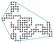
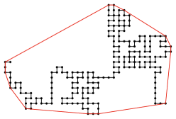
To construct a TSAW realization one grows a standard random walk on a lattice and records the number of visits $n_{i}$ to each site $i$. For each step the probability to step on a neighboring site $i$ is weighted with the number of times that site was already visited

$$p_{i}=\frac{\exp\left(-\beta n_{i}\right)}{\sum_{j\in\mathcal{N}}\exp\left(-\beta n_{j}\right)},$$ (7)

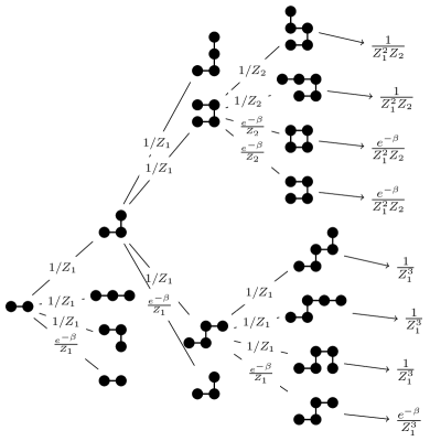
where the sum over all current neighbors $\mathcal{N}$ is for normalization. The free parameter $\beta$ governs the strength of the avoidance. Large values of $\beta$ lead to stronger avoidance, negative values of $\beta$ lead to attraction and $\beta=0$ is the special case of the standard random walk. For a selection of $\beta$ values typical examples are visualized in Fig. 2. The TSAW is not to be confused with the classical self-avoiding walk (SAW), which describes the ensemble of all configurations which do not intersect themselves each weighted the same. In Fig. 3 two partial decision trees are displayed which visualize the fundamental differences in the weights of the configurations. Even in the $\beta\to\infty$ limit ($Z_{1}=3$, $Z_{2}=2$) the weights differ. In particular its upper critical dimension is $d=2$ [31], which means that the exponent $\nu$, which characterizes the scaling of the end-to-end distance $r\propto T^{\nu}$, is $\nu=1/2$ with logarithmic corrections, i.e., $r\propto T^{\nu}\left(\ln T\right)^{\alpha}$, where $\alpha=1/4$ [33] is conjectured.

(a) SAW

(b) TSAW

Figure 3: Partial decision trees for SAW and TSAW of walks up to length $T=5$. On the right side of each tree the weight of the configuration is displayed. While the weights for the SAW are by definition uniform for every valid configuration, the TSAW not only allows self-intersection, but also has different weights depending on the history of the walk. Note that $Z_{1}=3+\exp(-\beta)$ and $Z_{2}=2+2\exp(-\beta)$.

2.3 Convex Hulls

The convex hull of a set of points $\mathcal{P}$ in the plane is the smallest convex polygon enclosing every point $p\in\mathcal{P}$ and hence also every line between any pair of points. Some examples of convex hulls are visualized in Fig. 2. The construction of a convex hull of a planar point set is a solved problem, in the sense that an optimal algorithm exists [42, 43] with result-dependent run time $\mathcal{O}(T\log h)$, where $T$ is the number of points $|\mathcal{P}|$ and $h$ is the number of vertices of the resulting convex hull. In practice, however, suboptimal but simpler and for point sets as small as in this study ($T\approx 10^{6}$) faster algorithms are used. Especially for planar point sets one can exploit the fact that a polygon can be defined by the order of its vertices, instead by a list of its facets. The Graham scan [44] algorithm is based on this fact. After shifting the coordinate origin into the center of the point set, it sorts the points according to their polar coordinate. Then starting at an arbitrary point all points are filtered out which are oriented clockwise with respect to the the previous and next (not-filtered out) points. Iterating this over a full revolution, leaves only the points which constitute the vertices of the convex hull. This algorithm is dominated by the time to sort the points, which can be done in $\mathcal{O}(T\log T)$. Here, we use Andrew’s monotone chain algorithm [45], which is a variation of the Graham scan sorting the points lexicographically, which is slightly faster, instead of by polar angle. Note that this type of algorithm does not generalize to $3$ or higher dimensions. For those cases a different algorithm, like quickhull [46] has to be used. Before applying the exact algorithm, we reduce the size of the point set with Akl’s elimination heuristic [47], which removes all points inside, in our implementation, a octagon of extreme points. Of a few tested polygons the octagon showed the best performance in the instances we typically encounter in this study.

To calculate the area $A$ of a convex polygon, where the coordinates are sorted counterclockwise, one can sum the areas of the trapezoids extending perpendicular to the $x$-axis

$$A =\frac{1}{2}\sum_{i=0}^{h-1}(y_{i}+y_{i+1})(x_{i}-x_{i+1}).$$ (8)

The perimeter $L$ is the sum of the line segments of consecutive points of the hull

$$L =\sum_{i=0}^{h-1}\sqrt{(x_{i}-x_{i+1})^{2}+(y_{i}+y_{i+1})^{2}},$$ (9)

with $x_{h}\equiv x_{0}$ and $y_{h}\equiv y_{0}$.

3 Results

We simulated the TSAW at two values of $\beta$. The limit case of a TSAW, which only steps on itself, if it has no other choice, was simulated at $\beta=100$. Since the probability to step on already visited sites is exponential in $\beta$, this corresponds to the $\beta\to\infty$ case. Further, we simulated at $\beta=1$, to capture also the case, which does sometimes voluntarily step on itself.

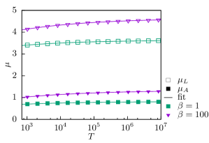
First, we will look at the behavior of the mean of the perimeter and area. Here, we used simple sampling for walk lengths in the range $T\in\{2^{k}|10\leq k\leq 23\}$. Each value is averaged over $10^{6}$ TSAWs. Naturally, the mean of geometric volumes scale with their intrinsic dimension $d_{i}$ and a typical length scale $r$, e.g., the end-to-end distance, as $r^{d_{i}}$. Using the scaling of $r$ from Eq. (1), we expect the mean values of the perimeter $\left<L\right>$ ($d_{i}=1$ in $d=2$) and the area $\left<A\right>$ ($d_{i}=2$) to scale as

$$S\propto T^{d_{i}\nu}\ln(T)^{d_{i}\alpha}$$ (10)

for large values of $T$. We can even calculate the asymptotic prefactors $\mu^{\infty}$ by extrapolating the scaled values for finite sizes $\mu_{L}=\left<L\right>T^{-1/2}\ln(T)^{-\alpha}$ and $\mu_{A}=\left<A\right>T^{-1}\ln(T)^{-2\alpha}$ to their asymptotic values $\mu_{L}^{\infty}$ and $\mu_{A}^{\infty}$. For the extrapolation, which is shown in Fig. 4(a), we use a simple power law with offset $\mu=\mu^{\infty}-aT^{-b}$, which were already used for this purpose in [23, 24]. The asymptotic values are listed in table 1. As expected the values for the TSAW are larger for larger $\beta$. To our knowledge, there are no analytical calculations for these asymptotic values to which we could compare to. The given error estimates are only statistical and do not include the systematic error introduced by the ad-hoc fit function. Nevertheless the convergence of the values is very well visible, confirming $\nu=1/2$ and $\alpha=1/4$ to be very good estimates.

Direct fits of the form Eq. (10) yield values in good agreement with the expected exponents for the end-to-end distance $r$ at $\beta=1$, but most other data sets lead to fits overestimating $\alpha$ and slightly underestimating $\nu$. A possible, at least partial, explanation for this is be that the relation $L(r)$ is not perfectly linear for the sizes we obtained data for.

(a) Asymptotic mean values

(b) Comparison of different types of random walks

Figure 4: 4(a) Extrapolation of the asymptotic mean values of the perimeter and area of the convex hull. 4(b) Distribution of all scrutinized walk types with $T=1024$ steps. The inset shows the peak region. Note that the standard random walk (RW) and the $\beta=0$ TSAW coincide. Also the far right tail of the $\beta=100$ TSAW and SKSAW coincide, but not the main region. The vertical line shows the maximum area constructable with $1024$ steps, which has an area $A_{\max}$ about $512^{2}/2\approx 1.3\times 10^{5}$. The distributions are thus not sampled over their whole support, but a large region.

	$\mu_{L}^{\infty}$	$\mu_{A}^{\infty}$
TSAW $\beta=0$ (exact)	$3.5449...$	$0.7854...$
TSAW $\beta=1$	$3.636(2)$	$0.820(1)$
TSAW $\beta=100$	$4.641(3)$	$1.339(3)$

Table 1: Asymptotic mean values of the area and perimeter scaled by Eq. (10). The values are obtained by the fit shown in Fig. 4(a). The given error estimates are only statistical and do not include the systematic error introduced by the ad-hoc fit function. The exact values are from [19] and converted to a square lattice as described in [26].

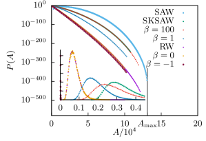
We now focus on the main result, on the distribution $P(A)$ of the convex-hull area. These results were obtained using the large-deviation Markov-chain simulations. We had to perform simulations for different “temperatures” ranges for each system size and parameter $\beta$. For example $T=128$ at $\beta=1$ needed seven temperatures for the right tail $\theta\in[-40,-9]$ and three more for the left $\theta\in[7,40]$. For larger system sizes more temperatures are usually needed. For the $\beta=1$ case at $T=2048$ we used 32 temperatures $\theta\in[-3200,-105]$ to obtain the right tail. For the $\beta=100$ cases we could use similar values for the temperatures. Equilibration was ensured as described in [26]. In Figure 4(b) we compare distributions of different random walk types with the result for the TSAW at different values of $\beta$. By using the large-deviation algorithm, we were able to obtain this distribution over hundreds of decades in probability, down to values as small as $P(A)\sim 10^{-800}$ for the largest value of $T$. Notice that while SKSAW and TSAW with high values of $\beta$ show the same behavior in the far tail, where the walks are so stretched out such that trapping does not play a role anymore. In the main region however, they are clearly distinct, as is expected due to their different scaling exponent $\nu$. Further, the parameter $\beta$ can apparently be used to interpolate the tail behavior between the standard random walk case and the SKSAW case.

Since we have obtained large parts of the distribution, it would be interesting if the whole distribution scales the same as the mean values (cf. Eq. (10)). For other types of walks, the distribution of perimeter and area could indeed be scaled [23, 24, 25, 26] across their full support only knowing $\nu$, as

$$P(S)=T^{-d\nu}\widetilde{P}\left(ST^{-d\nu}\right).$$ (11)

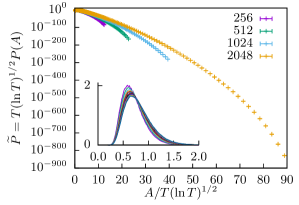
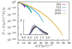
For the TSAW, this collapse, when considering the logarithmic corrections as visualized in Fig. 5, exhibits an apparent drift towards a limiting shape. Nevertheless, severe finite size effects are visible, especially in the tails but also in the main region. Despite far larger system sizes $T$ considered, here the main region collapse is worse than for other kinds of self-avoiding walks as shown in [26]. The stronger finite size effect may be caused by the fact that all walks start on an empty lattice. This means for our case that the first steps of the walk behave differently from the last steps of the walk, when many sites are occupied. Although for the limit of large system sizes $T$, the latter should determine the behavior. A possible improvement to simulate TSAWs is suggested in [33], which is to simulate a much longer walk with $t\gg T$ steps and look at the last $T$ steps.

(a) $\beta=1$

(b) $\beta=100$

Figure 5: Distributions of the area of the “true” self-avoiding random walk scaled according to Eq. (11) plus logarithmic corrections for different values of $\beta$ and lengths $T$. The insets show the main region for 14 values of $T\in\{2^{k}|10\leq k\leq 23\}$ obtained by simple sampling.

The rate function $\Phi$ is defined if the distribution obeys the large deviation principle. This means that the distribution, for large values of $T$, should decay exponentially in the length $T$ scaled by the rate function as

$$P_{T}(s)\approx\operatorname{e}^{-T\Phi(s)}.$$ (12)

Usually the parameter $s$ is between $0$ and $1$. We achieve this by dividing our measured area by the maximum area, i.e., by measuring $s=\frac{A}{A_{\mathrm{max}}}$. In two dimensions the walk configuration with maximum area is L-shaped with arms of equal length (for odd $T$) and therefore $A_{\mathrm{max}}=\frac{1}{2}\left(\frac{T+1}{2}\right)^{2}\approx\frac{T^{2}}{8}$.

Similar to [26] we assume the rate function to be a power law

$$\Phi(s)\propto s^{\kappa},$$ (13)

which seems to agree reasonably well with our data, since the double logarithmic plot Fig. 6 shows that the rate function appears as a straight line in the intermediate tail. The far tail is dominated by finite-size effects caused by the lattice structure, which leads to a “bending up” of the rate function. For small values of $s$, in the high-probability region, the rate function does not have any relevance. Assuming that the rate function is a power law Eq. (13) and scaling of the form Eq. (11) is possible, with $d_{i}$ being the intrinsic dimension of the observable, e.g., $d_{i}=2$ for the area, we can derive a value for the power law exponent of the rate function $\kappa$. Using the definition of the rate function Eq. (12)

$$\operatorname{e}^{-T\Phi(ST^{-d_{i}})}\approx T^{-d_{i}\nu}\widetilde{P}\left(ST^{-d_{i}\nu}\right)$$ (14)

should hold in the right tail. The $T^{-d_{i}\nu}$ term can be ignored next to the exponential, also the logarithmic correction is subdominant and would not allow to add any insight. Apparently the right hand side is a function of $ST^{-d_{i}\nu}$, such that the left hand side also has to be a function of $ST^{-d_{i}\nu}$. This is the case for [26]

$$\kappa=\frac{1}{d_{i}(1-\nu)}.$$ (15)

(a)

(b)

Figure 6: Rate function $\Phi$ for the area with fits to the assumed power-law form. The fit is performed over a range, where the finite-size influence of the lattice should be small, but the large $T$ behavior can be extrapolated. Finite-size effects seem more pronounced for larger values of $\beta$.

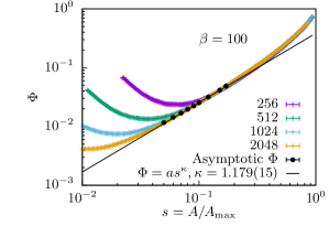
To test whether the results for the rate function in case of the TSAW obeys this relation, we estimate the value of $\kappa$ from our data. Since we have data for various values of the walk length $T$, we first extrapolate our data point-wise to large $T$. For this purpose we fit a power law with offset, where the parameters depend on the value of $s$:

$$\Phi(s,T)=a(s)T^{b(s)}+\Phi_{\infty}(s).$$ (16)

This results in the value of interest $\Phi(s)\equiv\Phi_{\infty}(s)$, the parameters $a(s)$ and $b(s)$ are only auxiliary quantities. We perform this extrapolation in a region which is far away from the finite-size effects of the far tail. In this range of medium values of $s$ the extrapolation according to Eq. (16) works robustly. Since the bins of the logarithmic histograms we use do not have the same borders for every system size $T$, we have a-priory not access to the same value of $s$ for different values of $T$. Thus, we use cubic splines to interpolate such that we obtain results for the same value of $s$ for all walk lengths. We found cubic splines to be sufficient since the bins are rather dense such that systematic errors introduced by the interpolation should be small. The final values $\Phi(s)$ obtained from the extrapolated values to the assumed form Eq. (13) are shown in Fig. 6 as symbols. Next, we fit power laws to this data. The values for $\kappa$ obtained are within errorbars consistent with $\kappa=7/6$ which is the expected value for the SKSAW ($\nu=4/7$) and incompatible with the expected value $\kappa=1$ of $\nu=1/2$ walks. This behavior is nevertheless plausible since in the tail (large-area) region, structures, which enable self trapping, i.e., loops, are rare since they do lead to smaller areas of the convex hull than straight regions. Therefore the influence of trappings should diminish in the large area tail, which is the main difference in the behavior of SKSAW and TSAW. Without trappings the TSAW in the $\beta\to\infty$ limit is functionally identical to the SKSAW. Apparently already $\beta=1$ is large enough to produce this behavior. Therefore it is natural that the large-area tail behaves the same as the SKSAW. On the other hand, to possibly see a range where the rate function behaves like a power law with $\kappa=1$ according to $\nu=1/2$, one would have to go to much larger system sizes, because one would have to obtain data to the right of the peak, but for very small values of $s=A/A_{\max}\ll 10^{-2}$, where trappings still do play a role. In particular the analysis might be hampered by the presence of the logarithmic correction to the mean end-to-end distance.

This means that the TSAW is more complex in comparison to some other types of self-avoiding walks for which it was possible to predict the tail behavior from the same exponent $\nu$ which predicts the mean behavior. The other types of random walk were under scrutiny in [26], namely the self-avoiding walk, the loop-erased random walk and the smart kinetic self-avoiding walk (SKSAW). Instead for TSAW in the large deviation region a different scaling exponent seems to hold, which is very close to the scaling exponent of the SKSAW.

4 Conclusions

We studied the behavior of the distribution of the area of the convex hull of the “true” self-avoiding walk, especially in the large deviation regime of larger than typical areas. With a sophisticated large-deviation sampling algorithm, we obtained the distribution over a large part of its support down to probabilities smaller than $10^{-800}$ for a typical avoidance parameter of $\beta=1$ and a large avoidance $\beta=100$. The distributions seem to approach a limiting scaling form when rescaled by the behavior of the mean, but with much stronger finite-size effects as compared to other types of random walks, which were previously studied.

Using this data we calculated the rate functions. The rate function seem also to behave qualitatively similar in comparison to other types of self-avoiding walks studied earlier [26] in that they seem to be well defined and well approximated by a power law. In contrast to other types of random walks, this power law can apparently not be derived from the scaling exponent of the mean values $\nu$. Instead it seems that a second exponent governs the scaling behavior of the tail for the TSAW, which is close to $4/7$, the scaling exponent of the smart kinetic self-avoiding walk. This is plausible since the large-area region should be dominated by configurations in which no trappings are possible, which is the major difference between these types.

Finally, we also provided estimates for the relevant scale factors of the mean of area and perimeter of the convex hulls of TSAWs. They might be accessible to analytic calculations in the future.

For future numerical work it would be interesting to look for further types of random walks, which show similar effects of distinct scaling exponents for different parts of the distribution but do not show the strong logarithmic corrections to scaling, and would therefore be easier to analyze. On the other hand, it would be very exciting if one was able to obtain data in the range where the rate function exhibits the exponent $\kappa(\nu=1/2)=1$, with the need to simulate really large system sizes, but closer to the typical behavior.

This work was supported by the German Science Foundation (DFG) through the grant HA 3169/8-1. We also thank the GWDG (Göttingen) for providing computational resources.

References

- [1] Einstein A 1906 Annalen der Physik 324 371–381 ISSN 1521-3889
- [2] Fama E F 1965 Financial Analysts Journal 21 55–59
- [3] Page L, Brin S, Motwani R and Winograd T 1999 The pagerank citation ranking: Bringing order to the web. Technical Report 1999-66 Stanford InfoLab
- [4] Newman M and Barkema G 1999 Monte Carlo Methods in Statistical Physics (Clarendon Press) ISBN 9780198517979
- [5] Hughes B D 1996 Random walks and random environments (Clarendon Press Oxford)
- [6] Madras N and Slade G 2013 The Self-Avoiding Walk (New York, NY: Springer New York) ISBN 978-1-4614-6025-1
- [7] Weinrib A and Trugman S A 1985 Phys. Rev. B 31(5) 2993–2997
- [8] Manna S S, Dhar D and Majumdar S N 1992 Phys. Rev. A 46(8) R4471–R4474
- [9] Majumdar S N 1992 Phys. Rev. Lett. 68(15) 2329–2331
- [10] Mohr C O 1947 American Midland Naturalist 37 pp. 223–249
- [11] Worton B J 1987 Ecol. Model. 38 277–298 ISSN 0304-3800
- [12] Boyle S A, Lourenco W C, da Silva L R and Smith A T 2009 Folia Primatol. 80 33–42
- [13] Dumonteil E, Majumdar S N, Rosso A and Zoia A 2013 Proceedings of the National Academy of Sciences 110 4239–4244
- [14] Lanoiselée Y and Grebenkov D S 2017 Phys. Rev. E 96(2) 022144
- [15] Letac G and Takács L 1980 The American Mathematical Monthly 87 142–142 ISSN 00029890, 19300972
- [16] Letac G 1993 Journal of Theoretical Probability 6 385–387 ISSN 1572-9230
- [17] Randon-Furling J, Majumdar S N and Comtet A 2009 Phys. Rev. Lett. 103(14) 140602
- [18] Majumdar S N, Comtet A and Randon-Furling J 2010 Journal of Statistical Physics 138 955–1009 ISSN 1572-9613
- [19] Eldan R 2014 Electron. J. Probab. 19 no. 45, 1–34 ISSN 1083-6489
- [20] Grebenkov D S, Lanoiselée Y and Majumdar S N 2017 Journal of Statistical Mechanics: Theory and Experiment 2017 103203
- [21] Kabluchko Z and Zaporozhets D 2016 Transactions of the American Mathematical Society 368 8873–8899
- [22] Goldman A 1996 Probability Theory and Related Fields 105 57–83 ISSN 1432-2064
- [23] Claussen G, Hartmann A K and Majumdar S N 2015 Phys. Rev. E 91(5) 052104
- [24] Dewenter T, Claussen G, Hartmann A K and Majumdar S N 2016 Phys. Rev. E 94(5) 052120
- [25] Schawe H, Hartmann A K and Majumdar S N 2017 Phys. Rev. E 96(6) 062101
- [26] Schawe H, Hartmann A K and Majumdar S N 2018 Phys. Rev. E 97(6) 062159
- [27] Cardy J 2005 Annals of Physics 318 81 – 118 ISSN 0003-4916 special Issue
- [28] Lawler G F, Schramm O and Werner W 2002 arXiv preprint math/0204277
- [29] Lawler G F, Schramm O and Werner W 2011 Conformal Invariance Of Planar Loop-Erased Random Walks and Uniform Spanning Trees (New York, NY: Springer New York) pp 931–987 ISBN 978-1-4419-9675-6
- [30] Kennedy T 2015 Journal of Statistical Physics 160 302–320 ISSN 1572-9613
- [31] Amit D J, Parisi G and Peliti L 1983 Phys. Rev. B 27(3) 1635–1645
- [32] Pietronero L 1983 Phys. Rev. B 27(9) 5887–5889
- [33] Grassberger P 2017 Phys. Rev. Lett. 119(14) 140601
- [34] Metropolis N, Rosenbluth A W, Rosenbluth M N, Teller A H and Teller E 1953 The Journal of Chemical Physics 21 1087–1092
- [35] Hartmann A K 2014 Phys. Rev. E 89(5) 052103
- [36] Hartmann A K 2002 Phys. Rev. E 65(5) 056102
- [37] Wolfsheimer S, Burghardt B and Hartmann A K 2007 Algorithms for Molecular Biology 2 9 ISSN 1748-7188
- [38] Fieth P and Hartmann A K 2016 Phys. Rev. E 94(2) 022127
- [39] Engel A, Monasson R and Hartmann A K 2004 Journal of Statistical Physics 117 387–426 ISSN 1572-9613
- [40] Hartmann A K 2011 The European Physical Journal B 84 627–634 ISSN 1434-6036
- [41] Hartmann A K and Mézard M 2018 Phys. Rev. E 97(3) 032128
- [42] Kirkpatrick D and Seidel R 1986 SIAM Journal on Computing 15 287–299
- [43] Chan T M 1996 Discrete & Computational Geometry 16 361–368 ISSN 1432-0444
- [44] Graham R 1972 Information Processing Letters 1 132–133
- [45] Andrew A 1979 Information Processing Letters 9 216 – 219 ISSN 0020-0190
- [46] Barber C B, Dobkin D P and Huhdanpaa H 1996 ACM Trans. Math. Softw. 22 469–483 URL http://www.qhull.org
- [47] Akl S G and Toussaint G T 1978 Information Processing Letters 7 219 – 222 ISSN 0020-0190